S. Andova et.al. (Eds.): Workshop on Quantitative Formal Methods: Theory and Applications (QFM’09)
EPTCS 13, 2009, pp. 67–78, doi:10.4204/EPTCS.13.6
c
H. Wang & W. MacCaull This work is licensed under the Creative Commons Attribution License.
Methods
Hao Wang and Wendy MacCaull Centre for Logic and Information
St. Francis Xavier University Antigonish, Canada {hwang, wmaccaul}@stfx.ca
Timed model checking has been extensively researched in recent years. Many new formalisms with time extensions and tools based on them have been presented. On the other hand, Explicit-Time Description Methodsaim to verify real-time systems with general untimed model checkers. Lamport presented an explicit-time description method using a clock-ticking process (Tick) to simulate the passage of time together with a group of global variables for time requirements. This paper proposes a new explicit-time description method with no reliance on global variables. Instead, it uses rendezvous synchronization steps between theTickprocess and each system process to simulate time. This new method achieves bettermodularityand facilitates usage of more complex timing constraints. The two explicit-time description methods are implemented in DIVINE, a well-known distributed-memory model checker. Preliminary experiment results show that our new method, with better modularity, is comparable to Lamport’s method with respect to time and memory efficiency.
1
Introduction
Model checking is an automatic analysis method which explores all possible states of a modeled sys-tem to verify whether the syssys-tem satisfies a formally specified property. It was popularized in industrial applications, e.g., for computer hardware and software, and has great potential for modeling and moni-toring complex and distributed business processes.Timedmodel checking, the method to formally verify real-time systems, is attracting increasing attention from both the model checking community and the real-time community. However, general model checkers like SPIN [14] can only represent and verify thequalitativerelations between events, which constrains their use for real-time systems. Thequantified
time notions, including time instant and duration, must be taken into account for timed model checking. For example in a safety critical application such as in an emergency department, after an emergency case arrives at the hospital, general model checking of hospital protocol can only verify whether “the patient receives a certain treatment”, but to save the patient’s life, it should be verified whether the protocol ensures that “the patient receives a certain treatment within 1 hour”.
a time region; such model checkers can only deal with specification involving a time region or a pre-specified time instant. However, many real-time systems, especially those with pre-emptive scheduling features, need to record the time instant when the pre-emption happens for succeeding calculation. For example, triage is widely practiced in medical procedures; the caregiverC may be administering some required but non-critical treatment on patientAwhen another patientBpresents with a critical situation, such as a cardiac arrest. Cthen must move to the higher priority task of treatingB, but it is necessary to store the elapsed time ofA’s treatment to determine how much time is still needed or the treatment needs to be restarted. Thestop-watchautomata [4], an extension of timed autamata, is proposed to tackle this; unfortunately as Krc´al and Yi discussed in [15], since the reachability problem for this class of automata is undecidable, there is no guarantee for termination in the general case.
On the other hand, Lamport [16] advocated the Explicit-Time Description Methods which aim to use ordinary model checkers to realize timed model checking. He presented an explicit-time description method using a clock-ticking process (Tick) to simulate the passage of time and a pair of global variables to store the time lower and upper bounds for each modeled system process. The main advantage of the explicit-time approach is that it doesnotneed specialized languages or tools for time description. The method has been implemented with popular model checkers SPIN (sequential) [14] and SMV [17]. Re-cently, Van den Berg et al. [10] successfully applied LEDM to verify the safety of railway interlockings for one of Australia’s largest railway companies. The additional benefit of the explicit-time approach is that as it explicitly records the passage of time so the current time instant can be accessed easily, the pre-emptive scheduling problem discussed in the previous paragraph that causes difficulty using the timed-automata-based model checkers can be modeled naturally with explicit-time description methods. In this paper, we propose a new explicit-time description method called Sync-based Explicit-time Description Method(SEDM), which does not rely on global variables; instead it uses rendezvous syn-chronization steps between theTickprocess and each system process. After theTickprocess completes synchronization steps with every system processes, the global clock increments by one time unit. While, as Lamport commented [16], “The approach (LEDM) cannot be used in process-based languages and formalisms with no explicit global state, such as CCS, CSP, Petri nets, streams and I/O automata”, SEDM can do exactly that. As an added advantage, SEDM allows the timing constraints to be defined either globally or locally so the whole system can be modeled in a way that enhances its modularity. We choose DIVINE [7], a well-known distributed model checker, because it accommodates the up-to-date multi-core architecture, i.e., clusters of multi-core CPU’s and it has been tested successfully in large-scale clusters, even in a large-scale optical grid [19]. Experimental results show that SEDM is comparable to LEDM with respect to time and memory efficiency so SEDM can be used in place of LEDM.
The remainder of the paper is organized as follows. After a brief introduction to DIVINE, Section 2 presents the LEDM with its DIVINE implementation. The new method SEDM with its DIVINE implementation is presented in Section 3. Section 4 describes our experiments and the results. Section 5 concludes the paper.
2
Preliminaries
2.1 TheDIVINEModel Checker and its Modeling Language
DIVINE is an explicit-state LTL model checkers based on the automata-based procedure by Vardi and
Wolper [18]. The property to be specified is described by an LTL formula, both the system model and the LTL formula are represented by automata, then the model checking problem is reduced to detecting in the combined automaton graph whether there is anaccepting cycle, i.e., a cycle in which one of the vertices is marked “accepting”. With the distributed algorithms to assign different portions of the state space to be explored by different machines, DIVINE can: (1) verify much larger system models; (2) finish the verification in significantly less time (in comparison with the well-known explicit-state LTL model checker SPIN).
DVE is the modeling language of DIVINE. Like in Promela (the modeling language of SPIN), a model described in DVE consists of processes, message channels and variables. Each process, identified by a unique name procid, consists of a list of local variable declarations, process states declarations, initial state declaration and a list of transitions. A transition transfers the process state fromstateid1to stateid2, the transition may contain a guard (which decides whether the transition can be executed), a
synchronization (which communicates data with another process) and effects (which assigns new values to local or global variables). So we have
Transition ::= stateid1 -> stateid2 { Guard Sync Effect }
TheGuardcontains the keywordguardfollowed by a boolean expression and theEffectcontains the keywordeffectfollowed by a list of assignments. TheSyncfollows the denotation for communi-cation in CSP, ‘!’ for the sender and ‘?’ for the receiver. The synchronization can be either asynchronous or rendezvous. Thechanid is the channel for the synchronization; value(s) can be transferred in it. So we have
Sync ::= sync chanid!SyncValue | chanid?SyncValue
The property to be specified can be written as an LTL formula and a corresponding property pro-cesscan be automatically generated. Modeled system processes and the property process progress syn-chronously, so the latter can observe the system’s behavior step by step and catch errors.
2.2 Lamport Explicit-time Description Method
The passage of time and timed quantified values can be expressed in untimed languages and properties to be specified can be expressed in conventional temporal logics. In LEDM, current time is represented with a global variable now that is incremented by an added Tick process. As we mentioned earlier, ordinary model checkers can only deal with integer variables, and the real-time system can be modeled in discrete-time only using an explicit-time description. TheTickprocess incrementsnowby 1.
Placing lower-bound and upper-bound timing constraints on transitions in processes is the common way to model real-time systems. Figure 1 shows a simple example of only two transitions, transitionS:
stateidl -> stateidmis followed by the transitionA:stateidm -> stateidn. An upper-bound timing
con-straint on when a transitionA:stateidm -> stateidnmust occur is expressed by a guard on the transition
Figure 1: States and timeline for processPi
andlbtimeri for the timing constraints on its transitions. A large enough integer constant INFINITYis
defined; those upper bound timers with the value ofINFINITYare not active and theTickprocess does not decrement them. All upper bound timers are initialized toINFINITYand all lower bound timers are initialized to zero. For transitionA, the timers will be set to the correct values by its preceding transition
S. Asnowis incremented by 1, each non-INFINITY ubtimerand non-zerolbtimeris decremented by 1.
Initially, (ubtimeri,lbtimeri) are set to (INFINITY,0). The transition S is executed at time
in-stant t0, and (ubtimeri,lbtimeri) are set to (τ2,τ1). After τ1 time units, i.e., at time instant t1 when (ubtimeri,lbtimeri)is equal to(τ2−τ1,0), the transitionAis enabled. Both timers will be reset or set to
new time bounds after the execution ofA. If the transitionAis still not executed when the time reaches
t2andubtimeri is equal to 0, the transition in theTickprocess is disabled, which means the clock has to
stop here. Only afterubtimeriis set by transitionA, theTickprocess can start again. In this way, the time
upper-bound constraint is realized.
TheTickprocess and the system processPiin DVE are described in Figure 2 and Figure 3.
process P Tick {
state tick; init tick; trans
tick -> tick { guard all ubtimers >0; effect now = now + 1,
decrements all timers; } ;
}
Figure 2:Tickprocess in DVE for LEDM
We observe that the value ofnowis limited by the size of typeintegerand careless incrementing can cause overflow error. This can be avoided by incrementingnowusing modular arithmetic, i.e., setting
now= (now+1)mod MAXIMAL(MAXIMALis the maximal integer value supported by the model checker). The value limit can also be increased by linking several integers, i.e., every time(int1+1) mod MAXIMAL
becomes zero again,int2increments by 1, and so on. Note that the variablenowis only incremented in
process P i {
state ..., state l, state m, state n; init ...;
trans
... -> ... ;
state l -> state m { ...; effect set timers f or transitionA;}, state m -> state n { guard lbtimer[i]==0; effect ... ; },
... -> ... ;
}
Figure 3: System processPiin DVE for LEDM
lower and upper bounds suffice, the variablenowshould be removed.
3
The New Sync-based Explicit-Time Description Method
This section presents the new SEDM, followed by two examples to illustrate its modularity advantage and capability to model pre-emptive scheduling problems.
3.1 The Method
In the new SEDM, the passage of time is also simulated by an additionalTickprocess. In one time unit, it completes synchronization steps with each system process. The current time is the count of previous synchronization steps, so all the timing variables can be defined either locally or globally. In this way, local timers can be added or removed without affecting the model globally and goodmodularity can be achieved. Note that thenowvariable can also be removed for a similar reason, but if any system process contains any enabling condition that is dependent on a certain time instant, it is safe to define a now
variable locally.
For the same example in Figure 1,Pihas local timers(ubtimer,lbtimer). For the transitionA:stateidm
-> stateidn, each of the timers will be set to the correct values (τ2,τ1) by its preceding transition, S: stateidl -> stateidm. The execution is similar to Lamport’s method except: (1) the timers are
decre-mented locally by 1 after each synchronization with theTickprocess; (2) if the transition Ais still not executed when the time reachest2 and ubtimeri is equal to 0, there is no synchronization step before
executing transitionA. Because theTickprocess has to synchronize with each process for each tick, it must wait forPi’s nextsyncstatement.
TheTickprocess, for two system processes, in DVE is described in Figure 4. The localubtimerand
lbtimercan be defined and used in a system process as in Figure 5.
Readers may argue against the usage of round-robin scheduling of all synchronization steps in one tick: P 1 always ticks before P 2. Actually, a time model to be verified is built to cover every possible execution of all system steps, which can be assured in SEDM by separating transitions for system steps and transitions for time synchronization in all system processes. Therefore, we do not need to cover every possible sequence of all synchronization steps, one sequence is enough for the verification.
Readers may also be concerned about the size of the state space and time efficiency as SEDM adds
process P Tick {
state tick1, tick2; init tick1;
trans
tick1 -> tick2 { sync chan1!; }, tick2 -> tick1 { sync chan2!; };
}
Figure 4: Tickprocess in DVE for SEDM
process P i {
int ubtimer, lbtimer;
state state l, state m, state n, ...; init ...;
trans
... -> ... ;
state l -> state m { ...; effect set timers f or transitionA ; }, state m -> state m { guard ubtimer>0; sync chan1? ;
effect decrement timers by 1 ; }, state m -> state n { guard lbtimer==0 && ...; ...; },
... -> ... ;
}
Figure 5: System processPiin DVE for SEDM
and size of state space are comparable to those of LEDM.
3.2 An Example with Complex Timers
As the time can be accessed locally with SEDM, complex timing constraints, e.g., fixed time delay (the special case when ubtimer==lbtimer), multiple independent (possibly overlapping) timers and dependent timers, can be expressed more conveniently than with LEDM because with the latter method new global variables must defined and theTickprocess must be updated.
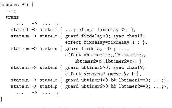
Figure 6 describes five transitionsA,B,C,D,EinPi (see the upper part of the figure) and their
asso-ciated timeline. TransitionA:stateidm -> stateidn has a fixed time delay,τ0; transitionB:stateidn -> stateido has upper and lower bounds, (τ2,τ1); transitionC: stateidn -> stateidp has upper and lower
bounds, (τ4,τ3). After the execution of transition A, there is a time period,(t3,t4), during which both
transitionBandCare enabled and chosen non-deterministically. TransitionD:stateido -> stateidqand E:stateidp -> stateidqhave the upper and lower bounds which are dependant on the execution time of BorC. The processPiin DVE is described in Figure 7.
3.3 An Example of Pre-emptive Scheduling
Figure 6: States and timeline for complex timers using SEDM
process P i {
...; trans
... -> ... ;
state l -> state m { ...; effect fixdelay=τ0; },
state m -> state m { guard fixdelay>0; sync chan1?; effect fixdelay=fixdelay-1 ; }, state m -> state n { guard fixdelay==0 ; ...;
effect ubtimer1=τ3,lbtimer1=τ1,
ubtimer2=τ4,lbtimer2=τ2; },
state n -> state n { guard ubtimer2>0; sync chan1?; effect decrement timers by 1;},
state n -> state o { guard ubtimer1>0 && lbtimer1==0; ...;}, state n -> state p { guard ubtimer2>0 && lbtimer2==0; ...;},
... -> ... ;
}
Figure 7: System processPiin DVE with complex timers
Figure 8 shows a portion of a state transition diagram for task A, assumingA needs the exclusive resource R for 10 time units; when R becomes available at time instant t0, A starts its execution by
entering the stateExec; at time instantt1,BdeprivesA’s right toR, andAchanges to the stateDeprived
and stores the elapsedt1−t0 time units; when R becomes available again,A resumes its execution to
stateExecfor the remaining 10−(t1−t0) units. Implementation of this example using any one of the
Figure 8: An Example of Pre-emptive Scheduling
byte isROccupied=0; //0 means available process A {
default(Tag,tagA)
int timeToGo=10;
state s i, s Exec, s Deprived, ...; init ...;
trans
... -> ... ;
s i -> s Exec { guard isROccupied==0;
effect isROccupied=Tag, ltimer=timeToGo; s Exec -> s Exec { guard ltimer>0; sync chan1?;
effect ltimer=ltimer-1; },
s Exec -> s Deprived { guard isROccupied=Tag && ltimer>0; effect timeToGO=ltimer; },
s Deprived -> s Deprived { guard isROccupied!=0; sync chan1?; }
s Deprived -> s Exec { guard isROccupied==0;
effect isROccupied=Tag, ltimer=timeToGo; }, s Exec -> s Next { guard ltimer==0;
effect isROccupied=0; }, ... -> ... ;
}
Figure 9: Process in DVE for Pre-emptive Scheduling Example using SEDM
4
Experiments in
D
IV
INE
[16]. The brief description of the algorithm is adapted from [16]. Our experiments model the algorithm in DIVINE using LEDM and SEDM, and compare the time and memory efficiency and size of state space.
Fischer’s algorithm is a shared-memory, multi-threaded algorithm. It uses a shared variablexwhose value is either a thread identifier (starting from 1) or zero; its initial value is zero. For the convenience of specification of the safety property in our experiments, we use a countercto count the number of threads that are in the critical section. The program for threadtis described in Figure 10.
ncs: noncritical section;
a:wait untilx= 0;
b:x:=t;
c:ifx6=tthen gotoa;
cs: critical section;
d:x:= 0;gotoncs;
Figure 10: Program of threadtin Fischer’s algorithm
The timing constraints are, first, that stepbmust be executed at mostδ time units (as a upper bound) after the preceding execution of stepa; and second, that stepccannot be executed until at least ε time units (as a lower bound) after the preceding execution of stepb. For step c, there is an additional upper bound εupper to ensure fairness. For convenience, we use the same value for three constraints, i.e.,
δ =ε =εupper =T. The algorithm is tested for 6 threads. The safety property, “no more than one
process can be in the critical section”, is specified asG(c<2)for the model.
LEDM SEDM
T States Time Memory States Time Memory 2 644987 1.8 4700.1 1838586 2.9 4865.3 4 3048515 3.3 4942.8 6923088 4.3 5641.9 6 11201179 7.2 6343.4 18460632 9.3 7402.0 8 32952899 18.6 9958.9 48177552 21.2 11905.0 10 82428155 49.2 18016.2 113914104 46.1 21894.8 12 182767747 115.0 34906.3 244265616 108.8 41454.5 14 369377435 290.9 65205.1 482259672 230.0 78936.2 16 693683459 617.5 122549.0 889586256 611.2 148010.0
Figure 11: Time (in seconds), number of states and memory usage (in MB) for Fischer’s algorithm using two explicit-time methods in DIVINE with 16 CPUs
The version 0.8.1 of the DIVINE-Cluster is used. This version has the new feature of pre-compiling the model in DVE into dynamically linked C functions; this feature speeds up the state space generation significantly. According to the published experimental results of DIVINE [19], we choose the OWCTY (One Way to Catch Them Young) algorithm for better time efficiency as our example property is known to hold.
Figure 11 compares time and memory efficiency for the two explicit-time description methods in both versions of DIVINE with 16 CPUs; it also shows how the size of state spaces increase asTincreases.
While SEDM has the bigger number of states for all models, as the model becomes larger, the time increases more slowly than with LEDM: time increases by a factor of 343 as T increases from 2 to 16 with LEDM; time increases by a factor of 204 asT increases from 2 to 16 with SEDM; It is also interesting to find that starting fromT=10, the time spent with SEDM islessthan the time with LEDM. Because SEDM addsN synchronization steps (recall thatN is the number of system processes) for each time units, the size of state space of the model generated by our method is bigger than that by Lamport’s method. But as the model becomes bigger, the difference becomes insignificant. ForT =2,
states(SEDM)
states(LEDM)=2.85, while forT =16, the two numbers of state size become comparable.
The memory usages of both methods are comparable. Because OWCTY algorithm requires that the whole state space fit into the (distributed) memory, enough memory resource must be allocated in order for the verification to succeed.
Note that when increasing the number of CPUs an added portion of memory needs to be counted for increasing inter-node communications.
5
Discussion and Conclusion
In this paper, we propose a new method, SEDM using rendezvous synchronization steps, so the timing constraints can be defined either globally or locally, compared to the heavy reliance on global variables in LEDM. Consequently, SEDM makes it possible to model discrete time with some process-based untimed languages without explicit global variables. With SEDM, real-time systems can be modeled with a high degree of modularity and more complex timing constraints can be modeled more conveniently.
As Lamport mention in [16], the explicit-time description methods are not designed to beat special-ized timed model checkers like UPPAAL: it is obvious that time-automata-based model checkers can handle continuous time semantics while EDMs can only deal with discrete time semantics. However, EDMs are intended to offer more options for the verification of real-time systems. First, explicit-time description methods provide a solution for accessing and storing the current time instant for the pre-emptive scheduling models. Second, while the size of state space in an explicit-time method grows along with the number of time units, it is less sensitive to the number of concurrently running timers. This suggests that the explicit-time method implemented in an un-timed model checker may verify more complex system behaviors. Third, as Van den Berg et al. mention in [10], in some real-world scenarios when significant resources already have been invested into the model for a general model checker such as SPIN or SMV, it is much easier and therefore preferable to extend the existing model to represent time notions rather than to re-model the entire system for a specialized timed model checker. Last but not least, explicit-time description methods enable the usage of existing large-scale distributed model checkers such as DIVINE so that we can verify much bigger real-time systems.
methods to model and verify real-world health care processes.
As a continuous effort in practical timed model checking, we also study the efficiency problem of explicit-time descriptions and have made some progress based on optimizing the tick process [20], so that EDMs can be applied to problems of larger scale. Dutertre and Sorea [13] and Clarke et al. [11] recently presented two different abstraction techniques for timed automata and the abstraction outcome can be verified using un-timed model checkers. We also intend to study the possibility of this kind of technique in distributed model checkers.
Acknowledgment
This research is sponsored by NSERC, an Atlantic Computational Excellence Network (ACEnet) Post Doctoral Research Fellowship and by the Atlantic Canada Opportunities Agency through an Atlantic Innovation Fund project. The computational facilities are provided by ACEnet. We also thank Jiri Barnat, Keith Miller and the anonymous reviewers of QFM’09 for their helpful comments.
References
[1] Atlantic Computational Excellence network (ACEnet). http://www.ace-net.ca/. Last accessed on Nov.2009. [2] Centre for Logic and Information, St. Francis Xavier University. http://logic.stfx.ca/. Last accessed on Nov.
2009.
[3] DIVINEproject. http://divine.fi.muni.cz/. Last accessed on Nov.2009.
[4] Yasmina Abdedda¨ım & Oded Maler (2002):Preemptive Job-Shop Scheduling Using Stopwatch Automata. In: Joost-Pieter Katoen & Perdita Stevens, editors:TACAS,Lecture Notes in Computer Science2280. Springer, pp. 113–126.
[5] Rajeev Alur & David L. Dill (1994):A Theory of Timed Automata.Theor. Comput. Sci.126(2), pp. 183–235. [6] Rajeev Alur & Thomas A. Henzinger (1991):Logics and Models of Real Time: A Survey. In: J. W. de Bakker, Cornelis Huizing, Willem P. de Roever & Grzegorz Rozenberg, editors: REX Workshop,Lecture Notes in Computer Science600. Springer-Verlag, pp. 74–106.
[7] Jiri Barnat, Lubos Brim, Ivana ˇCern´a, Pavel Moravec, Petr Roˇckai & Pavel ˇSimeˇcek (2006): DiVinE – A Tool for Distributed Verification (Tool Paper). In:Computer Aided Verification,Lecture Notes in Computer Science4144. Springer-Verlag, pp. 278–281.
[8] Johan Bengtsson, Kim G. Larsen, Fredrik Larsson, Paul Pettersson & Wang Yi (1995): UPPAAL— a Tool Suite for Automatic Verification of Real–Time Systems. In:Proc. of Workshop on Verification and Control of Hybrid Systems III, number 1066 in Lecture Notes in Computer Science. Springer-Verlag, pp. 232–243. [9] Johan Bengtsson & Wang Yi (2003): Timed Automata: Semantics, Algorithms and Tools. In: J¨org Desel,
Wolfgang Reisig & Grzegorz Rozenberg, editors:Lectures on Concurrency and Petri Nets,Lecture Notes in Computer Science3098. Springer, pp. 87–124.
[10] Lionel van den Berg, Paul A. Strooper & Kirsten Winter (2007):Introducing Time in an Industrial Appli-cation of Model-Checking. In: Stefan Leue & Pedro Merino, editors: FMICS,Lecture Notes in Computer Science4916. Springer, pp. 56–67.
[11] Edmund M. Clarke, Flavio Lerda & Muralidhar Talupur (2007): An Abstraction Technique for Real-time Verification. In: S. Ramesh & P. Sampath, editors:Next Generation Desigh and Verification Methodologies, Lecture Notes in Computer Science. Springer-Verlag, pp. 1–17.
[13] Bruno Dutertre & Maria Sorea (2004): Modeling and Verification of a Fault-Tolerant Real-Time Startup Protocol Using Calendar Automata. In: Yassine Lakhnech & Sergio Yovine, editors:FORMATS/FTRTFT, Lecture Notes in Computer Science3253. Springer-Verlag, pp. 199–214.
[14] Gerard J. Holzmann (1991):Design and Validation of Computer Protocols. Prentice Hall.
[15] Pavel Krc´al & Wang Yi (2004): Decidable and Undecidable Problems in Schedulability Analysis Using Timed Automata. In: Kurt Jensen & Andreas Podelski, editors:TACAS,Lecture Notes in Computer Science 2988. Springer, pp. 236–250.
[16] Leslie Lamport (2005):Real-Time Model Checking is Really Simple. In: Dominique Borrione & Wolfgang J. Paul, editors:CHARME,Lecture Notes in Computer Science3725. Springer-Verlag, pp. 162–175.
[17] Ken L. McMillan (1992): Symbolic model checking - an approach to the state explosion problem. Ph.D. thesis, Carnegie Mellon University.
[18] Moshe Y. Vardi & Pierre Wolper (1986):An Automata-Theoretic Approach to Automatic Program Verifica-tion (Preliminary Report). In:LICS. IEEE Computer Society, pp. 332–344.
[19] Kees Verstoep, Henri E. Bal, Jiri Barnat & Lubos Brim (2009): Efficient large-scale model checking. In: IPDPS. IEEE, pp. 1–12.