L. Brim and J. van de Pol (Eds.): 8th International Workshop on Parallel and Distributed Methods in verifiCation 2009 (PDMC’09) EPTCS 14, 2009, pp. 77–91, doi:10.4204/EPTCS.14.6
c
H. Wang & W. MacCaull This work is licensed under the Creative Commons Attribution License.
Model Checking
Hao Wang and Wendy MacCaull Centre for Logic and Information
St. Francis Xavier University Antigonish, Canada {hwang, wmaccaul}@stfx.ca
Timedmodel checking, the method to formally verify real-time systems, is attracting increasing atten-tion from both the model checking community and the real-time community.Explicit-time descrip-tion methodsverify real-time systems using general model constructs found in standard un-timed model checkers. Lamport proposed an explicit-time description method [17] using a clock-ticking process (Tick) to simulate the passage of time together with a group of global variables to model time requirements. Two methods, theSync-based Explicit-time Description Method using rendezvous synchronization steps and theSemaphore-based Explicit-time Description Methodusing only one global variable were proposed [27, 26]; they both achieve bettermodularitythan Lamport’s method in modeling the real-time systems. In contrast to timed automata based model checkers like UPPAAL [7], explicit-time description methods can access and store the current time instant for future calcula-tions necessary for many real-time systems, especially those with pre-emptive scheduling. However, theTickprocess in the above three methods increments the time by one unit in each tick; the state spaces therefore grow relatively fast as the time parameters increase, a problem when the system’s time period is relatively long. In this paper, we propose a more efficient method which enables the
Tickprocess to leap multiple time units in one tick. Preliminary experimental results in a high perfor-mance computing environment show that this new method significantly reduces the state space and improves both the time and memory efficiency.
1
Introduction
Model checking is an automatic analysis method which explores all possible states of a modeled system to verify whether the system satisfies a formally specified property. It was popularized in industrial applications, e.g., for computer hardware and software, and has great potential for modeling complex and distributed business processes.Timedmodel checking, the method to formally verify real-time systems, is attracting increasing attention from both the model checking community and the real-time community. However, standard model checkers like SPIN [15] and SMV [19] can generally only represent and verify the qualitative relations between events, which constrains their use for real-time systems. Quantified
time notions, including time instant and duration, must be taken into account for timed model checking. For example in a safety critical application such as in an emergency department, after an emergency case arrives at the hospital, standard model checking can only verify whether “the patient receives a certain treatment”, but to save the patient’s life, it should be verified whether “the patient receives a certain treatment within 1 hour”.
time Petri Nets to timed automata [22] in order to apply time-automata-based methods to time Petri Nets. UPPAAL [7] and KRONOS [28] are two well-known timed automata based model checkers; they have been successfully applied to various real-time controllers and communication protocols. Conventional temporal logics likeLinear Temporal Logic(LTL) orComputation Tree Logic(CTL) must be extended [5] to handle the specification of properties of timed automata. In order to handle continuous-time se-mantics, specialized data structures are needed to represent real clock variables, e.g. Difference Bounded Matrices [12] (employed by UPPAAL and KRONOS).
The foundation for the decidability results in timed automata is based on the notion ofregion equiva-lenceover the clock assignment [8]. Models in a timed automata based model checker can not represent at which time instant a transition is executed within a time region; such model checkers can only deal with a specification involving a time region or a pre-specified time instant and cannot store the exact time instant when the transition is executed. However, many real-time systems, especially those with pre-emptive scheduling, need this information for succeeding calculations. For example, triage is widely practiced in medical procedures; the caregiverC may be administering some required but non-critical treatment on patientAwhen another patientBpresents with a critical situation, such as a cardiac arrest.
Cthen must move to the higher priority task of treating B, but it is necessary to store the elapsed time ofA’s treatment to determine how much time is still needed or else the treatment must be restarted. The
stop-watch automata [3], an extension of timed automata, is proposed to tackle this; unfortunately as Krc´al and Yi discussed in [16], since the reachability problem for this class of automata is undecidable, there is no guarantee for termination in the general case.
Lamport [17] advocatedexplicit-time description methodsusing general model constructs, e.g., global integer variables or synchronization between processes commonly found in standard un-timed model checkers, to realize timed model checking. He presented an explicit-time description method, which we refer to as LEDM, using a clock-ticking process (Tick) to simulate the passage of time, and a pair of global variables to store the time lower and upper bounds for each modeled system process. The method has been implemented with popular model checkers SPIN (sequential) and SMV. We presented two methods, (1) theSync-based Explicit-time Description Method(SEDM) [27] using rendezvous syn-chronization steps between the Tick and each of the system processes; and (2) the Semaphore-based Explicit-time Description Method(SMEDM) [26] using only one global semaphore variable. Both these methods enable the time lower and upper bounds to be defined locally in system processes so that they provide bettermodularityin system modeling and facilitate the use of more complex timing constraints. Our experiments [26, 27] showed that the time and memory efficiencies of these two methods are com-parable to that of LEDM.
The explicit-time description methods have three advantages over timed-automata-based model check-ers: (1) they do notneed specialized languages or tools for time description so they can be applied in standard un-timed model checkers. Recently, Van den Berg et al. [9] successfully applied LEDM to ver-ify the safety of railway interlockings for one of Australia’s largest railway companies; (2) they enable the accessing and storing of the current time [26], a useful feature for pre-emptive scheduling problems; and (3) they enable the usage of large-scale distributed model checkers, e.g., DIVINE, for timed model checking.
of the system model; parallel processing of the states can, moreover, reduce the verification time. Our experiments [27] compared the time efficiency between the sequential SPIN and DIVINE [2], a well-known distributed model checker. When using the same explicit-time description method, DIVINE can verify much larger models and finish the verification for models of the same size in significantly less time than SPIN.
In this paper, we present a new explicit-time description method called Efficient Explicit-time De-scription Method (EEDM). We found that the former three methods (LEDM, SEDM and SMEDM) suffer from one common problem: as the Tick process increments the time by one unit in each tick, the state space grows relatively fast as the time parameters increase. E.g., in our experiment [26] using LEDM, the number of states doubles as time bounds grow from 12 to 14. In the new EEDM, theTick
can increment the time in two modes: thestandard mode and theleapingmode. When it is necessary to store the current time to allow access for future calculations, it ticks in the standard mode; otherwise, it ticks in the leaping mode. For each system process, we define one global variable indicating whether the process needs to store and access the current time, allowing theTickprocess to switch between the standard mode and the leaping mode. For the experiments, we continue using DIVINE (the method is also applicable to other standard model checkers); the results show that: in the leaping mode, the number of states can be reduced significantly, so it is much less affected by the increase of time parameters; in the standard mode, the time and memory efficiencies are comparable with the former methods.
The remainder of the paper is organized as follows. Section 2 gives background information with re-spect to the DIVINE model checker. The new explicit-time description method implemented in DIVINE is presented in Section 3; for comparison, LEDM is also briefly described in the same section. Section 4 describes our experiments and the results. Section 5 concludes the paper.
2
Preliminaries
Section 2.1 is adapted from [25]; the syntax outlined in Section 2.2, while incomplete, is meant for the presentation of the time-explicit description methods; the complete description can be found in [2].
2.1 Distributed Model Checking Algorithms inDIVINE
DIVINE is an explicit-state LTL model checker based on the automata-based procedure by Vardi and Wolper [24]. The property to be specified is described by an LTL formula. In LTL model checking, all efficientsequentialalgorithms are based on the postorder exploration as computed by a depth-first search (DFS) of the state space. However, computing DFS postorder is P-complete [23], so no benefit in terms of either time or space will result from parallelization of this type of algorithm.
Two algorithms, OWCTY and MAP [6], are introduced in DIVINE. The sequential complexity of each is worse than that of the DFS-based algorithms but both can be efficiently implemented in parallel. OWCTY, orOne Way to Catch Them Young, is based on the fact that a directed graph can be topologically sorted if and only if it is acyclic. The algorithm applies a standard linear topological sort algorithm to the graph. Failure in the sorting means the graph contains a cycle. Accepting cycles are detected with multiple rounds of the sorting. MAP, or Maximal Accepting Predecessors, is based on the fact that each accepting vertex in an accepting cycle is its own predecessor. To improve memory efficiency, the algorithm only stores a single representative accepting predecessor for each vertex by choosing the maximal one in a linear ordering of vertices.
and the state space can fit completely into (distributed) memory, OWCTY is preferable as it is three times faster than MAP to explore the whole state space. On the other hand, MAP can generally find a counterexample (if it exists) more quickly as it works on-the-fly.
2.2 DIVINE Modeling Language
DVE is the modeling language of DIVINE. Like in Promela (the modeling language of SPIN), a model described in DVE consists of processes, message channels and variables. Each process, identified by a unique nameprocid, consists of lists of local variable declarations and state declarations, the initial state declaration and a list of transitions.
A transition transfers the process state fromstateid1tostateid2. The transition may contain a guard (which decides whether the transition can be executed), a synchronization (which communicates data with another process) and an effect (which assigns new values to local or global variables). So we have
Transition ::= stateid1 -> stateid2 { Guard Sync Effect }
TheGuardcontains the keywordguardfollowed by a boolean expression and theEffectcontains the keywordeffectfollowed by a list of assignments. TheSyncfollows the denotation for communi-cation in CSP, ‘!’ for the sender and ‘?’ for the receiver. The synchronization can be either asynchronous or rendezvous. Value(s) is transferred in the channel identified bychanid. So we have
Sync ::= sync chanid ! SyncValue | chanid ? SyncValue ;
A property process is automatically generated for the corresponding property written as an LTL formula. Modeled system processes and the property process progress synchronously, so the latter can observe the system’s behavior step by step and catch errors.
3
Explicit-Time Description Methods
With explicit-time description methods, the passage of time and timed quantified values can be expressed in un-timed languages and properties to be specified can be expressed in conventional temporal logics. This section describes Lamport’s LEDM before detailing our new EEDM. At the end of this section, we study a small pre-emptive example with respect to explicit-time description methods.
3.1 The Lamport Explicit-time Description Method
In LEDM, current time is represented with a global variablenowthat is incremented by an addedTick
process. As we mentioned earlier, standard model checkers can only deal with integer variables, and a real-time system can only be modeled in discrete-time using an explicit-time description. So theTick
process incrementsnowby 1. Note that in explicit-time description methods for standard model check-ers, the real-valued time variables must be replaced by integer-valued ones. Therefore, these methods in general do not preserve the continuous-time semantics; otherwise an inherently infinite-state specifica-tion will be produced and the verificaspecifica-tion will be undecidable. However, they are sound for a commonly used class of real-time systems and their properties [14].
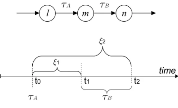
Figure 1: States and Timeline of processPi
τA:stateidl -> stateidmis followed by the transitionτB:stateidm -> stateidn. An upper-bound timing constraint on when transitionτBmust occur is expressed by a guard on the transition in theTickprocess so as to prevent an increase in time from violating the constraint. A lower-bound constraint on when transitionτB may occur is expressed by a guard onτB so it cannot be executed earlier than it should be. Each system processPihas a pair of count-down timers denoted as global variablesubtimeriandlbtimeri for the timing constraints on its transitions. A large enough integer constant, denoted asINFINITY, is defined. All upper bound timers are initialized toINFINITYand all lower bound timers are initialized to zero. Upper bound timers with the value ofINFINITYare not active and the Tick process will not decrement them. For transitionτB, the timers will be set to the correct values byτA:stateidl -> stateidm. Asnowis incremented by 1, each non-INFINITY ubtimerand non-zerolbtimeris decremented by 1.
process P Tick {
state tick; init tick; trans
tick -> tick { guard all ubtimers > 0; effect now = now + 1,
decrements all timers; } ;
}
Figure 2:Tickprocess in DVE for LEDM
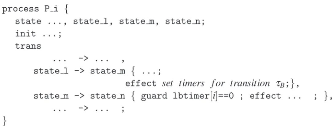
In Figure 1, initially, (ubtimeri,lbtimeri)is set to(INFINITY,0). TransitionτA is executed at time instant t0, and (ubtimeri,lbtimeri) is set to(ξ2,ξ1). After ξ1 time units, i.e., at time instant t1 when (ubtimeri,lbtimeri)is equal to(ξ2−ξ1,0), transitionτB is enabled. Both timers will be reset or set to new time bounds after the execution ofτB. If transitionτB is still not executed when the time reachest2 andubtimeri is equal to 0, the transition in theTickprocess is disabled. This forces transitionτB (it is the only transition possible at this time) to set theubtimeri; then theTickprocess can start again. In this way, the time upper-bound constraint is realized. TheTickprocess and the system processPiin DVE are described in Figure 2 and Figure 3.
process P i {
state ..., state l, state m, state n; init ...;
trans
... -> ... ,
state l -> state m { ...;
effect set timers f or transition τB;},
state m -> state n { guard lbtimer[i]==0 ; effect ... ; }, ... -> ... ;
}
Figure 3: System processPiin DVE for LEDM
now= (now+1)mod MAXIMAL(MAXIMALis the maximal integer value supported by the model checker). The value limit can also be increased by linking several integers, i.e., every time(int1+1) mod MAXIMAL becomes zero again,int2increments by 1, and so on. Note that the variablenowis only incremented in theTickprocess and does not appear in any other process. So for general system models in which time lower and upper bounds suffice, the variablenowshould be removed.
3.2 The New Efficient Explicit-Time Description Method
This section is organized as follows. First, we describe the leaping mode and the standard mode of the new EEDM in section 3.2.1 and 3.2.2 respectively. Second, we present some discussions (clarifications) of issues on EDMs and EEDM in section 3.2.3. Finally, a pre-emptive scheduling modeling example using EEDM is described in section 3.2.4.
3.2.1 Leaping Ticks
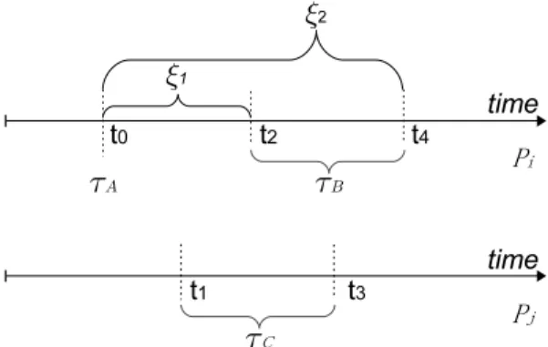
All aforementioned explicit-time description methods (LEDM, SEDM and SMEDM) increasenow by 1 each tick. On the other hand, consider Figure 4: we observe that when the system contains onlyone process, Pi, after t0, τB cannot be executed until time reaches t2. Therefore, the ticks between t0 and
t1 serve no purpose; optimally, the Tick process should directly “leap” tot2. Similarly, τB is enabled between t2 and t4, so either τB is executed before t4 or time reaches t4 and τB’s execution is forced; therefore, theTickprocess can leap tot4fromt2. When we includePj, aftert0, theTickshould first leap tot1soPjcan enable transitionτC; then it should leap tot2and so on.
Based on these observations, in the new EEDM, we use one global count-down timer for each system process, e.g.,timeri forPiin Figure 4 is set toξ1ont0and toξ2−ξ1ont2. TheTickprocess increments
nowby the value of the smallest timer on condition that no timer equals zero and at least one timer is non-INFINITY. In fact, theTickprocess, leaping in this way, is running in the leapingmode; theTick
process in leaping mode and the corresponding system processPiin DVE are described in Figure 5 and Figure 6 (Nis the number of system processes).
3.2.2 To Know the Current Time Instant
Figure 4: Timeline of processPiandPj
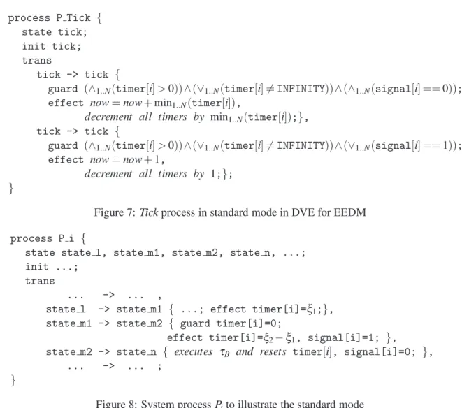
process P Tick {
state tick; init tick; trans
tick -> tick { guard (∧1..N(timer[i]>0))∧(∨1..N(timer[i]6=INFINITY));
effect now=now+min1..N(timer[i]),
decrement all timers by min1..N(timer[i]);};
}
Figure 5:Tickprocess in leaping mode in DVE for EEDM
process P i {
state state l, state m1, state m2, state n, ...; init ...;
trans
... -> ... ,
state l -> state m1 { ...; effect timer[i]=ξ1;},
state m1 -> state m2 { guard timer[i]=0; effect timer[i]=ξ2−ξ1; },
state m2 -> state n { executes τB and resets timer[i]; },
... -> ... ;
}
Figure 6: System processPiin DVE for EEDM
executed between the two closest ticks that nest the transition. Consider the example in Figure 4; theTick
will sequentially leap fromt0throught4;τBmay be executed on: (1) some time instant betweent2andt3; or (2) some time instant betweent3andt4; or (3) the time instant oft4. However, as we discussed earlier in Section 1 and in [26], in many systems, especially those with pre-emptive scheduling, it is necessary to know the actual time instant when the transition is executed.
process P Tick {
state tick; init tick; trans
tick -> tick {
guard (∧1..N(timer[i]>0))∧(∨1..N(timer[i]6=INFINITY))∧(∧1..N(signal[i] ==0));
effect now=now+min1..N(timer[i]),
decrement all timers by min1..N(timer[i]);},
tick -> tick {
guard (∧1..N(timer[i]>0))∧(∨1..N(timer[i]6=INFINITY))∧(∨1..N(signal[i] ==1));
effect now=now+1,
decrement all timers by 1;};
}
Figure 7: Tickprocess in standard mode in DVE for EEDM
process P i {
state state l, state m1, state m2, state n, ...; init ...;
trans
... -> ... ,
state l -> state m1 { ...; effect timer[i]=ξ1;},
state m1 -> state m2 { guard timer[i]=0;
effect timer[i]=ξ2−ξ1, signal[i]=1; },
state m2 -> state n { executes τB and resets timer[i], signal[i]=0; },
... -> ... ;
}
Figure 8: System processPito illustrate the standard mode
in turn will run in the standard mode with which it will increment nowby 1 in each tick. E.g., when time reachest2 in Figure 4,Pi’s signalsignali is set to 1 in order to store the time instant at whichτBis executed; when time reachest4,signali is set back to 0 so that theTickswitches back to leaping mode. Both theTickprocess and the system process need to be updated to incorporate the standard mode, see Figure 7 and Figure 8.
3.2.3 Issues on EDMs and EEDM
Readers may be concerned about the verification capability of explicit-time description methods. As in our earlier discussion, EDMs simulate adiscretetimer by making use of existing constructs in standard un-timed model checkers; in other words, time is just another normal variable in an un-timed model. Therefore, EDMs are not affected by verification issues such as whether the property is specified as an LTL or CTL formula or whether the property is verified using explicit-state based (e.g., Spin) or symbolic model checking (e.g., SMV) algorithms. These verification issues depend on what standard un-timed model checker is used.
(granularity) that does not mask errors. E.g., for processes in a hospital, a time unit defined as a day will definitely mask an error which violates the property “the patient receives a certain treatment within 1 hour”. On the other hand, the state space can easily blow up if a finer time unit is used. Readers may be concerned that the introduction of leaping ticks may add to this problem. Actually, leaping ticks do not musk errors in this aspect. The difference between LEDM and EEDM in leaping mode is that EEDM in leaping mode cannot record and use the exact time instant when a transition is executed in the model or the specified properties. For example, the LTL property that b becomes true before 10 time units have elapsed sinceτBis executed cannot be verified using EEDM in leaping mode. For this reason, we introduce the mode-switching mechanism in EEDM.
To reduce the state space, Lamport [17] proposed the use of view symmetry, which is equivalent to abstraction for a symmetric specification S. Abstraction consists of checking S by model checking a different specification A called an abstraction ofS. This technique has two restrictions: (1) the now
variable must be eliminated, which means the current time instant is not accessible in this case; (2) if the model checker does not support checking under view symmetry or abstraction, the abstraction specificationAmust be constructed by hand. In addition, this reduction technique is orthogonal to our EEDM, i.e., we can use Lamport’s abstraction technique in conjunction with EEDM.
The idea of leaping ticks in EEDM is quite similar to the notion of time regions in time-automata-based model checkers, which advances time up to the point where a transition must be executed in order not to violate the invariant defined on the corresponding state. However, the implementations are fundamentally different: time-automata-based model checkers introduce specialized data structures [16] to store time regions and use symbolic model checking algorithms extended for time; on the other hand, EEDM, as with LEDM, only uses an explicittick process and some global variables, and the leaping way of advancing time is obtained by letting the tick leap to the next closest time bound of all systems processes.
3.2.4 To Know The Current Time Instant: A Pre-emptive Scheduling Example
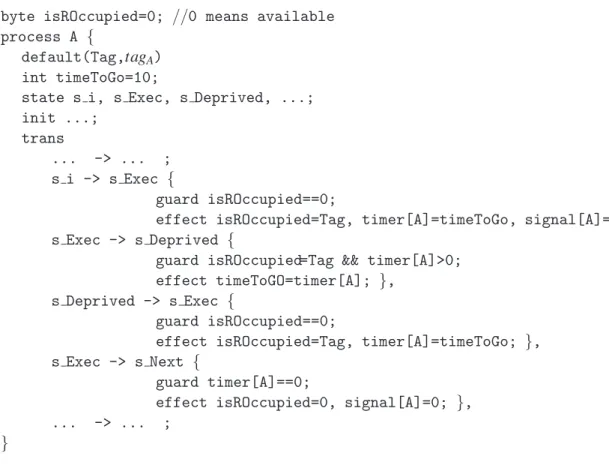
Following the triage example described in Section 1, we consider a system of multiple parallel tasks with different priorities, assuming that the right to an exclusive resource is deprivable, i.e., a higher priority taskBmay deprive the resource from the currently running taskA. In this case, the elapsed time ofA’s execution must be stored for a future resumed execution.
Figure 9 shows a portion of a state transition diagram for task A, assumingA needs the exclusive resource R for 10 time units; when R becomes available at time instant t0, A starts its execution by entering the stateExec; at time instantt1,BdeprivesA’s right toR, andAchanges to the stateDeprived and stores the elapsedt1−t0time units; whenRbecomes available again,Aresumes it execution to state
Execfor the remaining 10−(t1−t0)units. Implementation of this example using any one of the three explicit-time description methods is straightforward. Figure 10 shows the process for taskA in DVE using EEDM (assumingAhas the lowest priority).
4
Experiments
4.1 Overview
Figure 9: An Example Case of Pre-emptive Scheduling
byte isROccupied=0; //0 means available process A {
default(Tag,tagA)
int timeToGo=10;
state s i, s Exec, s Deprived, ...; init ...;
trans
... -> ... ; s i -> s Exec {
guard isROccupied==0;
effect isROccupied=Tag, timer[A]=timeToGo, signal[A]=1; s Exec -> s Deprived {
guard isROccupied=Tag && timer[A]>0; effect timeToGO=timer[A]; },
s Deprived -> s Exec {
guard isROccupied==0;
effect isROccupied=Tag, timer[A]=timeToGo; }, s Exec -> s Next {
guard timer[A]==0;
effect isROccupied=0, signal[A]=0; }, ... -> ... ;
}
Figure 10: Process in DVE for Pre-emptive Scheduling Example using EEDM
Fischer’s algorithm is a shared-memory, multi-threaded algorithm. It uses a shared variablexwhose value is either a thread identifier (starting from 1) or zero; its initial value is zero. For the convenience of specification of the safety property in our experiments, we use a countercto count the number of threads that are in the critical section. The program for threadtis described in Figure 11.
ncs: noncritical section;
a:wait untilx= 0;
b:x:=t;
c:ifx6=tthen gotoa;
cs: critical section;
d:x:= 0;gotoncs;
Figure 11: Program of threadtin Fischer’s algorithm
The timing constraints are: first, stepbmust be executed at mostδbu time units (as an upper bound) after the preceding execution of stepa; second, stepccannot be executed until at leastδcl time units (as a lower bound) after the preceding execution of step b. For step c, there is an additional upper bound
δu
c to ensure fairness, i.e., stepcwill eventually be executed. The algorithm is tested for 6 threads. The safety property to be verified,“no more than one process can be in the critical section”, is specified as
G(c<2)for the model.
Version 0.8.1 of the DIVINE-Cluster is used. This version has the new feature of pre-compiling the model in DVE into dynamically linked C functions; this feature speeds up the state space generation significantly. As the example property is known to hold, the OWCTY algorithm is chosen for better time efficiency.
All experiments are executed on the Mahone cluster of ACEnet [1], the high performance computing consortium for universities in Atlantic Canada. The cluster is a Parallel Sun x4100 AMD Opteron (dual-core) cluster equipped with Myri-10G interconnection. Parallel jobs are assigned using the Open MPI library.
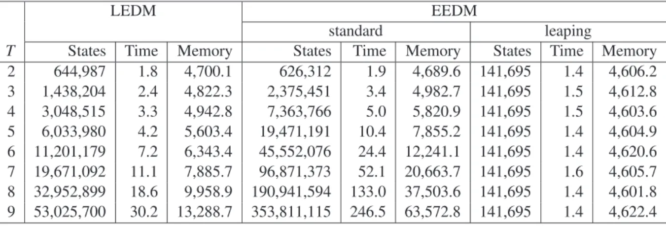
4.2 Experiment 1
For the first experiment, we use the same value for three constraints, i.e.,δbu=δl
c =δcu=T. Figure 12 compares time and memory efficiency for the two explicit-time description methods with 16 CPUs.
We can see the significant advantage of EEDM in leaping mode: the number of states, verification time and memory usage remain virtually the same for allTs. Remark that all timing bounds are the same for all threads; theTickprocess always leapsT time units in each tick (it ticks only when there is at least one active timer). Therefore, changing the value ofT will not change the number of states.
Now we compare LEDM and EEDM in standard mode. Letstates(X)be the number of states of methodX. We can see that, afterT =3,states(EEDMstandard)>states(LEDM). AsT increases from
2 to 9,states(EEDMstandard)increases by a factor of 564.9 whilestates(LEDM)increases by a factor
LEDM EEDM
standard leaping
T States Time Memory States Time Memory States Time Memory
2 644,987 1.8 4,700.1 626,312 1.9 4,689.6 141,695 1.4 4,606.2
3 1,438,204 2.4 4,822.3 2,375,451 3.4 4,982.7 141,695 1.5 4,612.8 4 3,048,515 3.3 4,942.8 7,363,766 5.0 5,820.9 141,695 1.5 4,603.6 5 6,033,980 4.2 5,603.4 19,471,191 10.4 7,855.2 141,695 1.4 4,604.9 6 11,201,179 7.2 6,343.4 45,552,076 24.4 12,241.1 141,695 1.4 4,620.6 7 19,671,092 11.1 7,885.7 96,871,373 52.1 20,663.7 141,695 1.6 4,605.7 8 32,952,899 18.6 9,958.9 190,941,594 133.0 37,503.6 141,695 1.4 4,601.8 9 53,025,700 30.2 13,288.7 353,811,115 246.5 63,572.8 141,695 1.4 4,622.4
Figure 12: Number of states, Time (in seconds) and memory usage (in MB) for Experiment 1
4.3 Experiment 2
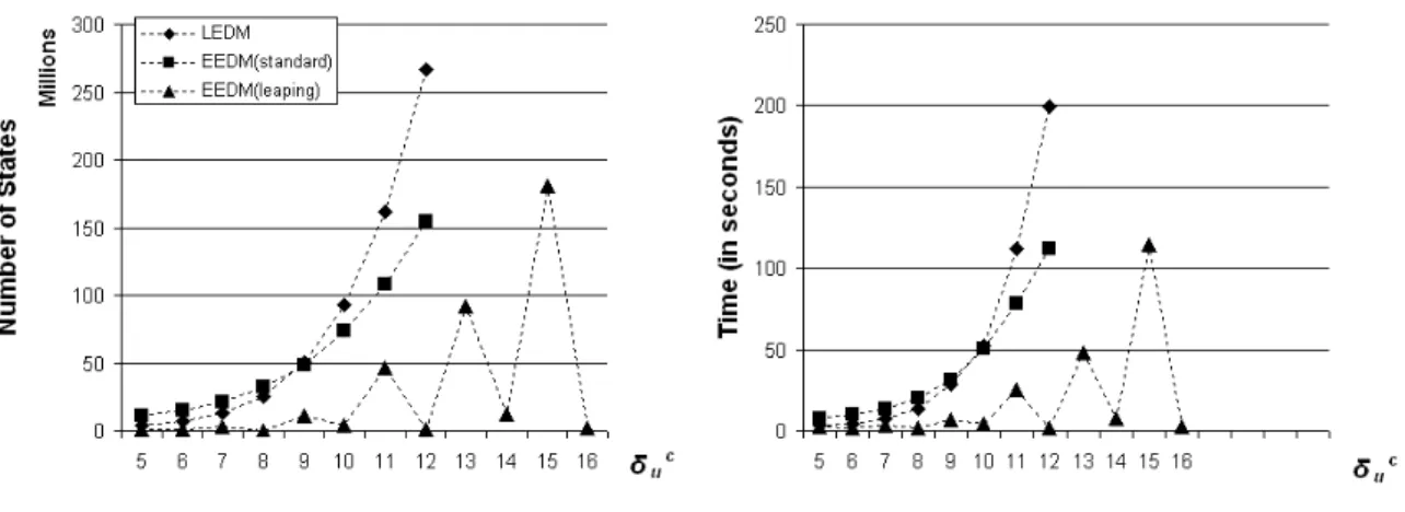
For the second experiment, we setδbuandδclto 4 and varyδcu. Figure 13 compares the number of states, time and memory efficiency for the two explicit-time description methods with 16 CPUs. Figure 14 shows how the size of the state space and verification time grow asδcuincreases. The extra experimental data forδcu={13,14,15,16}are intended to articulate the growing pattern of the state space of EEDM in leaping mode.
LEDM EEDM
Standard Leaping
δu
c States Time Memory States Time Memory States Time Memory
5 3,659,317 3.5 5,199.1 10,865,877 7.2 6,415.6 1,122,491 2.2 4,771.0 6 6,783,455 4.2 5,770.2 15,221,140 10.2 7,150.3 1,046,759 2.0 4,758.0 7 12,907,369 7.2 6,754.2 21,451,024 13.2 8,198.5 3,516,193 3.6 5,182.7 8 25,723,697 13.3 8,898.8 31,934,332 20.2 9,946.8 365,279 1.6 4,651.1 9 50,500,739 28.2 13,047.6 48,889,270 31.2 12,721.1 10,998,335 7.1 6,434.9 10 93,349,553 52.3 20,146.1 73,501,090 50.7 16,858.4 3,828,687 3.8 5,228.0 11 161,886,059 111.9 31,722.6 108,005,926 78.5 23,104.9 46,149,106 24.9 12,313.8 12 266,256,377 199.2 49,154.8 154,662,946 112.2 30,045.6 857,773 1.9 4,735.3
13 92,147,198 48.4 19,928.2
14 12,275,835 7.3 6,650.4
15 180,459,742 114.1 34,098.7
16 1,847,395 2.7 4,911.5
Figure 13: Number of states, Time (in seconds) and memory usage (in MB) for Experiment 2
As opposed to the results in experiment 1, in this experiment EEDM in standard mode performs better than LEDM. We can see that afterδcu=9,states(EEDMstandard)<states(LEDM); as the model
becomes larger, states(EEDMstandard) increases more slowly than states(LEDM). In fact, as δcu in-creases from 5 to 12,states(LEDM)increases by a factor of 72.8 whilestates(EEDMstandard)increases
Figure 14: Number of states and Time (in seconds) for Experiment 2
EEDM in leaping mode still shows much better performance than LEDM and EEDM in standard mode; states(EEDMleaping) also shows an interesting phenomenon as δcu increases. The number of states of both EEDM in standard mode and LEDM increase at a relatively more steady speed: asδcu in-creases by 1, states(EEDMstandard) increases by a factor of about 1.45 and states(LEDM)increases
by a factor of about 1.8. On the other hand, the increments of states(EEDMleaping) are grouped
by the value of s = (δu
c mod δcl). We can see that, for the same ⌊δ
u c
δl
c⌋, states(EEDMleaping)s=0 <
states(EEDMleaping)s=2<states(EEDMleaping)s=1<states(EEDMleaping)s=3. Fors=0, whenever
there is more than one active timer, their values are integer multiples ofδcl (4 in this experiment), so the
Tickstill leaps at least 4 time units each tick; in the case ofs=2, theTickleaps at least 2 time units each tick. On the other hand, fors=1 ands=3, in the worst case, theTickleaps only 1 time units each tick. From these observations, we can conclude that EEDM in leaping mode performs better the greater the
greatest common divisor(gcd) of all timing bounds of all system processes.
5
Conclusion
In this paper, we present a new explicit-time description method, Efficient Explicit-time Description Method (EEDM) which is significantly more efficient than LEDM, SEDM and SMEDM. In addition to the improved efficiency, EEDM still retains the ability to store and access the current time for future calculations in the system model. Altogether, we have devised methods that have advantages in different aspects of real-time modeling: SEDM and SMEDM have better modularity and adaptability; EEDM is more efficient. These explicit-time description methods provide systematic ways to represent discrete time in un-timed model checkers like SPIN, SMV and DIVINE.
large-scale distributed model checkers so that we can verify much bigger real-time systems.
This research is part of an ambitious research and development project, Building Decision-support through Dynamic Workflow Systems for Health Care [21]. Real world workflow processes can be highly dynamic and complex in a health care setting. Verification that the system meets its specifications is essential. Standard workflow patterns are widely used in business processes modeling, so we have trans-lated most of the control-flow patterns into DVE and applied them in verifying two small process models [18]. As a continuous effort, we will incorporate explicit-time description methods into workflow pat-terns’ DVE specification and verify a larger model of the real-world healthcare processes with timing information.
As a more complex case study of EEDM, we are now building a pre-emptive scheduling model in the setting of the Dynamic Voltage Scaling (DVS) technique. We also plan to study the possibility of applying different abstraction techniques to the explicit-time description methods: Dutertre and Sorea [13] and Clarke et al. [11] recently presented two different abstraction techniques for timed automata and the abstraction outcome can be verified using un-timed model checkers.
Acknowledgment
This research is sponsored by Natural Sciences and Engineering Research Council of Canada (NSERC), an Atlantic Computational Excellence Network (ACEnet) Post Doctoral Research Fellowship and the Atlantic Canada Opportunities Agency (ACOA) through an Atlantic Innovation Fund project. The com-putational facilities are provided by ACEnet. We thank Jiri Barnat, Keith Miller and the anonymous reviewers of PDMC’09 for their valuable comments.
References
[1] Atlantic Computational Excellence network (ACEnet). http://www.ace-net.ca/. Last accessed on Nov.2009.
[2] DIVINEproject. http://divine.fi.muni.cz/. Last accessed on Nov.2009.
[3] Yasmina Abdedda¨ım & Oded Maler (2002):Preemptive Job-Shop Scheduling Using Stopwatch Automata. In: Joost-Pieter Katoen & Perdita Stevens, editors:TACAS,Lecture Notes in Computer Science2280. Springer-Verlag, pp. 113–126.
[4] Rajeev Alur & David L. Dill (1994):A Theory of Timed Automata.Theor. Comput. Sci.126(2), pp. 183–235. [5] Rajeev Alur & Thomas A. Henzinger (1991):Logics and Models of Real Time: A Survey. In: J. W. de Bakker, Cornelis Huizing, Willem P. de Roever & Grzegorz Rozenberg, editors: REX Workshop,Lecture Notes in
Computer Science600. Springer-Verlag, pp. 74–106.
[6] Jiri Barnat, Lubos Brim & Ivana Cern´a (2005): Cluster-Based LTL Model Checking of Large Systems. In: Frank S. de Boer, Marcello M. Bonsangue, Susanne Graf & Willem P. de Roever, editors: FMCO,Lecture
Notes in Computer Science4111. Springer-Verlag, pp. 259–279.
[7] Johan Bengtsson, Kim Guldstrand Larsen, Fredrik Larsson, Paul Pettersson & Wang Yi (1995): UPPAAL - a Tool Suite for Automatic Verification of Real-Time Systems. In: Rajeev Alur, Thomas A. Henzinger & Eduardo D. Sontag, editors:Hybrid Systems,Lecture Notes in Computer Science1066. Springer-Verlag, pp. 232–243.
[8] Johan Bengtsson & Wang Yi (2003): Timed Automata: Semantics, Algorithms and Tools. In: J¨org Desel, Wolfgang Reisig & Grzegorz Rozenberg, editors:Lectures on Concurrency and Petri Nets,Lecture Notes in
[9] Lionel van den Berg, Paul A. Strooper & Kirsten Winter (2007): Introducing Time in an Industrial Appli-cation of Model-Checking. In: Stefan Leue & Pedro Merino, editors: FMICS,Lecture Notes in Computer Science4916. Springer-Verlag, pp. 56–67.
[10] Lubos Brim (2004):Parallel Model Checking.ERCIM News2004(58), pp. 35–36.
[11] Edmund M. Clarke, Flavio Lerda & Muralidhar Talupur (2007): An Abstraction Technique for Real-time Verification. In: S. Ramesh & P. Sampath, editors:Next Generation Desigh and Verification Methodologies for Distributed Embedded Control Systems: Proceedings of the General Motors Research and Development
Workshop, Lecture Notes in Computer Science. Springer-Verlag, pp. 1–17.
[12] David L. Dill (1989): Timing Assumptions and Verification of Finite-State Concurrent Systems. In: Joseph Sifakis, editor:Automatic Verification Methods for Finite State Systems,Lecture Notes in Computer Science
407. Springer-Verlag, pp. 197–212.
[13] Bruno Dutertre & Maria Sorea (2004): Modeling and Verification of a Fault-Tolerant Real-Time Startup Protocol Using Calendar Automata. In: Yassine Lakhnech & Sergio Yovine, editors:FORMATS/FTRTFT,
Lecture Notes in Computer Science3253. Springer-Verlag, pp. 199–214.
[14] Thomas A. Henzinger, Zohar Manna & Amir Pnueli (1992): What Good Are Digital Clocks? In: Werner Kuich, editor:ICALP,Lecture Notes in Computer Science623. Springer-Verlag, pp. 545–558.
[15] Gerard J. Holzmann (1991):Design and Validation of Computer Protocols. Prentice Hall.
[16] Pavel Krc´al & Wang Yi (2004): Decidable and Undecidable Problems in Schedulability Analysis Using Timed Automata. In: Kurt Jensen & Andreas Podelski, editors:TACAS,Lecture Notes in Computer Science
2988. Springer-Verlag, pp. 236–250.
[17] Leslie Lamport (2005):Real-Time Model Checking Is Really Simple. In: Dominique Borrione & Wolfgang J. Paul, editors:CHARME,Lecture Notes in Computer Science3725. Springer-Verlag, pp. 162–175.
[18] Nazia Leyla, Ahmed Mashiyat, Hao Wang & Wendy MacCaull (2009):Workflow Verification with DiVinE.
In:Parallel and Distributed Methods in verifiCation, 8th International Workshop, PDMC 2009, Held as Part
of the Formal Methods Week 2009, Eindhoven, the Netherlands, November 2-6, 2009. Short paper.
[19] Ken L. McMillan (1992): Symbolic model checking - an approach to the state explosion problem. Ph.D. thesis, Carnegie Mellon University.
[20] Philip M. Merlin (1974): A study of the recoverability of computing systems. Ph.D. thesis, Department of Information and Computer Science, University of California, Irvine, CA.
[21] Keith Miller & Wendy MacCaull (2009): Toward Web-based Careflow Management Systems. Journal of
Emerging Technologies in Web Intelligence (JETWI)Special Issue, E-health: Towards System
Interoper-ability through Process Integration and Performance Management. Accepted.
[22] Wojciech Penczek & Agata P´olrola (2004): Specification and Model Checking of Temporal Properties in Time Petri Nets and Timed Automata. In: Jordi Cortadella & Wolfgang Reisig, editors: ICATPN,Lecture
Notes in Computer Science3099. Springer-Verlag, pp. 37–76.
[23] John H. Reif (1985):Depth-First Search is Inherently Sequential.Inf. Process. Lett.20(5), pp. 229–234. [24] Moshe Y. Vardi & Pierre Wolper (1986):An Automata-Theoretic Approach to Automatic Program
Verifica-tion (Preliminary Report). In:LICS. IEEE Computer Society, pp. 332–344.
[25] Kees Verstoep, Henri E. Bal, Jiri Barnat & Lubos Brim (2009): Efficient large-scale model checking. In:
IPDPS. IEEE, pp. 1–12.
[26] Hao Wang & Wendy MacCaull (2009): Timed Model Checking with Explicit-time Description Methods. Technical Report StFX-CLI-TR-2009-03, Centre for Logic and Information, St. Francis Xavier University. [27] Hao Wang & Wendy MacCaull (2009):Verifying Real-Time Systems using Explicit-time Description
Meth-ods. In:16th International Symposium on Formal Methods Workshop, Quantitative Formal Methods: Theory
and Applications, QFM 2009, Eindhoven, the Netherlands, November 3, 2009.