Predicting survival function and identifying
associated factors in patients with renal
insuiciency in the metropolitan area of
Maringá, Paraná State, Brazil
A predição da função de sobrevivência e identiicação
de fatores associados em pacientes renais
crônicos na área metropolitana de
Maringá, Paraná, Brasil
Prediciendo la esperanza de vida e identiicando
factores asociados en pacientes con insuiciencia
renal en el área metropolitana de Maringá,
Estado de Paraná, Brasil
Thiago G. Ramires 1
Luiz R. Nakamura 2
Ana J. Righetto 3
Edwin M. M. Ortega 3
Gauss M. Cordeiro 4
Abstract
Renal insufficiency is a serious medical and public health problem worldwide. Recently, although many surveys have been developed to identify factors re-lated to the lifetime of patients with renal insufficiency, controversial results from several studies suggest that researches should be conducted by region. Thus, in this study we aim to predict and identify factors associated with the lifetime of patients with chronic renal failure (CRF) in the metropolitan area of Maringá, Paraná State, Brazil, based on the generalized additive models for location, scale and shape (GAMLSS) framework. Data used in this study were collected from the Maringá Kidney Institute and comprehends 177 patients (classified with CRF and mostly being treated under the Brazilian Unified National Health System) enrolled in a hemodialysis program from 1978 up to 2010. By using this approach, we concluded that in other regions, gender, kid-ney transplant indicator, antibodies to hepatitis B and antibodies to hepatitis C are significant factors that affect the expected lifetime.
Survival Analysis; Renal Insufficiency; Kidney Diseases
Correspondence
L. R. Nakamura
Universidade Federal de Santa Catarina.
Campus Reitor João David Ferreira Lima s/n, Florianópois, SC 88040-900, Brasil.
1 Universidade Tecnológica Federal do Paraná, Curitiba, Brasil.
2 Universidade Federal de Santa Catarina, Florianópolis, Brasil. 3 Escola Superior de Agricultura Luiz de Queiroz, Universidade de São Paulo, Piracicaba, Brasil.
4 Universidade Federal de Pernambuco, Recife, Brasil.
Introduction
Renal failure, also known as renal insufficiency and kidney failure, is a serious medical and public health problem, characterized by the inability of the kidneys to excrete toxic substances from the body in a proper way 1. There are numerous causes of kidney failure. Some of them lead to a rapid decline
in renal function, with values less than 1 to 2% of normal levels, named acute renal failure (ARF). In addition, a gradual and progressive loss of a large part of the functioning nephrons can be observed, called chronic renal failure (CRF). According to Marques et al. 2, symptoms of kidney failure include
headache, weakness, anorexia, nausea, vomiting, cramps, diarrhea, oliguria (insufficient secretion of urine), edema, confusion, thirst, loss of smell and taste, somnolence, hypertension and tendency to hemorrhage resulting from renal failure, as well as skin pallor, xerosis (pathological skin dryness), dysmenorrhea (cramping before or during menstruation), amenorrhea (absence of menses), testicular atrophy, impotence, attention deficit disorder, muscle spasms, and coma.
Patients who, for some reason, lost their kidney function and irretrievably reached the terminal stage of the disease, now have three different methods for treatment: hemodialysis, peritoneal dialysis and kidney transplantation. According to the Brazilian Society of Nephrology, hemodialysis pro-motes the removal of toxic substances, water and minerals from the body by filtering the blood. It is generally held three times per week in sessions lasting an average of three up to four hours, with the aid of a machine, in specialized clinics.
De-Lima et al. 3 and Andrade et al. 4 report that despite various technological innovations
incor-porated in hemodialysis, Brazilian’s studies did not show any great improvement in survival of patients with CRF in recent decades. The lack of increased survival of CRF carriers maintained on kidney dialysis could be explained by the increase in the average age of people who have started this treatment in recent years. Interest in the effects of age is justified by the recent growth in the number of elderly who start hemodialysis. According to Sims et al. 5, from the approximately 1 million people
kept in this regular treatment in the world, more than half are older than 65 years.
The aging population and increasing lifetime expectancy, resulting from a demographic change in recent decades in Brazil, have contributed to changes in the morbidity and mortality profile and increased prevalence of chronic diseases, including chronic kidney disease (CKD) 6. According to
Bommer 7, hypertension and diabetes are the main risk factors for CKD and are becoming more
frequent in the general population, contributing for the increased incidence of CKD. Oliveira et al. 8
reported that in Brazil and Latin America about 15% of dialysis patients are diabetics.
In addition to age, hypertension and diabetes, other complication factors in patients undergo-ing hemodialysis are hepatitis B (HBS) and C (HCV). Despite the control of hepatitis transmission, it remains a huge problem in chronic hemodialysis units. Leão et al. 9 and Ferreira et al. 10 detected
a statistically significant association between infection with hepatitis C and B and the duration of hemodialysis treatment.
In Brazil, there are insufficient studies that evaluate, at a national level, the survival and associ-ated factors of patients in both dialysis modalities 11. Thus, regional and local studies are essential to
identify such factors and to evaluate the survival of patients with CRF. Therefore, a survey was con-ducted at Maringá Kidney Institute to predict survival and identify associated factors in the lifetime of patients with renal insufficiency from the metropolitan region of Maringá, Paraná State, Brazil.
Methodology
Data set description
Data were collected from the Maringá Kidney Institute, for patients classified with CRF enrolled in a hemodialysis program from 1978 up to 2010. Due to the lack of specialized hospitals in the region, this institute is responsible for the majority of patients with renal failure in the metropolitan region of Maringá, which is formed by 26 cities and has more than 764,000 inhabitants.
health system and all patients in the survey were undergoing hemodialysis. The total of failure times (death) is 119, and 58 observations were considered censored (32% of censure) if the patient did not continue in the program for any reason or if patients did not die until the end of study. Moreover, hepatitis B and C antibodies were detected in 73 and 14 patients, respectively. Finally, average age of onset of treatment is 56 years old.
The variables considered in this survey were: (i) ti: observed time (in days); (ii) δi: failure indicator
(censored or observed); (iii) xi1: age (in years) at the beginning of treatment; (iv) xi2: gender (0-female, 1-male); (v) xi3: marital status of the patient (living together, married, separated, divorced, single,
wid-owed or others); (vi) xi4: skin color indicator (yellow, white, black or pardo); (vii) xi5: kidney transplant indicator (0-false, 1-true); (viii) xi6: antibodies to hepatitis C (0-false, 1-true); (ix) xi7 : antibodies to
hepatitis B (0-false, 1-true); (x) xi8: diabetic indicator (0-false, 1-true), where i = 1,…,177.
Regression models
In practical applications, patients’ lifetimes are affected by explanatory variables, such as age, tumor size, lymph node status, among others, which can affect the healing probability of an individual. Thus, they should be added to statistical models to obtain better estimates as well as individual interpreta-tions for these variables. Several surveys using the class of location models have been proposed in literature. A disadvantage of the class of location models is that the variance is not modelled explicitly regarding explanatory variables, but implicitly, through its dependence on the location parameter. Hence, an important consideration in regression models is the assumption that all observations have the same dispersion parameter. The noncompliance with this assumption may affect the efficiency of the estimates of the parameters.
As an alternative to the class of location models, Rigby & Stasinopoulos 12 proposed the
general-ized additive models for location, scale and shape (GAMLSS), in which the systematic part of the model is expanded, allowing not only the location but all the parameters of the conditional distribu-tion of the response variable to be modelled as parametric and/or nonparametric funcdistribu-tions of a set of explanatory variables.
Let T~D(t;θ), where D represents the distribution of T and θT denotes the vector of its parameter.
Consider independent observations ti’s conditional on the parameters θi (for i = 1,…,n) having
prob-ability density function (pdf) f(ti;θi). To exemplify, consider a distribution having two parameters, say
μ and σ, and define the elements of the vector θT using two appropriate link functions,
μ = g1(Χ1β1) and σ = g2(Χ2β2), (1)
where gk(.), k = 1,2, denote appropriate link functions, βk = (βok,…,βmkk)T is a parameter vector of
length (mk+1), mk denotes the number of explanatory variables related to the kth parameter and Χk is
a known model matrix of order nx(mk+1). The choice of parameters to be modelled by explanatory
variables will be discussed later in this study.
Next, consider a sample of n independent observations t1,…,tn . Let ci denote the censoring time,
yi = min(ti,ci) and δi = I(ti≤ci), where δi = 1 if ti is a time-to-event and δi = 0 if it is right censored. From
n observations, explanatory variables and censoring indicators (t1,δ1,xk1),...(tn,δn,xkn), the total
log-likelihood function under non-informative censoring for the parameter vector θ = (β1T,β2T)T takes the
form according to Cordeiro et al. 13 (Section 13).
, (2)
where S(ti;θi) is the survival function relative to the distribution D, F and C denote the sets of
individu-als for which ti (lifetime or censoring) and the vector of parameters are defined in (1) by specifying appropriate link functions. The numerical maximization of (2) can be easily performed using the GAMLSS package 14 in the R software (The R Foundation for Statistical Computing, Vienna, Austria;
Figure 1
Some computational aspects.
Probabilistic distributions
In this survey, we use three different distributions as possible models to represent the lifetime of the patients. The simplest one-parameter distribution that may be appropriate to represent the response variable is the exponential distribution with E(T) = μ and Var(T) = μ2, where the log link function is
used to model μ with explanatory variables. Secondly, the log-normal distribution (two parameters) is also selected to explain the lifetime of the patients, with E(T) = exp(μ+ ) and Var(T) = [exp(σ2)-1]
exp(2μ+ σ2). In this case, we use the identity and log link functions to model μ and σ as functions of the
explanatory variables, respectively. The last distribution used in this study is the Weibull distribution. We highlight here that the parameterization of this last model differs from the more common one generally used in the literature and is available in Stasinopoulos & Rigby 14. The main reason to use
this parameterization is in fact that the parameter μ is exactly the mean of the distribution, making the interpretation of the results easier and simpler. The Weibull density is given by:
where , μ > 0 and σ > 0. The mean of T is given by E(T) = μ and the variance,
where T(.) denotes the gamma function. The log link function is used to model μ and
Model selection
Here, we consider the model selection process in three sequential steps. The first step consists in choosing the best distribution to represent lifetime and cure proportions. In the second step, we pres-ent a method to select the explanatory variables to fit the parameters of the model. Finally, in the third step, we investigated the model assumptions through a residual analysis.
Selecting the best model
In the first stage, the Akaike information criterion (AIC) and Bayesian information criterion (BIC) values are used to assess different fitted distributions. The AIC and BIC criteria are defined by AIC = GD+2k and BIC = GD+log(n)k, respectively, where GD represents the global deviance given by GD = -2l(θ), l(θ) is the maximized total log-likelihood function, n denotes the sample size and k denotes the number of fitted parameters. The model presenting the smallest values for these criteria is then selected. These criteria can be used to compare models disregarding regression structure as well as the class of location and heteroscedastic models. In general, the selected distribution to represent failure and censored times also provides a good fitted model in the presence of explanatory variables (see Cordeiro et al. 13 and Ramires et al. 15). Moreover, an important function in survival analysis is the
hazard function, which is defined as the event rate at time t conditional on survival until time t or later, that is, T ≥ t. In medicine, the hazard function is commonly called the force of mortality of the survival function. The empirical scaled total time on test (TTT) transform can be used to identify the shape of the hazard function, and then, we can verify if the chosen model was able to capture such shape.
Selecting the explanatory variables
The selection of the terms for all parameters is performed using a stepwise AIC procedure. Many dif-ferent strategies could be applied for selection of the terms used to model all the distribution param-eters. Here, we adopt the strategy described by Nakamura et al. 16. Basically, the strategy consists of
two steps. In the first step, we adopt a forward selection procedure to choose an appropriate model for μ, with σ fitted as constants. Afterwards, we repeat the same procedure to select the model for σ, using the models already obtained in the previous steps as constants. For the second step, we perform a backward selection procedure to choose an appropriate model for μ, where σ is fitted as constant. At the end of the steps described, the final model may contain different terms for μ and σ. Note that if unnecessary terms are selected by the forward method in the first step, they will be removed in the backward method in the second step, thus the combination of these two methods is called stepwise AIC procedure. Details of this method can be found in Figure 1.
Residual diagnostics
To study departures from the error assumption and the presence of outlying observations, we can use the diagnostic tools in the GAMLSS package. The first technique is based on the normalized (random-ized) quantile residuals 17, which are given by ri = Ф-1(μi), where Ф-1() is the quantile function (qf) of
the standard normal variable and μi = F(ti˅θi), where F(ti˅θi) denotes de cumulative density function.
For censored response variables, μ is defined as a random value from an uniform distribution on the interval [F(ti˅θi),1].
Although quantile residuals are widely used in the literature, it is not possible to identify specifi-cally failures to fit the mean, variance, skewness and kurtosis in the response variable. As an alterna-tive, we can use the worm plots (WP) 18. These plots were pioneered by identifying regions (intervals)
of an explanatory variable in which the model does not adequately fit the data. This is a diagnostic tool for checking the residuals for different ranges of one or two explanatory variables. In this study, we adopt an approach proposed by van Buuren & Fredriks 18, which is to fit cubic models to each of the
Results and discussion
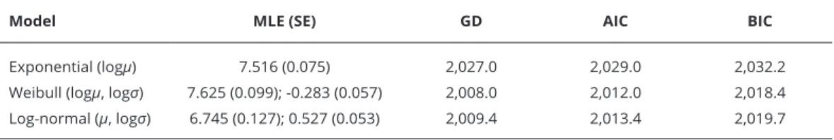
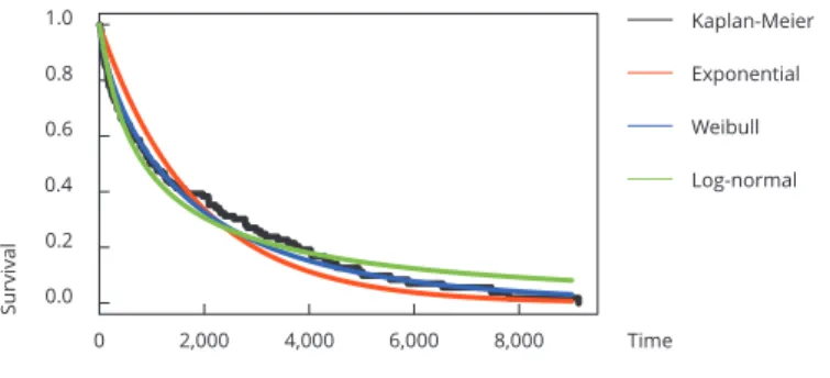
We start the analysis by fitting exponential, Weibull and log-normal models disregarding regression variables. Table 1 shows maximum likelihood estimates (MLEs) and corresponding standard errors (SEs) (in parentheses) of the model parameters and GD, AIC and BIC statistic values for the fitted models. Note that we are considering the structure presented in (1), that is, for positive parameters we use the logarithmic link function μ = exp(β0). We also provide in Figure 2a the plots of estimated
and empirical survival functions. Thus, we conclude that the Weibull distribution provides a good fit to these data.
The TTT plot showed in Figure 2b reveals that the hazard function has decreasing shape. On the other hand, Figure 2c shows that the estimated hazard functions of exponential, Weibull and log-normal models are constant, decreasing and unimodal (increasing and then decreasing), respectively, indicating that the Weibull distribution is appropriate to fit these data.
After selecting the Weibull distribution as the best one to fit these data, we propose a Weibull regression model. Using the steps described in the previous sections to select additive terms for the parameters, we obtain
μ = exp(β01+β11x1+β21x2+β51x5+β61x6+β71x7) (3)
and
σ = exp(β02+β12x1+β52x2+β62x6+β72x7) (4)
For the selected explanatory variables to explain the parameters μ and σ from the Weibull model, we present in Figure 3 the empirical survival curves (Kaplan-Meier) stratified for the categorical variables. In these panels, we can see a great difference between the levels for each variable (gender, kidney transplant indicator, antibodies to hepatitis B and C), agreeing with the selected covariates in the final model.
Table 2 provides estimates, SEs, and p-values obtained from the fitted Weibull model based on GAMLSS. We highlight that all selected parameters are significant at the 10% significance level. Results in Table 2 reveal that the explanatory variables – age at the beginning of treatment, gender, kidney transplant indicator and antibodies to hepatitis B and C – are significant factors to explain the lifetime mean μ of the patients, which is expected from a wide literature that associates these variables as high-risk factors for patients (e.g. Tangri et al. 20 and Fabrizi et al. 21). Moreover, the age at the
beginning of treatment, kidney transplant indicator and antibodies to hepatitis B and C are signifi-cant factors to explain the variability of the shape parameter σ of survival times. A limitation of this study is that few explanatory variables were considered because only those variables were collected by the hospital. Further research, including other variables, may reveal factors not yet discovered in the literature.
Partial effects of the explanatory variables in the mean μ are displayed in Figure 4. From the model for the mean μ, we can see that the older the patient when he starts treatment, the lower is their life-time expectancy (panel (a)). More precisely, for each additional year at the beginning of treatment, the patient’s average lifetime expectancy decreases 0.036 years (Table 2). The lifetime expectancy is lower in female patients (panel (b)) and in patients who have not undergone kidney transplantation
Table 1
Maximum likelihood estimates (MlEs) of the exponential, Weibull, and lognormal distributions, the corresponding standard errors (SEs) and global deviance (gd), akaike information criterion (aiC) and Bayesian information criterion (BiC) statistics.
Model MLE (SE) GD AIC BIC
Figure 2
Estimated and empirical survival functions, total time on test (ttt plot) and estimated hazard rate function of the proposed distributions.
(panel (c)). Moreover, panels (d) and (e) indicate that patients who have antibodies to hepatitis C and B, respectively, have greater lifetime expectancy.
Regarding the shape parameter σ (Figure 5), as we can see in panel (a), the variable age at the begin-ning of treatment has a positive linear relationship with the variability of patients’ lifetime , i.e. the variability of lifetime increases when patients waited to start treatment. Furthermore, according to panels (b)-(d), the variability also increases when the patient has undergone kidney transplantation and when there are antibodies to hepatitis B and/or C. Here, it is clear that the variability of patient’s lifetime must be modelled as well, and not only the mean (as more traditional models such as classical linear regression or generalized linear model usually do), which could mislead us on the selection of false risk factors for kidney failure.
Figure 6 shows some residual plots that can help to verify the adequacy and the assumptions of the chosen fitted model given in (3) and (4). Panel (a) suggests that the normalized quantile residuals have approximately normal distribution. Panel (b) shows that there are few points off the line in the low end of the range. Finally, as we can see in panel (c), the WP also suggests that there is a slightly problem in the lower tail of the distribution of T. The correct would be the fitted cubic model (red curve) to be a line on the X-axis. Nevertheless, the Weibull regression model based on the GAMLSS framework provides a reasonable fit to these data.
Finally, using the results presented in Table 2 we can calculate the average lifetime for each level of the explanatory variable selected in the regression model. Averages are easily obtained using the estimated linear structure:
Figure 3
Empirical survival curves for gender, kidney transplant indicator, antibodies to hepatitis B and antibodies to hepatitis C.
Table 2
Estimates, corresponding standard errors (SEs) and p-values from the itted Weibull generalized additive models for
location, scale and shape (gaMlSS) regression.
Parameter Estimates SE p-value
β01 8.905 0.308 < 0.001
β11 -0.036 0.004 < 0.001
β21 0.444 0.117 < 0.001
β51 0.282 0.144 0.052
β61 0.429 0.125 < 0.001
β71 0.531 0.129 < 0.001
β02 -0.795 0.238 0.001
β12 0.008 0.003 0.027
β52 0.860 0.180 < 0.001
β62 0.756 0.207 < 0.001
β72 0.121 3.885 < 0.001
Note: x
1: age (in years) at the beginning of treatment; x2: gender; x5: kidney transplant indicator; x6: antibodies to
Figure 4
Fitted terms for the mean μ: age (in years) at the beginning of treatment, gender, kidney transplant, antibodies to hepatitis C and antibodies to hepatitis B.
Consider the high-risk group (x1 = maxx1 = 88, x2 = 0, x5 = 0, x6 = 0 and x7 = 0) and the low-risk
group (x1 = minx1 = 17, x2 = 1, x5 = 1, x6 = 1 and x7 = 1). The average of the lifetime for high-risk and
low-risk groups is 310 and 21,568 days, respectively, which correspond to 0.84 and 59 years, respec-tively. The same idea can be used to estimate the average lifetime for any level of explanatory variables.
Concluding remarks
Figure 5
Figure 6
Contributors
T. G. Ramires, L. R. Nakamura, A. J. Righetto, E. M. M. Ortega and G. M. Cordeiro equally contributed for the conception and design of this manuscript.
References
1. Cardozo MT, Vieira IDO, Campanella LDA. Alterações nutricionais em pacientes renais crônicos em programa de hemodiálise. Rev Bras Nutr Clı́n 2006; 21:284-9.
2. Marques AB, Pereira DC, Ribeiro RCHM. Mo-tivos e frequência de internação dos pacientes com IRC em tratamento hemodialı́tico. Arq Bras Ciênc Saúde 2005; 12:67-72.
3. De-Lima JJG, da-Fonseca JA, Godoy AD. Dial-ysis, time and death: comparisons of two con-secutive decades among patients treated at the same Brazilian dialysis center. Braz J Med Biol Res 1999; 32:289-95.
4. Andrade LGM, Gabriel DP, Martin LC, Cruz AP, Balbi AL, Caramori JT, et al. Sobrevida em hemodiálise no hospital das clı́nicas da Facul-dade de Medicina de Botucatu, Unesp: compa-ração entre a primeira e a segunda metades da década de 90. J Bras Nefrol 2005; 27:1-7. 5. Sims RJA, Cassidy MJD, Masud T. The
in-creasing number of older patients with renal disease. BMJ 2003; 327:463-4.
6. Grassman A, Gioberge S, Moeller S, Brown G. ESRD patients in 2004: global overview of pa-tient numbers, treatment modalities and asso-ciated trends. Nephrol Dial Transplant 2005; 20:2587-93.
7. Bommer J. Prevalence and socio-economic as-pects of chronic kidney disease. Nephrol Dial Transplant 2002; 17:8-12.
8. Oliveira MB, Romão JE, Zatz R. End-stage renal disease in Brazil: epidemiology, preven-tion, and treatment. Kidney Int 2005; 68:82-6. 9. Leão JR, Pace FHDL, Chebli JMF. Infecção
pelo vírus da hepatite C em pacientes em he-modiálise: prevalência e fatores de risco. Arq Gastroenterol 2010; 47:28-34.
10. Ferreira RC, Teles AS, Dias MA, Tavares VR, Silva AS, Gomes SA, et al. Hepatitis B virus infection profile in hemodialysis patients in Central Brazil: prevalence, risk factors, and genotypes. Mem Inst Oswaldo Cruz 2006; 101:689-92.
11. Sancho LG, Dain S. Análise de custo-efetivida-de em relação as terapias renais substitutivas: como pensar estudos em relação a essas inter-venções no Brasil. Cad Saúde Pública 2008; 24:1279-90.
12. Rigby RA, Stasinopoulos DM. Generalized ad-ditive models for location, scale and shape. J R Stat Soc Ser C Appl Stat 2005; 54:507-54. 13. Cordeiro GM, Ortega EM, Ramires TG. A new
generalized Weibull family of distributions: mathematical properties and applications. J Stat Distrib Appl 2015; 2:13.
14. Stasinopoulos DM, Rigby RA. Generalized additive models for location, scale and shape (GAMLSS) in R. J Stat Softw 2007; 23:1-46. 15. Ramires TG, Cordeiro GM, Kattan MW, Hens N,
Ortega EMM. Predicting the cure rate of breast cancer using a new regression model with four regression structures. Stat Methods Med Res, 2017; 1-17.
16. Nakamura LR, Rigby RA, Stasinopoulos DM, Leandro RA, Villegas C, Pescim RR. Model-ling location, scale and shape parameters of the Birnbaum-Saunders generalized t distribution. J Data Sci 2017; 2:221-38.
17. Dunn PK, Smyth GK. Randomized quantile re-siduals. J Comput Graph Stat 1996; 5:236-44. 18. van Buuren S, Fredriks M. Worm plot: a
sim-ple diagnostic device for modelling growth reference curves. Stat Med 2001; 20:1259-77. 19. Stasinopoulos MD, Rigby RA, Heller GZ,
Vou-douris V, De Bastiani F. Flexible regression and smoothing: using GAMLSS in R. London: Chapman and Hall/CRC; 2017.
20. Tangri N, Grams ME, Levey AS, Coresh J, Ap-pel LJ, Astor BC, et al. Multinational assess-ment of accuracy of equations for predicting risk of kidney failure: a meta-analysis. JAMA 2016; 315:164-74.
Resumo
A insuficiência renal crônica é um grave proble-ma clínico e de saúde pública no mundo inteiro. Recentemente, apesar de muitas pesquisas já rea-lizadas para identificar os fatores relacionados à evolução dos pacientes renais crônicos, os resul-tados conflitantes entre diversos estudos sugerem a necessidade de pesquisas por região. Portanto, o estudo busca predizer e identificar os fatores as-sociados à evolução dos pacientes com insuficiên-cia renal crônica (IRC) na área metropolitana de Maringá, Estado do Paraná, Brasil, com base nos modelos aditivos generalizados para localização, escala e forma (GAMLSS). Os dados utilizados neste estudo foram coletados no Instituto do Rim de Maringá e incluem 177 pacientes (classificados com IRC, a maioria tratada no Sistema Único de Saúde) inclusos no programa de hemodiálise entre 1978 e 2010. Através dessa abordagem, concluí-mos que em outras regiões, gênero, indicação para transplante renal e anticorpos aos vírus das hepa-tites B e C são fatores significativos que afetam a sobrevivência esperada.
Análise de Sobrevida; Insuficiência Renal; Nefropatias
Resumen
La insuficiencia renal representa un problema médico y de salud pública serio en todo el mundo. Recientemente, pese a los muchos estudios que se han desarrollado para identificar factores relacio-nados con la esperanza de vida de los pacientes con insuficiencia renal, los resultados controvertidos de algunos estudios sugieren que las investigacio-nes deberían realizarse por regioinvestigacio-nes. No obstante, en este trabajo pretendemos predecir e identificar los factores asociados con la esperanza de vida de pacientes con fallo renal crónico (FRC) en el área metropolitana de Maringá, Estado de Para-ná, Brasil, basado en el marco de modelos aditi-vos generalizados para ubicación, escala y forma (GAMLSS por sus siglas en inglés). Los datos usa-dos en este estudio fueron recogiusa-dos del Instituto del riñón de Maringá y comprende a 177 pacien-tes (clasificados con FRC y en su mayoría siendo tratados en el Sistema Único de Salud), inscritos en un programa de hemodiálisis desde 1978 has-ta 2010. Usando este enfoque, concluimos que en otras regiones, género, indicador de trasplante de riñón, anticuerpos a la hepatitis B y anticuerpos a la hepatitis C son factores significativos que afec-tan a la esperanza de vida.
Análisis de Supervivencia; Insuficiencia Renal; Enfermedades Renales
Submitted on 04/May/2017