A Work Project presented as part of the requirements for the Award of a Masters Degree in Economics from the NOVA- School of Business and Economics
Growth Accounting:
How institutions affect Portugal's Growth
Ariane Vaz Dinis (mst 14000432)
A Project carried out on Macroeconomics Applied Policies, under the supervision of:
Growth Accounting: How institutions affect Portugal's
Growth
Ariane Vaz Dinis
June 21, 2013
Abstract
The main objective of this Work Project (WP) is to understand whether institutional quality has been determinant to the increase of Portugal's productivity. This WP provides a sector-wise Growth Accounting exercise and analyzes the Total Factor Productivity (TFP) growth. Sec-ondly, it uses a cross-country approach to understand which institutional indicators influence TFP growth. This WP considers, based on GMM estimation, different models to capture the causality between productivity growth and Institutional Quality. The results obtained reveal a positive relation between TFP growth and Institutional Quality.
Keywords: Growth Accounting, TFP, Institutions, Portugal, Sector
1 Introduction
European integration has provided an ideal context to understand the economic growth and con-vergence process between a group of developed countries, as its survival is dependent on real convergence. European integration focused primarily on the removal of barriers to international competition which should have led to a more competitive economy, flourishing development and innovation. The integration has risen expectations of further market integration, and of institutional and productivity convergence. The European Union defined baseline criteria to optimize the catch-ing up process based on investment in physical capital, human capital, and monetary stabilization; where all member-states had reforms and requirements to meet in order to enter the union. In sum, the expectations of economic integration were defined as differences of factor intensity combined with factor mobility which would lead to a higher efficiency and a higher aggregated income; thus implying a convergence of production levels and income distribution1. However, in light of the
recent European crisis doors have opened to rethink the convergence process and to identify the missing ingredient for real convergence. Portugal entered the EU (originally the European Eco-nomic Community), in 1986, in a very bad shape with serious distortions in the product and factor markets, as well as with an industrial structure in need of modernization. Portugal's external sector was based on traditional consumer goods such as clothing, textile and wood industries; all which were very sensitive to the European Business Cycle2. At the time, a discussion rose about the
gap between real and nominal convergence (Commission, 1997) - economic policy did not seem able to support both types of convergence. Many programs were designed and funds allocated to increase competitiveness and improve production conditions in various sectors.3 However, many
economists advocate that the lack of institutional convergence is the reason behind the low growth. The insufficient real convergence of Portugal towards the EU15 can be solved through structural reforms. However, understanding which structural reforms are necessary or which incentives are needed to create a more competitive economy is the ongoing challenge.
This work project (WP) aims to understand Portugal's evolution throughout this integration 1Islam (2003) argues that many studies have failed to demonstrate that productivity-convergence is associated with
income-convergence.
2Many economists, including Marques-Mendes and da Silva Lopes (1993) argue that the downturn of the growth
rate was due to external factors- balance of payments and deterioration of the terms of trade
3The EU Commission (1997) pointed out the main lines of reform to sustain the convergence process (1)
process. The WP provides a sectoral growth accounting exercise to understand the evolution of sector-wise productivity, and analyses whether institutions are determinant to increase productivity. In spite of the importance of this subject, very little attention has been attributed to institutional quality augmenting productivity. Basically, this WP looks for evidence of the relation:
Institutional Change→Total Factor of Productivity→Economic Growth
This WP used different panel data models, such as the FE and RE, to understand how insti-tutions are related to productivity growth. Concerns regarding reverse causality led to a more compelling approach by using GMM estimation.4
The remainder of this WP is divided into six sections: Section 2 -Literature review concerning all the WP; Section 3- Growth Accounting which is divided into data description and TFP growth calculations; Section 4- Institutional Framework concerning how institutions are integrated into the framework; Section 5- Model specification; Section 6-Results and finally, Section 7- Discussion.
2 Literature review
The Neoclassical growth theory considers the sources of output growth to be the junction of capital and human accumulation with exogenous technological change. However, regarding convergence processes Maddison (1996) defends that growth accounting is a better approach to explain the Eu-ropean catching-up process to US productivity levels, as it drops the constant elasticity assumption inherited from the neoclassical framework.
The growth accounting literature from Solow (1957) to Hall and Jones (1999) reveals that the best measure of productivity is Total Factor Productivity (TFP). Yet, the TFP or Solow resid-ual's content or captured factors has not yet been defined with consensus among economists. Abramovitz and David (1996) define the residuals as "the measure of our ignorance" since it is an important explanatory growth factor, nonetheless disagreement persists due to the lack of data availability and diversity of methodologies. A common consensus is that TFP is the economy's capacity of converting inputs into outputs. There are two types of methods to calculate Total Factor Productivity: one deterministic and the other econometric. Growth accounting lies in the deter-ministic class as the residuals are "calculated"; while growth regressions are based on econometric 4Results are presented using the estimator xtabond2 in Stata created by Roodman (2006) as tool to control for
methods thus residuals are "estimated" through models.5 The main advantage of the growth
ac-counting approach is that TFP is not an estimated residual obtained through a calibration exercise. The TFP measure can use a traditional non-frontier methodology (Solow, 1957) which follows an assumption of fully efficient production implicating that the observed output equals to potential level. The Frontier models allow for inefficiencies6- output is not assumed to equalize the frontier
output. In this WP, we will use growth accounting with maximizing profit and constant returns to scale using a non-frontier methodology.
In the growth accounting methodological approach, Islam (2003) considers three main ap-proaches: (1) "time-series growth accounting" (developed by Jorgenson to calculate productivity growth rates7); (2) "a panel regression approach" (used to estimate productivity levels by Islam
(2003)) and (3) "a cross-section growth accounting approach" (considered in Hall and Jones (1999) to compute levels of productivity8).
Economic growth has been in the limelight throughout centuries as the driver of higher wel-fare. Explaining wealth differences has been the foundation for the quest to find the sources and determinants that create economic growth. Hence, a vast literature regarding the determinants of economic growth,9 where we emphasize capital accumulation, capital labor, governance, and
in-stitutional framework, has emerged. Ultimately, growth is driven by individual behavior of house-holds, firms and research institutions whose incentives are provided by formal and informal rules. These decisions depend largely on the structure provided by the government regarding property rights, capital investments, labor utilization, capital labor, capital deepening, innovative protection and infrastructure. Institutions also play an important role in this context. North (1990) defines institutions as
"The rules of the game in society or, more formally, are the humanly devised con-straints that shape human interaction. In consequence they structure incentives in human exchange, whether political, social, or economic."
Good institutions can avoid losses due to corruption, destruction of capital, legal procedures, en-5According to Del Gatto et al. (2011) productivity measures are organized with these criteria.
6Data Envelope Analysis is a nonparametric frontier method that decomposes output growth into technology change,
quality improvement, real cost savings and efficiency change.
7This approach was followed by (Timmer et al., 2007) and we have also used it. More details are available below. 8Hall and Jones (1999) compute the productivity levels, although it allows the capital share to vary across countries,
they are restrained by the assumption of equal rate of return to capital.
9A summarized list may be found in Wacziarg (2002). Durlauf et al. (2005) present an extensive literature review
forcement of contracts and macroeconomic stability. The public sector has a prominent role to provide a market structure to facilitate the absorption of technology and the development of com-petitive markets. Consequently, institutions have a direct influence on household and business decisions which ultimately influence total factor productivity. The global economy is in constant evolution forcing institutions also to evolve to accommodate changes endogenously. Despite, this evolution, institutional reforms are used to re-order priorities and maintain competitiveness. Nev-ertheless, institutional quality is hard to measure, and still we only have very incomplete proxies available10.
The relation between institutions and growth has been vastly studied. Many papers11resort
to cross-country empirical studies to understand growth differences and empirically test whether institutions are the main determinants. North's institutional framework could be integrated with the Solow growth model; Abramovitz and David (1996) highlight that the absorption of technology is constraint by "social capabilities". The rate of technical progress and efficiency is affected by institutional quality.
Hall and Jones (1999) are responsible for the turning point of considering the effect of social infrastructures as drivers of productivity12in a cross-country study, finding that the social structure
has significant effects on long run economic performance. However, looking deeply into institu-tions, both formal and informal institutions are prominent in explaining incentives that could lead to an increase in productivity.
Summing-up, this WP follows the "New Growth Theory" which goes beyond neoclassical as-sumptions of factor accumulation, whereas the rate of technological progress is driven by internal forces to the economic system. Aghion and Howitt (1990) underlines that sustained long-term growth is achieved through a boost in technological change driven by a more efficient use of re-sources. Competitive firms have incentives given by policies to maintain a competitive edge by constantly innovating; altogether R&D efforts create a higher efficiency leading to technological progress. Thus, there is also a scale effect to be considered that influences the growth rate of technological progress. The New Growth Theory was empirically tested by considering the Total Factor Productivity as a proxy of technological change capturing efficiency gains; and to control 10The EBRD is monitoring the EU new-member convergence process to create better institutional quality indicators.
11Milestone references, such as Acemoglu et al. (2000), Knack and Keefer (1995), Dollar (1992) and Rodrik (2000)
use proxies for institution (such as property right, risk of expropriation, contract enforceability, political systems, etc.) and use instrumental variables to capture institutional effects (settler's mortality, language, colonial origins, etc).
for scale-effects we use country-industry level R&D stocks.
There are many studies regarding Portugal's productivity evolution. Lains (2003) has done an historical analysis of Portugal's productivity based on a econometric model considering structural changes in the industrial sector. Amador and Coimbra (2007) consider a stochastic frontier exer-cise using as baseline Greece, Ireland and Spain to understand what sources of growth are at larger distance from the efficiency frontier. There are also many reports with a policy driven charac-ter regarding convergence to the EU with illustrative TFP growth comparison. The IMF (2013) compares aggregate TFP growth in the US and EU15 concluding that there is an urgent need of technological improvement. The European Commission produces many reports emphasizing the catch-up and growth of member states. All these papers, in general terms, suggest structural re-forms to improve institutional quality. Tavares (2004) addresses the question of which of the struc-tural reforms actually affects growth, using different institutional indicators to understand which are more correlated with the growth of the country. This paper shows compelling evidence that institutional indicators are very correlated with growth. However, the question of whether institu-tional quality drives total factor productivity growth remains unanswered. Hence, is instituinstitu-tional quality the key to growth in a context of convergence?
3 Growth Accounting
The growth accounting exercise is a diagnostic tool that helps understand the economy's produc-tivity throughout time. Aggregate growth accounting rules out the sectoral composition of output, following an assumption of uniform technological progress. However, differences in aggregate TFP may be explained by sectoral specialization, which would imply different policy implica-tions. On the one hand, if productivity differences are explained by the sectoral composition, than policies should be directed towards factor mobility across sectors; on the other hand, if however this is not the case, barriers to productivity are explained through technology adoption. A relevant relationship between aggregate and industry level TFP is that the aggregate measures consider one sector that produces all GDP, whereas all intermediate goods cancel out.13 An increase in
sector-wise productivity occurs either due to improved efficiency gains at the firm level or due to a shift of production towards more efficient establishments (Schreyer, 2001). The effects of policies and 13This raises difficulties when deriving the aggregate to disaggregate output (or TFP) or vice-verse. Hulten (2009)
regulation or technology change have a direct impact on relative productivity leading to relative price changes and changes in the elasticity of substitutions.
3.1 Theoretical Background
The growth accounting industry level framework applied in this WP follows the time-series panel methodology presented in the Schreyer (2001) and Timmer et al. (2007). The production function for each industry given asYj,t=fj(Kj,t, Lj,t, Xj,t), is composed by the industry gross production
output (Y), labor composition (L), index capital services flow (K), index intermediate inputs (X) and technology (A). Considering the production function as a function of time, output has a direct change over time due to impact of changes of capital, labor and intermediate goods over time. Hence, considering the production function over time t, we have that
dY dt = ∂Y ∂K dK dt + ∂Y ∂L dL dt + ∂Y ∂X dX dt + ∂F
∂t . (1)
Regarding the terms of this equation, we have that∂Y ∂K
dK
dt is the capital effect on output, ∂Y ∂L
dL dt
is the labor effect on output and finally,∂Y ∂X
dX
dt is the intermediate input effect. The last term, ∂F
∂t,
is the direct effect of time on output, also called productivity or technology (At). By dividing both
parts of equation (1) byY, we may re-write it as a function of output growth, i.e.,
. Y Y = ∂F ∂t Y + ∂Y ∂K K Y . K K + ∂Y ∂L L Y . L L + ∂Y ∂X X Y . X
X, (2)
which can further be represented as,
. Y Y = ∂F ∂t Y + MPK APK . K K + MPL APL . L L + MPX APX . X X (3) where . Y
Y is the growth rate of output and all other inputs follow same convention. Moreover,
MPK refers to Marginal Productivity of Capital (∂Y
∂K), APK to the Average Product of Capital ( Y K),
MPL is the Marginal Productivity of Labor (∂Y
∂L) and APL the Average Product of Labor ( Y L).
The intermediate product follows the same convention. Furthermore, assuming constant returns to scale, capital intensity is given byαKt = MPKAPK, labor intensity byαLt = MPLAPL and the intermediate
product effect isαXt = MPXAPX.
measure the continuous growth rate of TFP (TPF.
TPF), generally the average value of TPF=△lnTPFt
is considered. Moreover, under assumptions of competitive factor markets and full input utiliza-tion; and considering that firms are price-takers, it follows that,
αKt = MPK
APK =
∂Y ∂K Y K
= RtKt
PtYt
, (4)
αLt = MPL
APL =
∂Y ∂L Y L
= WtLt
PtYt
(5)
and
αXt = MPX
APX =
∂Y ∂X
Y X
= P
X t Xt
PtYt
. (6)
Summing-up, considering equation (2) for each sector, we have that:
△lnYjt =αX△lnXjt+αK△lnKjt+αL△lnLjt+△lnTPFYjt (7)
whereαXt +αKt +αLt = 1 and the technical changeAjt is measured by total factor
produc-tivity (△lnTPFYjt). A crucial assumption is that marginal revenues are equal to marginal costs,
so a weighting procedure is sufficient to ensure that the input indices reflect all the components weighted by their influence on productivity. The aggregation of Output, Labor and Capital use a Tornqvist quantity index14.
3.2 Data
Following the literature, the database used is theEUKLEMS Growth and Productivity Accounts
(EU KLEMS) Revised152008 as a resource of input and output series provided independently of
any econometric method.
Portugal's productivity is assessed at higher depth, using as a baseline comparison average EU low (Portugal, Greece, Italy, Spain and Ireland), average EU high (Germany, France, Netherlands, Belgium, and others), Spain and Germany. We are considering the evolution of productivity in Total Industries (TOT); Agriculture, Hunting, Forestry and Fishing (AtB); Total Manufacturing
14Following the methodologies in Timmer et al. (2007), O'Mahony and Timmer (2009) and Schreyer (2001). Further
specifications may be found in Section 9.1 of the Appendix
15There are a few other data-sets in WIOD or GGDC, but none were as complete and homogeneously corrected for
(D); Finance, Insurance, Real estate and Business sector (JtK); Mining and Quarrying (C); Elec-tricity, Gas and Water supply (E); Construction (F) and Wholesale and Retail Trade (G). Data is not available for all time periods, so our analysis only considers a sample from 1970 to 2005.
3.2.1 Output
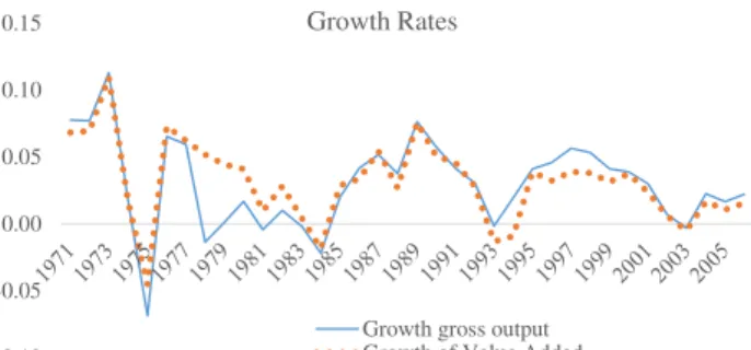
We consider two measures of output- Value Added (VA) and Gross Output (GO). The Value Added is the production each sector provides without including purchases of intermediate goods. While the gross output is the total value of the sales including the three inputs16. Figure 1 illustrates how
the value added growth resembles gross output growth rates.
-0.10 -0.05 0.00 0.05 0.10
0.15 Growth Rates
Growth gross output Growth of Value Added
Figure 1: Growth rate of Value Added and Growth rate Gross Output
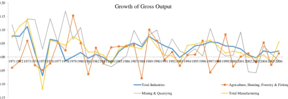
The output of growth rates are sector wise distinct displaying very significant changes within each specific sector. A higher economic integration would lead to higher factor mobility across countries following a distribution of fac-tors according to the factor intensities of each sector. Sectors with a higher relative income of factor within the economy would attract factors
needed, leading to an equalization of factor income - factor intensity equalization. Thus, sectors that are more efficient would be able to grow at a faster rate leading to higher production levels.17
Despite the theoretical reasoning, factor mobility may react very slowly to market driven incen-tives. A country with rigid market conditions can be forced to enter a situation of disproportional production levels due to inefficiency of factor allocation, which creates a gap between efficient and inefficient sectors. However, in a context of economic integration, an even higher mobility between countries would be expected, as a union should converge to the same factor income in all regions. Factor abundance or scarcity are also included in the factor income variation, since these influence the factor-price component. Studying distinctively by sectors should allow for a more profound analysis to understand which sectors have flourished and which have retracted with the integration. An interesting point would also be to consider whether factor mobility across sectors was synchronized with the relative factor income across sectors.
-0.15 -0.10 -0.05 0.00 0.05 0.10 0.15 0.20
1971 1972 19731974 19751976 1977 19781979 19801981 19821983 1984 19851986 19871988 1989 1990 1991 19921993 19941995 1996 19971998 19992000 20012002 2003 20042005 2006 Growth of Gross Output
Total Industries Agriculture, Hunting, Forestry & Fishing Mining & Quarrying Total Manufacturing
Figure 2: Value added growth rate and gross output growth rate by sector.
As expected, the overall production level growth of output should be increasing considering that there is free factor mobility, and that an increase in capital inflows contribute to the effect.
3.2.2 Intermediate goods
-0.15 -0.1 -0.05 0 0.05 0.1 0.15 0.2
Intermediate good
Growth of II_QI Decompose Growth II_QI
Figure 3: Growth rate of intermediate goods: (a) Aggregated intermediate goods; (b) Decomposed aggregated intermediate goods composed by en-ergy, services and material.
The database provides an aggregated index of the intermediate goods and of the inputs de-composed into energy, services and material. However, data availability of the decomposed inputs has a smaller time period than the one being considered. Using a Tornqvist index, us-ing as weights the compensation of each inter-mediate index, we calculated an aggregated in-dex. Figure 3 depicts the growth rate of both indices.
3.2.3 Labor
Portugal has information regarding worked hours and number of labor engaged. When we analyze the growth rate of both variables, we conclude that both have very similar pattern.18 In this case,
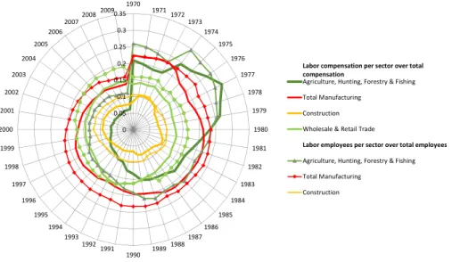
we use total hours worked by persons engaged as labor input. As mentioned above, institutional quality has a direct influence on incentives of labor opportunities. Figure 4 illustrates that the employment share per sector is not evolving according to market signals of higher compensation. Ideally, sectors with higher labor compensation should attract more individuals. However, the share of workers in each sector seems quite stagnated. The mining and quarrying sector, which is
not represented, is quite troublesome as it has a significant amount of workers, but with very low labor compensation. 0 0.05 0.1 0.15 0.2 0.25 0.3 0.35 1970 1971 1972 1973 1974 1975 1976 1977 1978 1979 1980 1981 1982 1983 1984 1985 1986 1987 1988 1989 1990 1991 1992 1993 1994 1995 1996 1997 1998 1999 2000 2001 2002 2003 2004 2005 2006 2007 20082009
Labor compensation per sector over total compensation
Agriculture, Hunting, Forestry & Fishing Total Manufacturing
Construction
Wholesale & Retail Trade
Labor employees per sector over total employees
Agriculture, Hunting, Forestry & Fishing Total Manufacturing
Construction
Figure 4: Relation between labor compensation and employment share in each sector.
The skill composition throughout the sectors is also important to determine labor productiv-ity within each sector. Low skill engaged personnel will induce slower labor movement towards higher skilled-demand sectors. Unfortunately, labor decomposition is only available for the period 1997-200519. Due to the unavailability of data, two different measures of TFP considering both
labor composition and hours worked will be considered.
3.2.4 Capital
The capital input index is composed of an aggregation of assets from land, infrastructure to com-puters. However, not much data is available in the KLEMS database, so input is measured by the ICT and Non-ICT capital. There is lack of detailed sector-wise information regarding capital. The capital index does not account for changes in the usage of land or differences in inventories. However, Timmer et al. (2007) describe how the capital index was set-up, the method of applying depreciation rates to different assets and the treatment of negative capital. The approach used to calculate capital compensation is not based on the exogenous cost of capital information, but rather on differentiating the value added into labor compensation and capital compensation. This process allows for an heterogeneous weighted stock of assets to be included in the index.
0 0.05 0.1 0.15 0.2 0.25
Share of Capital EU high Share of Capital EU low Share of Capital Pt Share of Capital ESP Share of Capital GER Share of Capital FRA
(a) The share of capital as the ratio of capital compensation and current gross output.
0 0.05 0.1 0.15 0.2 0.25 0.3 0.35 0.4
Share of Labor EU high Share of Labor EU low Share of Labor Pt Share of Labor ESP Share of Labor GER Share of Labor FRA
(b) The share of labor calculated as the ratio of labor compensation and current gross output.
Figure 5: The shares used to calculate weights of each factor in the Growth Accounting exercise.
to capital-poor countries leading to expectations of institutional and productivity integration. De-spite, the theoretical reasoning, this leap could only be fostered if government authorities evolved institutions towards further integration. However, looking at Figure 12, we observe that capital based on information processing and technology had the highest advance and growth despite the fall in capital growth after 1999.
Hence, the evolution of capital and labor shares will shed more light towards the role of Capital and Labor input. Figure 5b follows the reasoning that within economic integration, expectations rose labor compensation to the level of average high income EU, despite an unreal market incentive. While capital compensation Figure 5a, which was in high supply is lower than the designated comparisons. Growth accounting uses these shares as the weights of the contribution of each component.
3.3 Total Factor Productivity
Taking all components measured earlier, Table 5 provides an average per year contribution, while Figure 13 illustrates the contribution of each factor to the TFP growth rate. As can be observed, TFP growth follows a very similar path as the output growth rate. The contribution of labor seems to be the most volatile of all components. TFP is measured as the ratio of volume of output to input. This productivity ratio has embedded many characteristics20 that cause change, namely
technological change, technical efficiency, real cost of savings and living standards. Technological change is the innovative process to transform resources into output shifting the frontier of potential production; including innovative products or scientific evolution. Technical efficiency refers to
efficiency gains due to re-organization towards "best practices" at an individual level or concerning shifts of production at an industrial level to more efficient establishments. Real cost savings is a residual that captures all other factors not mentioned above, such as learning-by-doing or social benefits gained in certain sectors, etc.
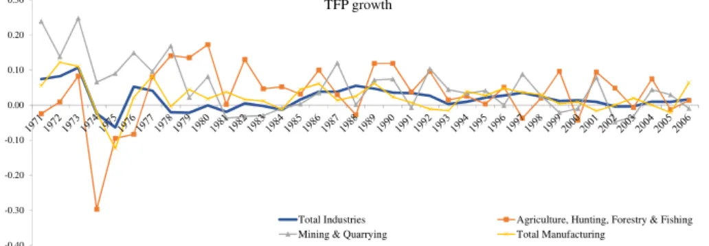
Total Factor Productivity is very different according to the industry considered. We cannot rule out the possibility that some of the variation results from measurement errors. Below, in Figures 6 and 10, we present the differences in growth considering different levels of decomposition.
-0.40 -0.30 -0.20 -0.10 0.00 0.10 0.20
0.30 TFP growth
Total Industries Agriculture, Hunting, Forestry & Fishing Mining & Quarrying Total Manufacturing
Figure 6: Total Factor Productivity growth rates using only aggregated sector-wise indices
However, due to data availability the present TFP growth does not include the desegregated labor and intermediate good decomposition presented in the formulas in the Appendix. When we allow for different decompositions the growth of TFP takes a very similar path (see Appendix Figure 1121).
Altogether, these differences bring forth a more skeptic look towards the calculation of growth of TFP. Looking further to the differences in growth of TFP in each sector compared to an aver-age of EU high, EU low and baseline countries (Figure 7) hinges on the fact that they are good indicators of productivity22.
‐0.05 0 0.05 0.1 0.15 0.2
0.25 TFP_TOT EU high
TFP_TOT EU low
TFP_TOT PT
TFP_TOT ESP
TFP_TOT GER TFP_TOT FRA
Figure 7: Total Factor Productivity growth aggregated TFP growth in comparison with EU 15
21The KLEMS database methodology corrected all variables to homogenize series.
The convergence of EU countries' productivity growth is still under discussion. Stylized facts are that lower productivity countries will have higher productivity growth rates, while higher pro-ductivity countries will have low growth rates23. In respects to the convergence process in a market
integrated setting, we will assume that productivity growth among the same sectors across coun-tries will converge to the same growth rate, considering that there is a high diffusion of technology and free factor mobility among member-states.
4 Institutional Framework
In this WP, we consider only formal institutions to understand the casual relation with produc-tivity24. Following a similar framework as Hall and Jones (1999), we consider the quantitative
measure of institutional quality (IQ) as a determinant of productivity (TFP) through a structural model, i.e.,
logTFPit=α+β1IQit+ǫit (8)
IQit =γ+δlogTFPit+θXit+ηit (9)
where, IQitis institutional quality, TFP is the TFP growth rate25. This specification is
parsi-monious since it ignores many other factors that contribute to productivity, focusing mainly on the role played by institutions. However, given that there is no perfect institutional quality measure, the proxy for institutions can lead to significant measurement errors IQ = ¯IQ+v; where IQ is
the proxy,IQ is the true value and¯ vis the measurement error. This error creates a downward bias
of the OLS estimator. As empirical evidence has demonstrated (8) has an endogeneity problem between institutions and productivity.
Aron (2000) highlights many problems concerning causality between growth and institutions: (a) Reverse Causality: higher growth creates better institutions and better institutions create opti-mal conditions for growth. (b) Endogeneity: where institutional quality is not constant or
exoge-23Many papers are focusing on the question of convergence within the EU. No consensus has yet been reached, as
only predictive models were constructed.
24Time constraints limit us of looking further into the gap between informal and formal institutions
25Hall and Jones (1999) emphasize the importance of TFP levels rather than growth rates. Where level analyses are
nous. It may be affected by political instability, climate shocks, trade or even austerity programs. (c) Institutions: there is no variable for institutions, considering that it represents a state that de-pends on many variables. Most institutional criteria are ordinal indices ranked across countries, meaning they do not quantify institutional differences, but consider a relative rank. (d) Omitted variables: is a constant concern regarding regressions; especially reverse causation combined with omitted variables were there is no assurance for the unexplained growth variance.
4.1 Institutional Indicators
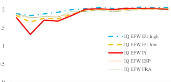
There are two types of institutions: (a) Formal institutions which are an endogenous bureaucratic evolution in terms of laws, economic and political level; (b) Informal institutions are exogenous and cultural based rules and incentives. Formal institutions, in general, are based on an aggregation of hard variables; however, many indicators also aggregate a soft component. Meanwhile, informal institutions are generally based on soft indicators created through surveys data and perceptions. Generally, it is believed that institutional quality indicators have an inherit biased construction, since the weights and variables included in the indicators are left at the researchers discretion.
0 0.5 1 1.5 2 2.5
1970 1975 1980 1985 1990 1995 2000 2001 2002 2003 2004 2005
IQ EFW EU high
IQ EFW EU low
IQ EFW Pt
IQ EFW ESP
IQ EFW FRA
Figure 8: Institutional quality indicator based on the Economic Freedom World- Fraser Institute. Institutions are very hard to measure, as can be
inferred from North (1990). Alonso and Garci-martín (2013) indicate that a good institutional quality indicator has to incorporate at least four properties: 1) static efficiency - ability to en-hance efficient equilibrium by a technological frontier; 2) credibility- generate a framework capable of enforcing incentives and modulate
the many variables, each component and sub-component is scaled from 0 to 10 and averaged into aggregate form. This indicator is only available in intervals of 5 years during the period of 1970 to 1995, however it is available yearly in the periods afterwards. In Figure 8 there is distinctly a process of institutional catch up as is expected with economic integration, however the institutional convergence is dependent on the country's characteristics. The IQ_EFW is a hard indicator based on statistical variables to measure formal institutions.
5 Model Specification
5.1 Cross-Country Model Specifications
In order to understand how institutions affect the TFP industry-level, we use an unbalanced database of 23 countries (i=1,...,23) for 6 aggregated sectors (j=1,...,6) for the years from 1970 to 2005 (T < 35). A panel-data approach requires more attention than a cross-section study, as the standard errors of the panel estimator have to be adjusted to dependency between time periods. Wooldridge (2002) highlights that in comparison to cross-section, panel data provides more possibilities of addressing the presence of omitted variablesCov(x, c)6= 026.
A cross-country panel data approach opens a wide range of possibilities of different models based on the equation below:
△lnTFPi,j,t =αj,t+αi,t+β1RDi,j,t+β2IQi,t+ǫi,j,t (10)
where R&D stock (RD) is a control for sector scale effect;αj,t corresponds to industry-specific
effects; andαi,t is the country effect given by the time-varying institutional indicator. The
insti-tutional indicators are invariant for all sectors. Hence, the productivity growth may vary across sectors but are controlled by country institutional effects. Two different approaches can be taken into consideration resulting into different implications as shown in (11) and (12) below. Thus, the first is,
△lnTFPit=αi+β1IQit+α1RD+ǫit. (11)
26In the cross-section we are limited to (1) appropriate proxy; (2) 2SLS method with instrumental variables for x and
Regression (11) considers the TFP growth rate of each sector individually. Considering the low number of countries, assumptions regarding the nature of the time series dependence are necessary as to obtain an efficient estimator. The analysis will have a panel of approximated Countries (N) x Time (T) observations. The FE models consider the individual country effects and can also control for the the time effects. The second regression is,
△lnTFPjit=αi+β1IQit+α1RD+ǫjit (12)
This regression considers the TFP growth rates of all sectors controlled by sectors, following a panel with more observations for the time period. We will control for the significance of country effects, sector effects as well as time-effects; as to understand which are the most interesting. This panel will have many observations as i=1,...,29 and j=1,...,6, so we obtain 174 observations for each time period. Fixed effects and Random effects estimators will be considered to obtain adequate coefficient estimates.
Nevertheless, we can see from equation (10) that the assumption of the idiosyncratic error term
ǫi,j,tbeing i.i.d is unlikely to hold. Additionally, the panel data model has also to be corrected for
autocorrelation and heteroskedacity as it is highly likely. Besides, the model is a structural equation with a problem of reverse causality, where feedback effects are a major concern.
Arellano and Bover (1995) suggest that a system GMM estimator is highly advantageous in such cases, and is very efficient in large country/sector and short time dimensions. System GMM uses lagged regressors as instruments, thus endogenous variables are determined directly from past values ensuring that these are uncorrelated with the error term. Specifically to the system GMM estimator, a dynamic panel data model is considered, leading to the regression,
△lnTFPjit=αi+δ△lnTFPj,i,t−1+β1IQit+α1RD+ǫjit (13)
6 Results
Wooldridge (2002) discusses the advantages of a panel approach in comparison to cross-section studies to deal with endogenous components in the regressions. In this case, the panel offers attrac-tive solutions to capture the endogenous component of institutional quality, by capturing invariant effects through time. Fixed and Random effects models give appropriate tools to hold fixed coun-try specific idiosyncratic effects or to consider randomness among individuals - handling omitted variables. As discussed before, regressions encounter many problems derived from time-invariant country characteristics such as geography, culture and demographics that can be highly correlated with the explanatory variables. These arbitrarily distributed fixed effects remonstrate cross-section, as these ignore the effects, while in panel the variation overtime allows for identification of the pa-rameters. This WP gathers intuition referring to different controls for fixed effects, varying from controls across individual countries, as well, as controls for effects specific to sectors or using ran-dom controls. Despite these advantages, the main problem lies on data availability through long enough panels. Unbalanced panels can originate inconsistent estimators. This WP used an unbal-anced panel- however, since there is a clear selection of countries towards high-income countries with very similar characteristics; we would consider these effects mitigated. Besides, the unbal-anced panel is rooted from unavailability of continuous long period institutional indicators. This WP gives a higher emphasizes to the linked chain overall score of World Economic Freedom. The index has been corrected as a linked chain through a larger time span than the other institutional in-dicators that were found. The indicator has as well been corrected to the fact that more components were added through time to create a more accurate institutional indicator.
panel bias, anyhow fixed effects in the disturbance term create endogeneity not correctable through dummies.
Altering the estimation model to equation 12 and restructuring the panel setting, to a panel with more observations as i=1,...,29 and j=1,...,6, so as to obtain 174 observations for each time period (t=1,...,34) discounting the unavailable 20 years with gaps in the institutional indicator. This constructions allows a further clustering of standard errors to sector characteristics; assuming sectors productivity has a constant variance across countries. In this case, we can opt to control for country specific fixed effects; whereas if sector effects and individual effects are correlated than the FE model makes incorrect inferences regarding the relation. Also, the RE assumes idiosyncratic effects to be uncorrelated with the predictor which allows effects to affect the error. Results for this model are basically, very similar to the results presented above.
Going back to the structural equation of productivity and institutional quality in section 4, the challenging problem to solve is the reverse causality of the institutional quality. This issue is usu-ally solved through a fixed effects estimator corrected through two-stage least squares instrumental variable estimation. In spite of the attempts, no appropriate instrumental variables are available to differentiate between country specificity considering these very similar countries. We considered literacy, openness and other political institutional component as possibilities. On the one hand, we considered using these as time-invariant which would limit the power of the time-series approach; on the other hand, if the variables were time-varying alongside the productivity growth, there would be high correlation leading to a discussion of the weakness of the instrument. Reason why we use the Arellano and Bover (1995) system GMM estimator, which is built from stacking the data set in levels and in differences. The system GMM combines two equations: a first-differences equation with level lagged instruments and a level equation with lagged differences as instruments. The GMM assumes that past changes are uncorrelated with current errors in levels, and also uncor-related with fixed effects. The system GMM is a dynamic panel estimator - estimating equation (13).
GMM allows for endogeneity, measurement errors and omitted variables, as well as, fixed effects and autocorrelation between coefficients.
We use the xtabond2 command in Stata, developed by Roodman (2006), as it has many cor-rections essential to the characteristics of this data-set. First-off, the estimator provides a two-step estimation of the covariance matrix, adjusting for heteroskedasticity and autocorrelation through robust and clustered standard errors. The use of instrumental variables results into a finite-sample corrected two-step covariance matrix. Secondly, it offers an option of transformation "forward orthogonal deviations", which allows for missing values, whereas the instruments (or deeper lags) are orthogonal to the error. Finally, the estimator provides distinguishable control for different effects, not only on the regressor, but also controls for the instrumental variables; the estimator allows exogenous and endogenous controls on either subset of equation. Regarding, the model fit, we considered a two-step estimation with orthogonality deviations and sector-wise standard errors clustering.
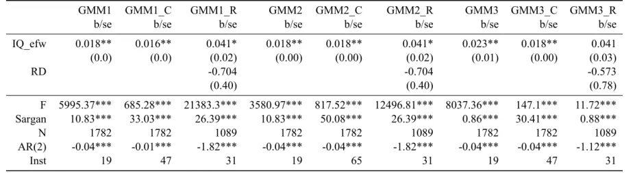
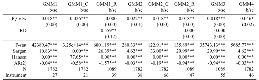
Our results using the system GMM estimator were not as brilliant as would be expected; see Tables 6 and 7. The coefficients vary from 0.017 to 0.04 considering as an exogenous Instrumen-tal variable (IV) the years dummy, meaning that a 1% increase in the in. Undoubtedly, Table 7 illustrates the whole issue of too many controls and a small sample size problem.
The assumption of uncorrelated differences instruments and the variables used in levels with unobserved country effects, is crucial in a panel fixed effects model. Assumptions regarding the initial state or control effects play an important role to delineate the transitional path. We include all variables uncorrelated with fixed effects only in the level equation.
Nevertheless, the coefficients that are statistically significant display a positive relation with the productivity growth. In spite of inclination to use the R&D stock as to control the scale effect of each country, there seems to be a high negative correlation between the institutional quality and R&D stock variablecorr(TFP_sector, R&D) = −0.4680. Whenever, one of the coefficients is
positive and significant, the other is negative and insignificant. Only in one of the specifications, with no controls, and only year and sector IV, were both coefficients positive, but statistically insignificant. Nevertheless, the growth of TFP is sufficiently informative of the country effects and scale effects, to consider the model without the R&D.
identify model fitting problems that are grounded in the system GMM characteristic trade-off quest27, i.e., include deeper lags for a better fit at the cost of inefficiency obtained from a
re-duced sample. Here we suspect that the model has "symptoms of instrument proliferation" which would lead to misleading apparently valid results. Roodman (2009) emphasized that these are originated from over-fitting endogenous variables and/or imprecise optimal weighting matrix. The over-fitting problem is not as relevant in this case, because as observed, in the robustness test, by collapsing the instruments into blocks, we remain with similar coefficients and smaller standard errors. With some exceptions, where the controls significantly reduce the sample, the coefficient of the collapsed estimation is very similar. We did not present the dummy coefficients, as most are dropped due to collinearity or have omitted results. As highlighted in Roodman (2009) " the bias with endogenous regressors is far worse" compared to over-fitting the endogenous variable bias. Giving a stronger power to the estimation coefficients. The second issue raised, regarding the estimates of the optimal weighting matrix, mainly bias the statistical tests, however, do not affect the parameter estimates consistency. This problem regards the distance the estimator is from the asymptotically efficient estimator due to the high number of instrumental variables. In this case, the small T periods available, after missing data count, would incline to consider that the problem faced concerns the optimal weighting matrix.
These results would seem more promising if our institutional indicator had stronger statistical power. As can be seen from the cross-correlations, Table 2, the relation is not strong. Besides, the indicators' missing gaps in the initial periods make inference weaker. The overall construction of the Institutional Quality indicator, also limits the power of this cross-country studies. It is important to question the variability of the Institutional Quality indicator, when we assume such a selected high-income group of countries. The scale of the indicator is from 0 to 10; our country sample has a minimum of 3.6 and maximum of 8.65; the mean is 7 while the variation 0.81.
However, using other available institutional indicators, has not generated more convincing re-sults; see Table 8. In spite of statistically significant coefficients, the WGI indicator had a negative relation with productivity, while IEF has a positive but very small coefficient. As a robustness check, we also considered the five major components of the Economic Freedom Indicator inde-pendently to understand the causality between institutions 10. However, more complex estimations 27To avoid this problem, literature uses the first-difference GMM estimator, however, this estimators eliminates the
can not be considered since, the sample size is too small to hold for more controls. As mentioned above, we also aimed to understand how each sector's productivity reacts to different institutional indicator, nevertheless, the unbalanced panel characteristics drops the sector dummies. Further-more, different panel structures did not facilitate the process of studying sector specific productivity growth.
7 Discussion and Conclusion
Frequently the literature resorts to explaining growth differences through productivity divergence. But, as emphasized by Islam (2003), productivity growth rates and convergence are still under the microscope, and results from different growth accounting methodologies lead to very different econometric outputs. Many factors such as, e.g., scale effects, externalities, technological diffu-sion, culture, formal and informal institutions, or even the economic situations, contribute to the productivity growth of a country. As emphasized by Hulten (2009)'s critique, new innovations or higher technology goes beyond a shift in the production function. Methods that use microe-conomic based technological assumptions to estimate the parameters eliminate scale effects and externalities ((Hall and Jones, 1999)). Extending Hulten (2009) discussion, he argues that there is a trade-off in choosing a growth accounting methodology; the productivity measure can incorporate more effects using non-parametric methods, but at the cost of accuracy.
link between the incentives to accumulate capital and to innovate with institutional quality. These effects go beyond the scope of this WP, but we do consider that Institutional Quality is endogenous to both effects.28
Additionally, the growth rate of productivity eliminates the noise and appeases data volatility. Especially, since we are interested in the convergence behavior of productivity; the productivity levels would not be a stationary series, leading to explosive behaviors. By using the growth of pro-ductivity, we may further infer about technological differences across sectors and analyze different adjustment paths.
A discussion regarding the efficiency of a system GMM estimator applied to this model and database has already been provided in the Results section. To accentuate the advantages brought by the system GMM to estimate the convergence across sectors, we highlight the assumption that the estimator requires a mean stationarity condition for each individual; whereby in conjunction with persistent TFP growth is ideal to capture TFP growth rates with different initial starting points (regardless of whether it is satisfied in the model).29 The system GMM estimator is valid as long
as such a steady state is reached in the period at hand. Additional covariates establish the long run means of TFP growth conditional on the covariates. Further on, we will always consider the evidence and results of the GMM estimator.
This WP assumes that each sector has its own specific effects that will converge among coun-tries, which are more relevant than a country effect cluster; reason why we cluster sector-wise30.
Basically, we assume a technology diffusion across sectors implying that these should converge to the same productivity growth rate. A very criticized point raised in aggregate studies, is that Output and TFP growth, rules out sector decomposition; as by assumption they are considered as identical within productivity. This study should have shed light on the differences of TFP growth by sector, understanding which are more vulnerable to institutional change. For example, Infor-mation and Technological sector where R&D essential to innovate should be more vulnerable to financial sector institutional improvements; while the energy sector is more sensitive to the reg-28Table 9 controls for the share of capital using the GMM estimator, but this has no effect on the coefficient signs.
Nevertheless, a cross correlation between institutional IQ efw, TFP growth, share of labor, share of capital shows that the IQ has only has a positive high relation with the share of capital(0.4456), while the growth TFP only has a positive relation with the share of labor (0.0894). The rest are the variables are negatively related.
29Roodman (2009) illustrates a very interesting exercise to stress the importance of this assumption. Also, he
high-lights the importance of the initial conditional.
30Empirical application using the GMM estimator supports this assumption, as sector clusters provide more relevant
ulatory institutions or protective measures. This analysis would have given a higher contribution to policy implications (Del Gatto et al., 2011), whereas TFP growth differences across countries due to the sectorial composition should have policies more applied to barriers of factor mobility across sectors. Similarly, policies should consider the propensity of each sector to different aspects of the institutional framework.31 If TFP differences are explained more on aggregate differences
of TFP productivity, policies should focus on expansion and absorption of the technology. But, unfortunately, our data set was not sufficiently complete for a more comprehensive study.
To conclude, perhaps technology or innovation is not the source of the TFP differences (within or across sectors). Fabry et al. (2009) argue that the "incompatibility" between the formal and informal types of institution may be the root of wide variation in impact of institutional reforms and also responsible for the speed of institutional recombination. However, given our results, and comparing different panel structure results, we find that institutions are relevant to explain TFP growth.
In this WP, we found a statistical significant relation between institutional quality and produc-tivity. However, due to data unavailability and unbalance panel, we were not able to make a deeper analysis regarding the productivity through sector decomposition. This model would give appro-priate tools to understand very different policy implications sensitive to sector characteristics.
31The system GMM estimator for TFP productivity growth had a positive relation with institutional quality, when
References
Abramovitz, Moses and Paul A David, ``Technological change and the rise of intangible invest-ments: The US economy’s growth-path in the twentieth century,''Employment and Growth in
the Knowledge-based Economy, 1996, pp. 35--50.
Acemoglu, Daron, Simon Johnson, and James A Robinson, ``The colonial origins of compar-ative development: An empirical investigation,'' 2000.
Aghion, Philippe and Peter Howitt, ``A model of growth through creative destruction,'' Technical Report, National Bureau of Economic Research 1990.
Alonso, José Antonio and Carlos Garcimartín, ``The determinants of institutional quality. More on the debate,''Journal of International Development, 2013,25(2), 206--226.
Amador, João and Carlos Coimbra, ``Characteristics of the Portuguese economic growth: what has been missing?,'' Technical Report 2007.
Arellano, Manuel and Olympia Bover, ``Another look at the instrumental variable estimation of error-components models,''Journal of econometrics, 1995,68(1), 29--51.
and Stephen Bond, ``Some tests of specification for panel data: Monte Carlo evidence and an application to employment equations,''The Review of Economic Studies, 1991,58(2), 277--297. Aron, Janine, ``Growth and institutions: a review of the evidence,''The World Bank Research
Observer, 2000,15(1), 99--135.
Barro, Robert J and Jong-Wha Lee, ``International data on educational attainment: updates and implications,''Oxford Economic Papers, 2001,53(3), 541--563.
Bertola, Giuseppe, ``Policy Coordination, Convergence, and the Rise and Crisis of Emu Imbal-ances,'' 2013.
Bond, Stephen, Anke Hoeffler, and Jonathan Temple, ``GMM estimation of empirical growth models,'' 2001.
Commission, European, ``The Economic and Financial Situation in Portugal in the Transition to EMU,''European Economy special reports, 1997.
da Silva, Ester Gomes and Aurora AC Teixeira, ``In the shadow of the financial crisis: dismal structural change and productivity trends in south-western Europe over the last four decades.'' Dollar, David, ``Outward-oriented developing economies really do grow more rapidly:
evi-dence from 95 LDCs, 1976-1985,''Economic development and cultural change, 1992,40(3), 523--544.
and Aart Kraay, ``Growth is Good for the Poor,''Journal of economic growth, 2002, 7(3), 195--225.
Durlauf, Steven N, Paul A Johnson, and Jonathan RW Temple, ``Growth econometrics,''
Hand-book of economic growth, 2005,1, 555--677.
Fabry, Nathalie, Sylvain Zeghni et al., ``Building Institutions for growth and human develop-ment: an Economic Perspective Applied to the Transitional Countries of Europe and CIS,''
Gallup, John Luke, Jeffrey D Sachs, and Andrew D Mellinger, ``Geography and economic development,''International regional science review, 1999,22(2), 179--232.
Gatto, Massimo Del, Adriana Di Liberto, and Carmelo Petraglia, ``Measuring productivity,''
Journal of Economic Surveys, 2011,25(5), 952--1008.
Hall, Robert E and Charles I Jones, ``Why do some countries produce so much more output per worker than others?,''The quarterly journal of economics, 1999,114(1), 83--116.
Hulten, Charles R, ``Growth accounting,'' Technical Report, National Bureau of Economic Re-search 2009.
IMF, Portugal, ``Selected Issues,''IMF country report, 2013,13/19, 103.
Islam, Nazrul, ``Productivity dynamics in a large sample of countries: a panel study,''Review of
Income and Wealth, 2003,49(2), 247--272.
Kaufmann, Daniel, Aart Kraay, and Massimo Mastruzzi, ``Governance matters VIII: aggregate and individual governance indicators, 1996-2008,''World bank policy research working paper, 2009, (4978).
King, Robert G and Ross Levine, ``Finance and growth: Schumpeter might be right,''The
quar-terly journal of economics, 1993,108(3), 717--737.
Knack, Stephen and Philip Keefer, ``Institutions and economic performance: cross-country tests using alternative institutional measures,''Economics & Politics, 1995,7(3), 207--227.
Lains, Pedro, ``Catching up to the European core: Portuguese economic growth, 1910--1990,''
Explorations in Economic History, 2003,40(4), 369--386.
Maddison, Angus, ``European countries,'' Quantitative aspects of post-war European economic growth, 1996,1, 27.
Marques-Mendes, AJ and J da Silva Lopes, ``The Development of the Portuguese Economy in the Context of the EC,'' Portugal and EC Membership Evaluated, Pinter Publishers Ltd.,
London, UK, 1993, pp. 7--29.
Mileva, Elitza, ``Using Arellano-Bond dynamic panel GMM estimators in stata,''Economic
De-partment, Fordhan University, July, 2007,9.
North, Douglass C,Institutions, institutional change and economic performance, Cambridge uni-versity press, 1990.
O'Mahony, Mary and Marcel P Timmer, ``Output, input and productivity measures at the in-dustry level: The eu klems database*,''The Economic Journal, 2009,119(538), F374--F403. Rodrik, Dani, ``Institutions for high-quality growth: what they are and how to acquire them,''
Studies in Comparative International Development, 2000,35(3), 3--31.
Roodman, David, ``How to do xtabond2: An introduction to difference and system GMM in Stata,''Center for Global Development working paper, 2006, (103).
, ``A note on the theme of too many instruments*,''Oxford Bulletin of Economics and Statistics, 2009,71(1), 135--158.
Schreyer, Paul,Measuring Productivity: Measurement of Aggregate and Industry-level
Produc-tivity Growth: OECD Manual, Organisation for Economic Co-operation and Development,
2001.
Solow, Robert M, ``Technical change and the aggregate production function,''The review of
Eco-nomics and Statistics, 1957,39(3), 312--320.
Tavares, José, ``Institutions and economic growth in Portugal: a quantitative exploration,''
Por-tuguese Economic Journal, 2004,3(1), 49--79.
Timmer, Marcel, Ton van Moergastel, Edwin Stuivenwold, Gerard Ypma, Mary O’Mahony, and Mari Kangasniemi, ``EU KLEMS Growth and Productivity Accounts Version 1.0,''
Uni-versity of Groningen mimeo, 2007.
Tornell, Aaron and Philip R Lane, ``The voracity effect,''American Economic Review, 1999, pp. 22--46.
Wacziarg, Romain, ``Review of easterly's the elusive quest for growth,'' Journal of Economic
Literature, 2002,40(3), 907--918.
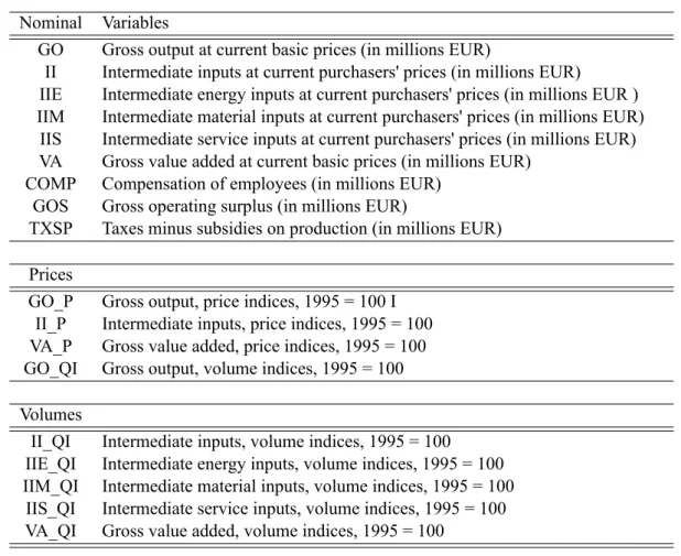
8 Appendix I
Nominal Variables
GO Gross output at current basic prices (in millions EUR)
II Intermediate inputs at current purchasers' prices (in millions EUR)
IIE Intermediate energy inputs at current purchasers' prices (in millions EUR ) IIM Intermediate material inputs at current purchasers' prices (in millions EUR)
IIS Intermediate service inputs at current purchasers' prices (in millions EUR) VA Gross value added at current basic prices (in millions EUR)
COMP Compensation of employees (in millions EUR) GOS Gross operating surplus (in millions EUR)
TXSP Taxes minus subsidies on production (in millions EUR) Prices
GO_P Gross output, price indices, 1995 = 100 I II_P Intermediate inputs, price indices, 1995 = 100 VA_P Gross value added, price indices, 1995 = 100 GO_QI Gross output, volume indices, 1995 = 100 Volumes
II_QI Intermediate inputs, volume indices, 1995 = 100 IIE_QI Intermediate energy inputs, volume indices, 1995 = 100 IIM_QI Intermediate material inputs, volume indices, 1995 = 100
IIS_QI Intermediate service inputs, volume indices, 1995 = 100 VA_QI Gross value added, volume indices, 1995 = 100
Table 1: KLEMS 08I Database
Variables GO K deep L Prod. I.Goods TFP_TOT EFW EF WGI
Production Growth 1.000
Capital Deepening 0.112 1.000
Labor Productivity 0.232 0.044 1.000
Intermediate Goods 0.460 0.062 0.437 1.000
TFP_TOT 0.831 -0.243 -0.149 -0.048 1.000
World Economic Freedom -0.513 0.128 0.178 0.121 -0.670 1.000
Index Economic Freedom -0.209 0.256 0.227 0.041 -0.312 0.723 1.000
Source Indicators Data range Index
Eco-nomic freedom The Index Economic Freedom is composed by ten indicators ag-gregated into four categories. (1) Rule of Law (property rights, freedom from corruption);(2)Limited Government (fiscal free-dom, government spending); (3) Regulatory Efficiency (busi-ness freedom, labor freedom, monetary freedom); and (4) Open Markets (trade freedom, investment freedom, financial freedom). Source: http://www.heritage.org/index/
1995-2012
World Gover-nance Institu-tional Indicators
World Bank Governance Indicators were developed by \citekauf-mann2009 whereas they considered six categories: (1) Voice and Accountability (VA)- accounts for political and civil rights; (2) Political stability and Absence of Violence (PV)- probability of violence or depose a goverment; (3) Control of Corruption (CC)-measures the dimension of public exerpation in prol of private gain; (4) Rule of Law (RL) - considered the enforcement of con-tracts and laws by courts and authorities; (5) Government Ef-fectiveness (GE)- bureacratic measure of the goverments effi-ciency and service quality; (6) Regulatory Quality (RQ)- indi-cators that compreend the effects of market policies. Source: http://info.worldbank.org/governance/wgi/sc_country.asp
1996-2011
Fraser Institute The Frazer Institutes provides the longest institutional Indicators, offering a correction of the older ones using a chain linked in-dex. It scores countries from 1 (very bad) to 10 (excellent) in five categories: 1. Size of Government- extent to which gover-ments reduces the induals economic freedom. (goverment spend-ing, taxes, subsidies, progressivity of taxes etc. ); 2. Legal System and Property Rights- consideres rule of law, property rights and courts; 3. Access to sound money- regards monetary policy and inflationary control thus exchange rate credibility; 4.Freedom to Trade Internationally- open trade is the optimal policy to gain in economic freedom of exchange; 5. Regulation- whether market regulation prejudicial certain markets interfering through subsi-dies or higher taxes by creating a unbalanced market. Source: http://www.freetheworld.com/datasets_efw.html
1970-2010
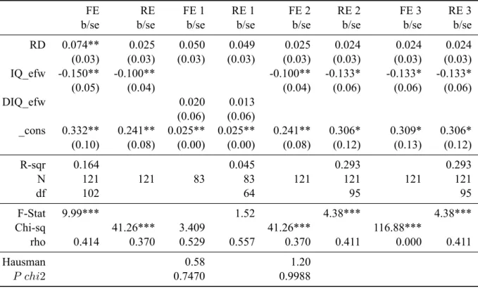
FE RE FE 1 RE 1 FE 2 RE 2 FE 3 RE 3
b/se b/se b/se b/se b/se b/se b/se b/se
RD 0.074** 0.025 0.050 0.049 0.025 0.024 0.024 0.024
(0.03) (0.03) (0.03) (0.03) (0.03) (0.03) (0.03) (0.03)
IQ_efw -0.150** -0.100** -0.100** -0.133* -0.133* -0.133*
(0.05) (0.04) (0.04) (0.06) (0.06) (0.06)
DIQ_efw 0.020 0.013
(0.06) (0.06)
_cons 0.332** 0.241** 0.025** 0.025** 0.241** 0.306* 0.309* 0.306*
(0.10) (0.08) (0.00) (0.00) (0.08) (0.12) (0.13) (0.12)
R-sqr 0.164 0.045 0.293 0.293
N 121 121 83 83 121 121 121 121
df 102 64 95 95
F-Stat 9.99*** 1.52 4.38*** 4.38***
Chi-sq 41.26*** 3.409 41.26*** 116.88***
rho 0.414 0.370 0.529 0.557 0.370 0.411 0.000 0.411
Hausman 0.58 1.20
P chi2 0.7470 0.9988
Output Input Labor Capital TFP Input TFP Labor TFP TFP
GO II HL K GTFP II EMS GTFPII LD GTFP LD GTFP all
Average Growth
1971-1977 18.13% 5.38% 2.09% -1.13% 15.12% . . .
1978-1984 21.74% 2.47% -1.12% 5.78% 19.93% 25.87% 19.94% . .
1985-1991 14.52% 5.08% -1.37% 3.37% 11.54% 37.67% 11.55% . .
1992-1998 7.04% 4.67% -0.59% 6.29% 3.78% 30.20% 3.78% -0.70% 3.70%
1999-2004 4.37% 2.11% 0.85% 6.10% 2.02% 26.93% 2.01% 1.44% 1.56%
Contribution to Gross Output growth
1971 0.078 0.011 0.001 -0.009 0.074
1978 -0.014 0.003 -0.006 0.010 -0.021 0.245 -0.262
1985 0.020 0.003 -0.002 0.003 0.016 0.201 -0.181
1993 -0.002 0.001 -0.009 0.005 0.002 0.192 0.047
1999 0.041 0.007 0.008 0.015 0.011 -0.020 0.038 0.276 -0.256 -0.230
2004 0.023 0.004 0.003 0.006 0.009 -0.083 0.096 0.905 -0.893 -0.806
Contribution to Value Added growth
1971 0.068 0.003 -0.017 0.082
1978 0.052 -0.012 0.019 0.044
1985 0.029 -0.005 0.007 0.027
1992 -0.013 0.211 0.010 -0.018 0.592 -0.593
1999 0.032 0.017 0.032 -0.005 0.404 -0.396
2004 0.017 0.006 0.013 -0.003 1.914 -1.911
Table 5: TFP Growth differences between indicators: Total Industry -- Average growth rate of volumes; Contribution of Input components; and the Total Factor of Productivity calculated using different criteria. Gross Output (GO), Aggregate intermediate input index (II), Hours worked (HL) ICT and ICT -(K), TFP with Capital decomposition (GTFP), Intermediate input decomposed into Energy, Materials and Services (II EMS), TFP with input decomposition (GTFPII), Labor Decomposition (LD), TFP with Labor decompostion (GTFPLD), TFP including all available decomposition -capital, intermediate input and labor (GTFP all). Blank spaces are unavailable data.
GMM1 GMM1_C GMM1_R GMM2 GMM2_C GMM2_R GMM3 GMM3_C GMM3_R
b/se b/se b/se b/se b/se b/se b/se b/se b/se
IQ_efw 0.018** 0.016** 0.041* 0.018** 0.018** 0.041* 0.023** 0.018** 0.041
(0.0) (0.0) (0.02) (0.00) (0.00) (0.02) (0.01) (0.00) (0.03)
RD -0.704 -0.704 -0.573
(0.40) (0.40) (0.78)
F 5995.37*** 685.28*** 21383.3*** 3580.97*** 817.52*** 12496.81*** 8037.36*** 147.1*** 11.72***
Sargan 10.83*** 33.03*** 26.39*** 10.83*** 50.08*** 26.39*** 0.86*** 30.41*** 0.88***
N 1782 1782 1089 1782 1782 1089 1782 1782 1089
AR(2) -0.04*** -0.01*** -1.82*** -0.04*** -0.04*** -1.82*** -0.04*** -0.04*** -1.12***
Inst 19 47 31 19 65 31 19 47 31
Table 6: GMM estimation using Year as a IV: All estimators are clustered sector-wise. GMM1 estimation using only year dummies; GMM1_C is the same model as GMM1 but with collapsed instruments; GMM1_R is the GMM1 controlled by R&D stock. GMM2 estimation using sector and year dummies; GMM2_C is the same model as GMM2 but with collapsed instruments; GMM2_R is the GMM2 controlled by R&D stock. GMM3 controls for both country and year. For all cases the L.TFP has a coefficient of zero and is not significant. Furthermore, we omit the dummy variables. Most had omitted coefficient, but in some rare cases they were significant. legend: * p<0.05; ** p<0.01; *** p<0.001
GMM1 GMM1_C GMM1_R GMM2 GMM2_C GMM2_R GMM3 GMM4
b/se b/se b/se b/se b/se b/se b/se b/se
IQ_efw 0.018** 0.026*** -0.000 0.022** 0.018** 0.018** 0.018*** 0.046*
(0.00) (0.00) (0.00) (0.01) (0.00) (0.00) (0.00) (0.02)
RD 0.559** 0.000 0.000
(0.12) (0.00) (0.00)
F-stat 42389.47*** 3.25e+14*** 6801.19*** 280.33*** 122.91*** 135.89*** 35743.13*** 5685.77***
Sargan 10.83*** 0.00*** 26.39*** 4.62*** 33.00*** 29.99*** 29.99*** 4.62***
Hansen 0.00*** 77.65*** 0.00*** 0.00*** 0.00*** 0.00*** 0.00*** 0.00***
AR(2) -0.04*** -0.58*** -1.57*** -0.03*** -0.19*** -0.94*** -0.94*** -0.03***
N 1782 1782 1089 1782 1782 1089 1089 1782
Instrument 27 21 39 38 66 47 55 46
Table 7: GMM estimation with different combinations of controls and instruments: All estimators are clustered sector-wise. GMM1 TFP is controlled by year and sector, while the IV level is controlled for year and sector effects ; GMM1_C is the same model as GMM1 but with collapsed instruments; GMM1_R is the GMM1 controlled by R&D stock. GMM2: TFP is controlled by year and sector, while the IV level is controlled for year and country effects; GMM2_C is the same model as GMM2 but with collapsed instruments; GMM2_R is the GMM2 controlled by R&D stock. GMM3 and GMM4 controls for country and sector effects, however, IV level is controlled for sector, country and year effects. For all cases the L.TFP has a coefficient of zero and is not significant. Furthermore, we omit the dummy variables. Most had omitted coefficient, but in some rare cases they were significant. legend: * p<0.05; ** p<0.01; *** p<0.001
GMM_efw GMM_efw_R GMM_wgi GMM_wgi_R GMM_ief GMM_ief_R
b/se b/se b/se b/se b/se b/se
L.TFP_sec 0.0 0.0 -24.28 0.0 0.0 0.00
(0.00) (0.00) (40.47) (0.00) (0.00) (0.00)
IQ_efw 0.018** 0.041*
(0.00) (0.02)
IQ_wgi -3.245 -0.117***
(5.21) (0.02)
IQ_ief 0.008** 0.015***
(0.00) (0.00)
RD -0.704 0.325** 0.0
(0.40) (0.07) (0.00)
F-stat 5995.37*** 21383.30*** 37.12*** 37.86*** 5390.95*** 1510.70***
Sargan 10.83*** 26.39*** 10.87*** 13.26*** 18.46*** 15.49***
Hansen 0.00*** 0.00*** 0.00*** 0.00*** 0.00*** 0.00***
AR(2) -0.04*** -1.82*** .*** 0.31*** -2.06*** -2.09***
N 1782 1089 1233 1008 1584 1233
Instru. 19 31 15 15 20 20
GMM IQ IQ_KL IQ_K IQ_R_KL
b/se b/se b/se b/se b/se
IQ_efw 0.018** 0.041* 0.020*** 0.041* 0.046*
(0.00) (0.02) (0.00) (0.01) (0.02)
RD -0.704 -0.704 -0.858
(0.40) (0.38) (0.49)
F-stat 5995.37*** 21383.30*** 1888.72*** 41280.05*** 22142.85***
Sargan 10.83*** 26.39*** 53.66*** 38.24*** 53.81***
Hansen 0.00*** 0.00*** 0.00*** 0.00*** 0.00***
AR(2) -0.04*** -1.82*** -0.04*** -1.87*** -1.99***
N 1782 1089 1782 1089 1089
instru. 19 31 61 46 61
Table 9: The GMM estimation controlling for capital share or/and labor share: Using the System GMM with clustered standard errors by sector, two-step, orthogonal, small sample estimation con-trolling for time effects. We control for either capital share, R&D stock and/or Labor share. In this case, the coefficients of the shares of capital and labor are equal to zero. For all cases the L.TFP has a coefficient of zero and is not significant. Furthermore, we omit the dummy variables. Most had omitted coefficient, but in some rare cases they were significant. legend: * p<0.05; ** p<0.01; *** p<0.001
GMM1 GMM2 GMM3 GMM4 GMM4_R GMM5 GMM6
b b b b b b b
L.TFP_sector 0.00 0.00 0.00 -0.44 0.00 0.00 0.00
RD 0.00 0.00 0.00 0.00
govsize_efw 0.00 0.00
law_efw 0.02* 0.02* 0.00
money_efw 0.02** 0.55* -0.21** 0.01** 0.13**
trade_efw 0.00
creditmkt_efw 0.00
labor_efw 0.65* 0.18* 0.00 0.13*
business_efw 0.00 0.10 0.00 0.00
AR(2) -0.04*** -0.04*** -0.94*** -1.67*** -1.19*** -0.94*** -1.35***
N 1773 1773 1089 1170 999 999 999
Instrument 38 38 47 15 28 44 11