F. C. de Araújo - REPOSITORIO INSTITUCIONAL DA UFOP: New developments on BE/BE multi-zone algorithms based on krylov solvers - applications to 3D frequency-dependent problems.

F. C. de Araújo

Departamento de Eng. Civil/UFOP 35400-000 Ouro Preto, MG. Brazil fcelio@em.ufop.br

W. J. Mansur

C. Dors

and C. J. Martins

Programa de Eng. Civil/COPPE/UFRJ C. P. 68506 21945-970 Rio de Janeiro, RJ. Brazil webe@coc.ufrj.br dors@coc.ufrj.br cj_martins@bol.com.br

New Developments on Be/Be Multi–

Zone Algorithms Based on Krylov

Solvers – Applications to 3D

Frequency–Dependent Problems

In this paper, new developments concerning the use of BE/BE coupling algorithms for solving 3D time–harmonic problems are reported. The algorithms are derived by considering different iterative solvers. Their chief idea is to work with the global sparse matrix of the coupled system, however without considering the many zero blocks associated with the non–coupled nodes of different subregions. The use of iterative solvers makes it possible to store and manipulate only the block matrices with non–zero coefficients. Preconditioned iterative solvers based on the Lanczos, bi-conjugate gradient, and GMRES (generalized minimal residual) methods are used to derive the BE/BE coupling algorithms. A description of the formulation of these solvers, which are completely general and can be applied to any non–singular, non–hermitian systems of equations, is provided. The performance of the algorithms is verified by solving some foundation–soil interaction problems. Important parameters for estimating the efficiency of the algorithms as required CPU times, matrix sparsity, and accuracy of the obtained responses are presented in the results of the paper.

Keywords: Boundary elements–BE, BE/BE coupling algorithms, frequency–dependent analysis, 3D problems, soil–foundations interaction, iterative solvers for complex-valued systems

Introduction

The Boundary Element Method (BEM) is an important numerical tool to perform frequency–domain dynamic analyses of engineering problems, specially those including unbounded domains. Some situations in which frequency–domain or stationary solutions in boundary element applications are necessary are those related to the estimation of resonance frequencies or when time–dependent fundamental solutions are not known, but the corresponding frequency–dependent ones are. For consideration of complex–valued material parameters as e.g. complex stiffness, used for modeling hysteretic damping (Clough and Penzien, 1993), frequency–domain analyses are also suitable. A general review of important papers up to year 1996 on the topic boundary element methods in dynamic analysis, including contributions on frequency– and time–domain analyses, can be found in Beskos (1987, 1997).1

The present paper is concerned with the development of a general and efficient BE/BE coupling algorithm for analyzing time–harmonic problems. Only harmonic loads are considered here. Nevertheless, transient excitations can be also dealt with as a trivial extension of the harmonic case. As a boundary element formulation is involved, the procedure is very suitable for modeling exterior domain problems (infinite domains). On the other hand, the substructuring option (BE/BE coupling) is necessary for taking into account non–homogeneous domains, as e.g. soil layers.

In fact, substructuring strategies extend considerably the range of applications of boundary-integral–based methods. General considerations on subregions techniques can be found in known textbooks on boundary element methods (Banerjee, 1994; Kane, 1994), and in a series of papers published in the last two decades (Crotty, 1982; Kane, Kumar and Saigal, 1990; Rigby and Alliabadi, 1995; Bialecki et al., 1996; Ganguly et al., 1999). These works adopt either non–condensed or condensed strategies and are based on the use of direct solvers.

In previous papers by Araújo and Martins 2000, 2001, and Araújo, Martins and Mansur, 2001, an optimized way for developing generic BE/BE coupling algorithms based on the use of iterative solvers has been reported. In this paper, new advances concerning this BE/BE coupling strategy are presented. The algorithms are derived based on the consideration of different iterative solvers, and their main contribution is that the global matrix of the coupled system is not explicitly assembled; instead, algebraic subsystems corresponding to all its substructures are built and independently manipulated during the solution phase. At the end, the response of the coupled system is assembled. As iterative procedures are used for solving the global system of equations, the coefficients of each subsystem remain unchanged and no additional computer memory, beyond that already allocated for each subsystem, is needed. Non–preconditioned and Jacobi– preconditioned Krylov's solvers, namely the bi-conjugate gradient (Bi–CG), Lanczos, and GMRES (generalized minimal residual) schemes, are applied to derive the generic BE/BE coupling algorithms. A brief description of the formulation of these iterative solvers is provided. In Araújo and Martins (2001), Araújo, Martins and Mansur (2001), and Mansur, Araújo and Malaghini (1992), the complete derivation of the mentioned iterative procedures for real– and complex–valued systems of equations can be found.

The performance of the BE/BE coupling algorithms derived is observed by solving some 3D time–harmonic soil-foundation coupled problems. Important parameters for estimating the efficiency of the computer code, as required CPU times, sparsity of the global matrix, and response accuracy, are presented in the results of the paper.

The Direct Boundary Element Formulation for Frequency-Dependent Problems

The starting expression for frequency–dependent analysis by means of direct boundary element methods is the integral equation

) ( d ) , ( ) , ξ ; ( ) , ξ ( ) ξ

( i ω +

∫

_Γ ik* x ω i xω Γ x

ik U P U

c ) ( d ) , ( ) , ξ ; ( * x x x Γ

=

_∫

_ΓU_ik ω P_i ω +

∫

_ΩUik*(x;ξ,ω)Bi(x,ω)dΩ(x), (1)

where cik is the integral–equation jump term, equal to jump terms for elastostatics, and Uik*(x;ξ,ω) and ( ; , ) * _ξω

x

ik

P are the frequency–

dependent fundamental solutions given by:

(

)

⎩ ⎨ ⎧

−

= _{i k ik}

ik r r

r

U δ

πρ ω

ξ 3, , 4 1 ) , ; ( * _x ⎥ ⎥ ⎥ ⎦ ⎤ ⎢ ⎢ ⎢ ⎣ ⎡ ⎟ ⎟ ⎟ ⎠ ⎞ ⎜ ⎜ ⎜ ⎝ ⎛ − − ⎟ ⎟ ⎟ ⎠ ⎞ ⎜ ⎜ ⎜ ⎝ ⎛ − × 1 1 2 2 1 2 2 2 1 1 1 c r i c r i c r i c r i e c e c r i e e r ω ω ω ω ω ω ⎪ ⎭ ⎪ ⎬ ⎫ ⎟ ⎟ ⎟ ⎠ ⎞ ⎜ ⎜ ⎜ ⎝ ⎛ + ⎟ ⎟ ⎟ ⎠ ⎞ ⎜ ⎜ ⎜ ⎝ ⎛ − + 2 2 2 2 2 2 1 2 1 1 1 1 , , c r i ik c r i c r i k i e c e c e c r r ω ω ω

δ (2)

and

) , ; ( * _xξω ik P ⎥ ⎥ ⎥ ⎦ ⎤ ⎢ ⎢ ⎢ ⎣ ⎡ ⎟ ⎟ ⎟ ⎠ ⎞ ⎜ ⎜ ⎜ ⎝ ⎛ − − ⎟ ⎟ ⎟ ⎠ ⎞ ⎜ ⎜ ⎜ ⎝ ⎛ − × 1 1 2 2 1 2 2 2 1 1 1 c r i c r i c r i c r i e c e c r i e e r ω ω ω ω ω

ω +2

(

6r,ir,kr,m−δikr,m−δkmr,i−δmir,k

)

⎥ ⎥ ⎥ ⎦ ⎤ ⎢ ⎢ ⎢ ⎣ ⎡ ⎟ ⎟ ⎟ ⎠ ⎞ ⎜ ⎜ ⎜ ⎝ ⎛ − − ⎟ ⎟ ⎟ ⎠ ⎞ ⎜ ⎜ ⎜ ⎝ ⎛ − × 1 1 2 2 1 2 2 2 1 1 1 c r i c r i c r i c r i e c e c r i e e r ω ω ω ω ω

ω +2

(

6r,ir,kr,m−δikr,m−δkmr,i−δmir,k

)

⎟ ⎟ ⎟ ⎠ ⎞ ⎜ ⎜ ⎜ ⎝ ⎛ − × 1 2 1 2 2 2 c r i c r i e c c e ω ω m k

ir r

r c i , , , 2 2 ω − ⎟ ⎟ ⎟ ⎠ ⎞ ⎜ ⎜ ⎜ ⎝ ⎛ − 1 3 1 3 2 2 c r i c r i e c c e ω ω 1 1 2 1 2 2 ₁ 2 1 , c r i im k e c r i c c r ω ω δ _⎟⎟ ⎠ ⎞ ⎜⎜ ⎝ ⎛ − ⎟ ⎟ ⎠ ⎞ ⎜ ⎜ ⎝ ⎛ − −

(

)

⎪⎭ ⎪ ⎬ ⎫ ⎟⎟ ⎠ ⎞ ⎜⎜ ⎝ ⎛ − + − 2 2 1 , , c r i km i ik m e c r i r r ω ω δ

δ . (3)

When the known complex boundary conditions

) , ( ) ,

(xω Uxω

U = if x∈Γ₁, (4)

) , ( ) ,

(xω P xω

P = if x∈Γ₂, (5)

are considered, the boundary integral equation (1) gives the solution of the frequency–dependent problem (in terms of its complex amplitudes) at whole boundary.

Adopting usual discretization procedures, the boundary integral equation (1) is converted to the following frequency–dependent system of algebraic equations:

) ( ) ( ) ( )

(ω Uω Gω Pω

H = . (6)

After introducing the boundary conditions shown in equations (4) and (5), equation (6) can be written as

) ( ) ( ) ( )

(ω xω Bω yω

A = , (7)

where the complex vectors x(ω) and y(ω) contain the unknown and known boundary values respectively.

Derivation of Krylov's Solvers for Non-Hermitian Systems

General Aspects

In the computational analysis of engineering systems, continuous models are converted into discrete systems. In this analysis phase, systems of algebraic equations, sometimes sparse, containing a number of equations varying from a few hundreds to a few millions may be originated. Iterative procedures may be very efficient to solve such systems, because, besides preserving the matrix sparsity, they can substantially reduce the CPU time in case of large systems, usual in realistic problems. In Hageman and Young (1981) and Hackbusch (1991), a comprehensive study on general aspects of iterative procedures can be found.

Among the iterative schemes, those classified as Krylov's solvers or polynomial acceleration procedures (Hageman and Young, 1981; Araújo and Martins, 2001) have specially attracted the attention of engineers. The reasons for that is the exceptionally good convergence properties of their preconditioned versions. Important results for non-hermitian BE systems are reported by Araújo and Martins (2001), Mansur, Araújo and Malaghini (1992), Barra et al. (1993), Prasad et al. (1994), and Valente and Pina (2001). In Saad and van der Vorst (2000), a complete review on iterative solvers is provided; more than 200 references are cited.

In this paper, the Lanczos, the biconjugate gradient, and the GMRES algorithms are applied to solve complex–valued, non-hermitian systems of algebraic equations arising in frequency–domain formulations.

The Lancos and Bi-CG Scheme

The starting point for deriving the Lanczos and the bi–conjugate gradient algorithm (Bi–CG) is the Lanczos tridiagonalization algorithm (Araújo, 1989; Wilkinson, 1965). With aid of this algorithm the Lanczos solver is directly derived, and starting from the latter, the Bi–CG scheme can be obtained. Below, a short description of the derivation of their formulation is discussed.

The Lanczos tridiagonalization algorithm can be applied, in the same way as for real matrices, to derive from a matrix A∈CN,N and its transpose, AT, two sequences of complex–valued vectors, {ck+1} and {*ck+1} respectively, given by

1 1

1 + −

+ = − − k k

k k k k

k c Ac α c β c

δ , (8)

1 * * * *

1 * 1

* + −

+ = − − k k

k k k T k

k c A c α c β c

δ , (9)

where c1 and *c1, both in CN, are known initial guess vectors. These sequences of vectors are mutually orthogonal to each other, i.e., ⊥

+1 k

c *c1,*c2, , *ck and *ck+1⊥ c1,c2, ,ck, and thus, linearly independent for k≤N, N being the dimension of the complex space in question. Thus, the following property is verified:

N N

N

C ∈ =

= +

+ _{c 0}

c 1 * 1 . (10)

The property expressed by Eq. (10) is a very important one, since it is concerned with the finite termination of the iterative schemes (Hageman and Young, 1981; Araújo, 1989). Moreover, if an usual inner product is used at the orthogonalization of vectors ck+1 and *ck+1, that is, if for instance a non–hermitian one is considered, expressions for parameters αk, βk and *βk in Eqs. (8) and (9) similar to those for real matrices are obtained. It results (Araújo, 1989; Wilkinson, 1965):

k T k

k T k

k

c c

Ac c

, *

, * =

α , (11)

1 , 1 *

, 1 *

− − − = _kk _TT _kk k

c c

Ac c

β , (12)

1 * , 1

* , 1 *

− − − =

k T k

k T T k

k

c c

c A c

β . (13)

By adopting a three–term iterative formula,

1 1 1

1 1

1 _{(1 )} −

+ +

+ +

+ _{= + + −} n

n n n n n n n

x x

r

x ρ γ ρ ρ , (14)

n denoting the iteration order, and forcing that the associated residual,

1 1 1

1

1 _{( ) (1 )} −

+ +

+

+ _{= − + + −} n

n n

n n n n

r r

Ar

be a Lanczos vector given by Eqs. (8), the Lanczos solver can be derived. Of course, an auxiliary system of equations associated with _AT

must be taken into account; its residual,

1 * 1 * * * 1 * 1 * 1

* _{( ) (1 )} −

+ +

+

+ _{= − + + −} n

n n n T n n n r r r A

r ρ γ ρ , (16)

is forced to be the Lanzos vector given by (9). The parameters in expressions (14)–(16) are then determined by comparing Eqs. (15) and (16) with Eqs. (8) and (9) respectively. It results:

n T n n T n n n Ar r r r , * , * 1 *

1= + =

+ γ

γ , (17)

1 1 , 1 * , * 1 1 * 1 1 1 − − − + + + ⎥ ⎥ ⎦ ⎤ ⎢ ⎢ ⎣ ⎡ ⋅ ⋅ − = = n n T n n T n n n n

n _{γ ρ}

γ ρ ρ r r r r , (18)

with 1ρ₁= and 1 1

r r =* .

By adopting a two–term recursive formula, the Bi–CG scheme is derived. One obtains:

n n n n p x

x +1= +λ , (19)

⎪⎩ ⎪ ⎨ ⎧ ≥ + = = ₋ 1 , 0 , 1 0 n if n if n n n n p r r p

α , (20)

1 1 1 − − − ₋ = n n n n Ap r

r λ , (21)

1 , 1 * 1 , 1 *

1 _{− −}

− −

− = _{n T n}

n T n n Ap p r r

λ , (22)

1 , 1 * , * − − = _nn_TT _nn n

r r

r r

α , (23)

1 * 1 1 * * − − − ₋

= T n

n n n p A r

r λ , (24)

⎪⎩ ⎪ ⎨ ⎧ ≥ + = = = ₋ 1 , 0 , 1 * * 0 0 * * n if n if n n n n p r r r p

α . (25)

The iterative Lanczos and Bi–CG schemes shown above possess the property of being convergent at a maximum of n iterations, where

N

n≤ . Nevertheless, as a consequence of truncating errors introduced during the data processing, convergence may not be achieved for N

n≤ . In order to avoid non–convergence cases and also to accelerate the respective convergence rates, preconditioning strategies have been

taken into account (Araújo, 1989; Mansur, Araújo and Malaghini, 1992; Barra et al., 1993; Prasad et al., 1994). In this work, the only preconditioning matrix Q considered is the Jacobi one, defined by the (real– or complex–valued) diagonal of the respective system matrices.

The GMRES Scheme

Let Kk(r₀,A) be the k–dimensional Krylov's space associated with r0 and A, the complex–valued initial residual vector and the system matrix respectively (Hageman and Young, 1981; Araújo, 1989). By taking an orthonormalized basis v1,v2,…,vk for this subspace, with v₁ given by

0 0 1

r r

v = , (26)

a Krylov's iterative scheme can be generated by imposing the condition:

) , ( 0 1

0 v V y h r A

x

x k k k k

k

i i i

k − =

∑

y = = ∈K

=

with V_k=

[

v₁ v₂ v_k

]

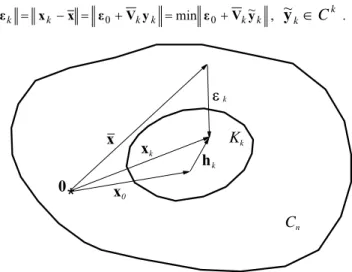
and y_k=(y₁y₂ y_k)T (Hageman and Young, 1981; Araújo, 1989; Araújo and Martins, 2001), where the parameters y₁,y₂, ,y_k are determined according to a certain criterion to be established, and h_k in Eq. (27) is a Krylov's vector (see Fig. 1). Concerning the GMRES solver, y_k is obtained so that x_k be an optimum approximation for x, the exact solution of the algebraic system (see Fig. 1). In other words, the following minimization problem is established: find y_k so that

k k k

k k

k x x ε V y ε V y

ε _min ~

0

0+ = +

= −

= ,

~

y

_k

∈

C

k . (28)

*

x

0

x

x

k

h

k

ε

k

0

K

k

C

n

Figure 1. The k-th iterate x_k and the associated error vector ε_k.

A way to solve this problem is by imposing the condition that ε_k be orthogonal to the Krylov's subspace K_k(v₁,Q−1A), i.e., by considering

0 ) ,

(εk vi = , i=1,2,3, ,k. (29)

By using the Gram-Schmidt orthogonalization procedure to generate the orthonormalized basis V_k, the following solution for the optimization problem above is obtained:

1 0 1

e r H

y_k= _k− , e₁=(1,0, ,0)T, (30)

where H_k is the Hessenberg matrix

⎥ ⎥ ⎥ ⎥ ⎥ ⎥

⎦ ⎤

⎢ ⎢ ⎢ ⎢ ⎢ ⎢

⎣ ⎡

=

kk k k k

k

h h h h

h h

h

3 3

2 22

2

1 12

11

v v

H , (31)

With

) ,

( _{j i}

ij

h = Av v . (32)

GMRES solvers also possess a finite termination property, and the same comments previously done regarding the importance of preconditioning remain valid here. The Jacobi preconditioner is also the only one used in this paper for accelerating the GMRES solver. In order to reduce the number of Krylov's vectors used for expressing the system response, restarting option is considered; namely blocks with a fixed size of N_{30 Krylov's vectors, N being the system order, are adopted.}

Formulation of the Multi–Zone BE Algorithm

[

]

[

]

k k i k b k i k k b k k i k b k i k k b k r p y G B u x H A + ⎪⎭ ⎪ ⎬ ⎫ ⎪⎩ ⎪ ⎨ ⎧ = ⎪⎭ ⎪ ⎬ ⎫ ⎪⎩ ⎪ ⎨ ⎧ ) ( ) ( ) ( , ) ( , ) ( ) ( ) ( , ) (

, , k=1,ns, (33)

where

[

]

⎪⎭ ⎪ ⎬ ⎫ ⎪⎩ ⎪ ⎨ ⎧ = − = ) ( 2 ) ( 1 ) ( ) ( 2 , ) ( 1 , ) ( , , k b k b k b k b k k b k k b k p u x G H

A , (34)

[

]

⎪⎭ ⎪ ⎬ ⎫ ⎪⎩ ⎪ ⎨ ⎧ = − = ) ( 2 ) ( 1 ) ( , ) ( 2 , ) ( 1 , ) ( , , k b k b k b k k b k k b k k b k u p y H G

B , (35)

k

r are the volume forces, and the indexes above are defined as follows: ns is the number of subregions, b₁(k), the outer boundary part of the k-th subregion with unknown displacements, b₂(k), that one with unknown forces, and i(k), its interface (with unknown displacements and forces). Notice that b(k)=b₁(k)∪b₂(k).

As corresponding to the interface nodes of a given subregion k, both displacements and tractions are unknown, an additional number of equations will be necessary for calculating all its unknown boundary values (including, of course, its interface values). In fact the compatibility and equilibrium equations between common subregion interfaces provide the extra equations which permit assembling together the subsystems corresponding to all substructures of the problem. The number of equations and unknowns, after introducing the boundary conditions, become the same and a unique solution to the problem is obtained.

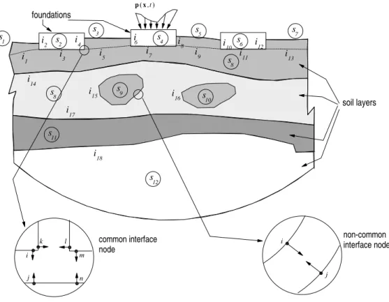
In fact, an interface is defined by a set of coupled nodes, which in turn are defined according to the following criterion: coupled nodes pertain to two different domains, have the same co-ordinates, and the corresponding unit normal outward vectors at them are opposite to each other. For the generic coupled subdomains shown in Fig. 2, the interfaces between the various subdomains are indicated by a global numbering. For instance, interface i₁ is that separating subdomains S₁ and

S

₈, interface i₂, that between subdomains S₁ and S₂, and so on. Explicitly, the global coupled system in its most general form is given by

⎪ ⎪ ⎪ ⎪ ⎪ ⎪ ⎭ ⎪⎪ ⎪ ⎪ ⎪ ⎪ ⎬ ⎫ ⎪ ⎪ ⎪ ⎪ ⎪ ⎪ ⎩ ⎪⎪ ⎪ ⎪ ⎪ ⎪ ⎨ ⎧ ⎥ ⎥ ⎥ ⎥ ⎥ ⎦ ⎤ ⎢ ⎢ ⎢ ⎢ ⎢ ⎣ ⎡ s ns b b b s ns s s ns ns ns b ns b b x x x x x x C C C C C C C C C A 0 0 0 A 0 0 0 A 2 1 ) ( ) 2 ( ) 1 ( , 2 1 2 , 22 12 1 , 21 11 ) ( , ) 2 ( , 2 ) 1 ( , 1 ⎪ ⎪ ⎭ ⎪ ⎪ ⎬ ⎫ ⎪ ⎪ ⎩ ⎪ ⎪ ⎨ ⎧ + ⎪ ⎪ ⎪ ⎭ ⎪⎪ ⎪ ⎬ ⎫ ⎪ ⎪ ⎪ ⎩ ⎪⎪ ⎪ ⎨ ⎧ ⎥ ⎥ ⎥ ⎥ ⎥ ⎥ ⎦ ⎤ ⎢ ⎢ ⎢ ⎢ ⎢ ⎢ ⎣ ⎡ = ns ns b b b ns b ns b b r r r y y y B B B 2 1 ) ( ) 2 ( ) 1 ( ) ( , ) 2 ( , 2 ) 1 ( , 1 , (36)

where s is the total number of existing interfaces, and C_km, the coupling submatrix (containing terms of H_k,i(k) and G_k,i(k)) associated

with the m–th (global) interface. Of course, C_km=0 if the m–th interface does not pertain to the k–th subregion. Regarding the BE model in Fig. 2, C₁₁ and C₁₂ for instance are nonzero, as only the interfaces i₁ and i₂ pertain to subdomain S₁.

) (x,t

p

soil layers foundations

s₁

i

1

s

3

s₄ s₂

s

5

s₆

s

7

s

8

s₉

s₁₀ s₈

s₁₁

s

12

i₂ i

3

i

4

i₅ i

9

i₆ i₇

i

8 i10

i₁₁ i

12

i₁₃

i₁₄

i_{15 i}

16

i₁₇

i

18

i

j n

m l

k common interface node

j

i non-common

interface node

Figure 2. Stratified soil with footings (generic coupled domain).

The continuity and traction conditions mentioned above may be defined as follows: coupling conditions are associated with nodes of the same geometrical position and opposite outward normal vectors; traction continuity conditions, with nodes of same geometrical position and same outward normal vectors. In Fig. 3, these conditions are shown for a generic vector quantity f at nodes i and j. In the computer code, they are automatically introduced into the coupled model.

coupling conditions

i

j

j

i f

f =−

cotinuity conditions

i j

j

i f

f =

s_I

s

II

s_I

s_II

s_III

Figure 3. Coupling and continuity conditions.

First, a coupling examination is carried out so as to identify the coupled nodes and to generate the variables indicating which nodes are coupled with which nodes, and, second, the coupled nodes at which additional traction continuity conditions must be considered are determined and the corresponding variables, generated.

If only non–common interface nodes are present at the model, no traction continuity condition is necessary. Otherwise, that is, in case of common interface nodes, the number of necessary traction continuities is calculated by the formula:

eq var

cont n n

n = − , (37)

Where

= var

n 1 (displacement)+

( )

nnode 2

nsnode

neq= . (39)

In expressions (37)–(39), n_var is the number of variables per common node and n_eq, the corresponding number of equations. nnode and nsnode denote, respectively, the number of nodes and subregions involved at the common interface node. In fact, a common interface node is a nest of coupled multiple nodes. For instance, for the common interface node zoomed in at Figure 2, one obtains: n_var=4 , 3n_eq= , and

1 = cont

n . As from the coupling conditions, pi =−pj , pm=−pn , and pk =−pl , then to calculate ui, pi, pm, and pk, it is necessary to introduce one continuity condition, for example, pi=pm .

Parallel to the ideas above, directly concerned with the description of the coupling process, another strategy is used to completely avoid operating with the many zero blocks, necessarily present at the system (36). In fact, the basic idea to do this is to use iterative solvers, which fundamentally work with no matrix transformation. Thus, the system (36) must not be explicitly assembled. Instead, a loop over the subregions is carried out and the independent contributions of each subregion are taken into account by the operation under consideration (matrix–vector or vector–vector multiplications). At end, the final result of the respective operation is gathered. Notice that no zero block is stored and manipulated during the solution of the system.

In this paper, eight different solvers are actually used in conjunction with the coupling technique; namely, the Lanczos, J–Lanczos, Bi– CG, J–Bi–CG, GMRES, J–GMRES, J–Lanczos(-eq), and J–Bi–CG(-eq). The general description of these methods (Lanczos, Bi–CG, GMRES) is given in the section above on Krylov's solvers for non–hermitian systems. The letter “J” preceding the name of the solvers stands for Jacobi–preconditioning, and the particle “eq”, designates that the real equivalent version of the respective solver is used (Araújo, Martins and Mansur, 2001). If the particle “eq” is omitted, it means that a complex solver is applied.

Applications

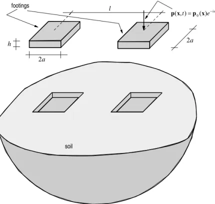
To observe the performance of the coupling algorithms, some problems concerning the dynamic interaction between soil and footings are analyzed (see Fig. 4). As a matter of fact, the following problems are considered: cases of one and two footings, embedded or non– embedded, rigid or flexible, coupled with the soil. In the discretization models adopted, each footing and the soil are considered as one subregion.

footings

a 2

a 2 h

l

soil

t i

e t)= ( ) −ω ,

(x p₀ x

p

Figure 4. Interaction soil–footings under harmonic loading.

Case Study 1: Single Non–Embedded Footing Coupled With the Soil

To validate the computational code developed, a series of analyses in the frequency–domain of a system consisting of a single footing coupled with the soil is carried out. The influence of the footing rigidity on the dynamic response of the system is observed. The relative stiffness of the footing, defined by

3

12 1

⎟ ⎠ ⎞ ⎜ ⎝ ⎛ =

a h E E E

s f

where Ef and

E

s are the elasticity modulus of the footing and of the soil, respectively, and E is used to measure the relative footing stiffness. The dimensionless thickness

a

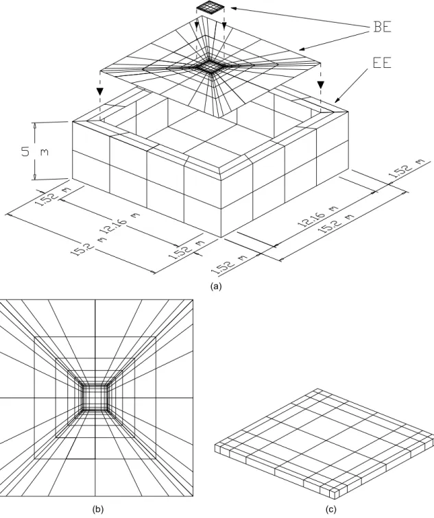
h _{is taken to be 0.10, and the footing is considered to be rigid for E≥1.0. The BE model adopted} to solve this problem is shown in Fig. 5.

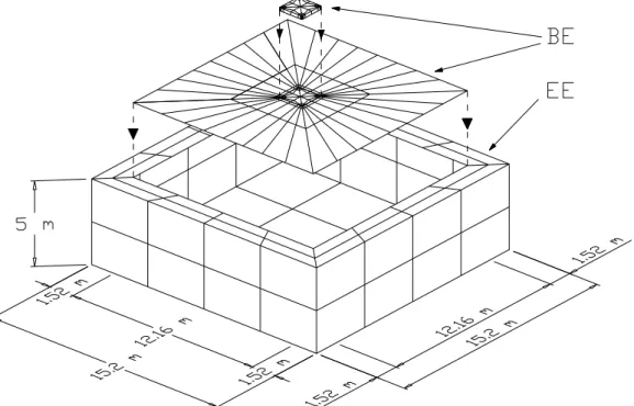
(a)

(b) (c)

Figure 5. Boundary element model:(a) BE and EE meshes; (b) BE mesh for the soil; (c) BE mesh for the footing.

(a) (b)

At the center

0.00 0.05 0.10 0.15 0.20 0.25 0.30 0.35 0.40

0.0 1.0 2.0 3.0 4.0

α0

∆

Prop. method - E=0.016 Prop. method - E=0.240 Prop. method - E≥1.000 Qian et al - E=0.016 Qian et al - E=0.240 Qian et al - E≥1.000 Whittaker et al - E=0.016 Whittaker et al - E=0.240 Whittaker et al - E≥1.000

(c)

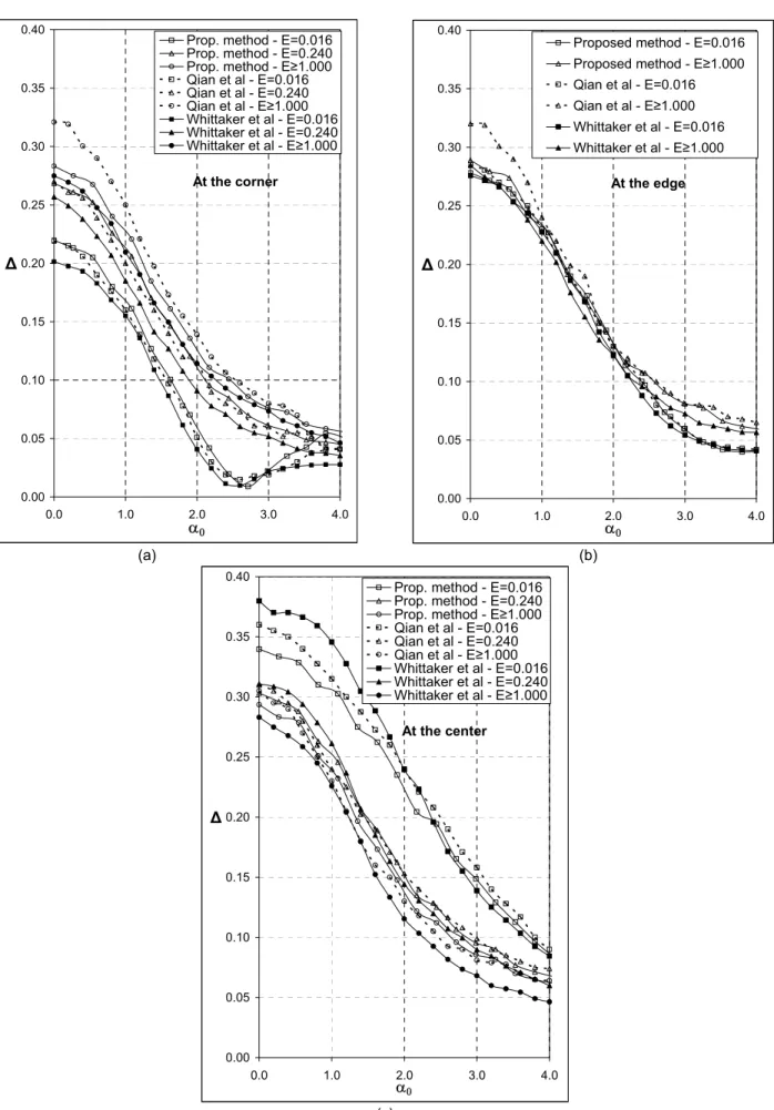
Figure 6. Dimensionless amplitude of the vertical displacement of the footing: (a) at the corner; (b) at the edge middle point; (c) at the center point. At the corner

0.00 0.05 0.10 0.15 0.20 0.25 0.30 0.35 0.40

0.0 1.0 2.0 3.0 4.0

α0

∆

Prop. method - E=0.016 Prop. method - E=0.240 Prop. method - E≥1.000 Qian et al - E=0.016 Qian et al - E=0.240 Qian et al - E≥1.000 Whittaker et al - E=0.016 Whittaker et al - E=0.240 Whittaker et al - E≥1.000

At the edge

0.00 0.05 0.10 0.15 0.20 0.25 0.30 0.35 0.40

0.0 1.0 2.0 3.0 4.0

α0

∆

This problem was also analyzed by Wittaker and Christiano, 1982, and Qian et. al., 1996. Their responses are plotted together with those obtained with the procedure proposed in this paper in the graphics of Fig. 6. In these graphics, the dimensionless vertical displacement amplitude,

∆

, defined through

) 1 ( 4 1

s s

qa w E

ν

+ =

∆ ,

where q is the uniformly distributed load and w the vertical displacement amplitude ∆, is plotted versus the dimensionless frequency,

s c

a

ω α₀= .

with c_s being the shear wave velocity of the soil and a half of the foundation width.

Case Study 2: One Non-Embedded Footing (NEF) Coupled With the Soil

In this case, which aim to show the computational efficiency of the algorithm, a harmonic distributed load of amplitude

2 6 0 4.0 10 Nm

−

× =

p and frequency

ω

=

100

rad

/s, acting in the vertical direction at the top surface of the footing is considered. The physical constants for the footing and the soil are assumed to be:

Soil parameters: E_s= 8 -2

Nm 10 0 .

2 × ,

ν

_s =0.35 and

ρ

s

=

1800

Kgm

−3, cs=202.86m/s

hysteretic damping ζ =0.5% ;

Footing: Ef =Es, Ef =10Es, Ef =50Es, Ef =100Es, Ef =500Es, Ef =1000Es, 35

. 0 =

f

ν and _=1800Kgm−3

f

ρ .

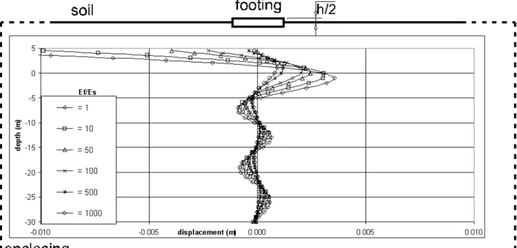
Quadrangular eight–noded boundary elements are used in all problems. The thickness of the footings is h=0.19m and their half side length, a=0.76m, so that α₀ =0.3746.

The model shown in Fig. 7 is considered. The footing (Fig. 9(b)) is discretized with 128 boundary elements (450 nodes), and the soil (Fig. 9(a)), with 144 boundary elements (529 nodes). The enclosing element mesh (EE mesh) contains 48 enclosing elements (161 nodes).

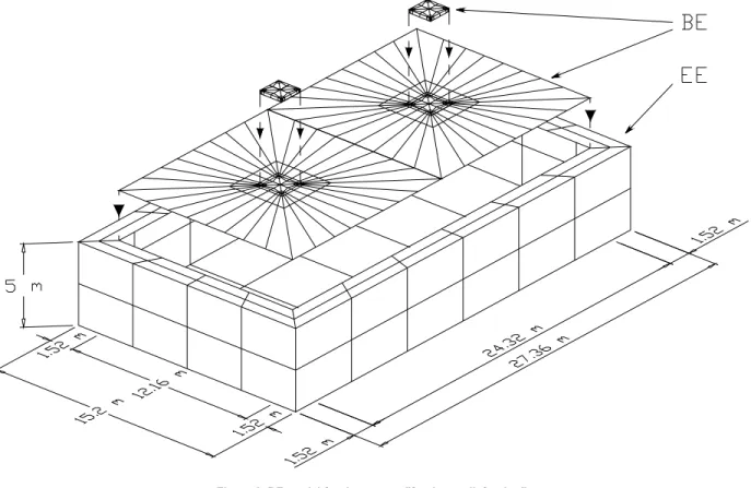
Figure 8. BE model for the system "footing–soil–footing".

(a) (b) (c)

Figure. 9. BE meshes.

Case Study 3: One Embedded Footing (EF) Coupled with the Soil

A BE model similar to that shown in Fig. 7 is adopted. The same loading, geometric and physical characteristics used in case study 2 are also considered here. The BE mesh for the footing contains 160 boundary elements (546 nodes) and for the soil, 176 boundary elements (625 nodes). The EE mesh has 48 enclosing elements and 161 nodes.

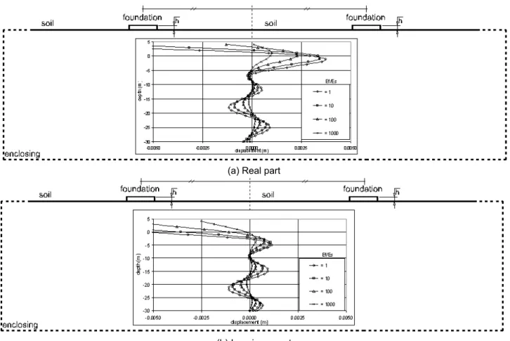
Case Study 4: Two Non-Embedded Footing (2NEF) Coupled with the Soil

The BE model shown in Fig. 8 is used. Again the same characteristics of case study 2 are adopted. Each footing (Fig. 9(b)) is discretized with 128 boundary elements (450 nodes), and the soil (Fig. 9(c)), with 288 boundary elements (1041 nodes). The respective EE mesh has 104 enclosing elements (333 nodes), and the distributed harmonic load acts on both footings.

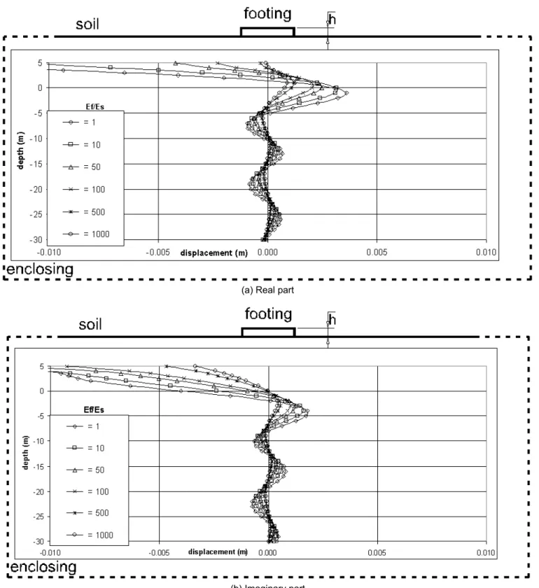
The response of the soil–footing(s) interaction problems for the case studies 2–4 described above is shown by the graphics of Figures 10– 13 in terms of the vertical displacement amplitudes according to the relations E_f/E_s. The sparsity of the coupled systems (defined here as the ratio between the number of zeroes and the total number of coefficients) in the cases 2, 3 and 4 is 31.6%, 26.5%, and 46.5% respectively. The number of iterations (scaled by the system order) and the CPU times (scaled by the corresponding CPU time of the standard Gauss solver with columns and rows pivoting option) attained in the analyses are plotted against the relationship Ef/Es in the graphics 14, 15, 17 and 18.

The iterative scheme was stopped whenever ℜe(rn+1) ≤tol and ℑm(rn+1) ≤tol, with tol=10-5, rn+1 being the residual vector at the current iteration. The computer used for carrying out the analyses had an INTEL processor with 1.0GHz and 768Mbytes random access memory, and the code was developed in a COMPAQ VISUAL FORTRAN environment, version 6.5.0.

(a) Real part

(b) Imaginary part

(a) Real part

(b) Imaginary part

(a) Real part

(b) Imaginary part

Figure 12. Two footings resting on the soil surface – vertical displacement amplitudes below the footings (symmetric).

(a) Real part

(b) Imaginary part

NEF 0 10 20 30 40 50 60 70

0 250 500 750 1000

Ef/Es nu m b er o f i terat io n s sca le d by the s yste m or der (% ) Lanczos J-Lanczos BI-CG J-BI-CG J-GMRES J-Lanczos-eq J-BI-CG-eq EF 0 10 20 30 40 50 60 70

0 250 500 750 1000

Ef/Es

num

ber of i

te rati o ns sc

aled by t

h e sy st em o rde r (% ) Lanczos J-Lanczos BI-CG J-BI-CG J-GMRES J-BI-CG-eq

(a) Non–embedded (b) Embedded

Figure 14. Number of iterations attained by the solvers (values scaled by the system order N).

NEF 0.0 0.1 0.2 0.3 0.4 0.5 0.6

0 250 500 750 1000

Ef/Es it er at ive so lv e r C P U t ime sc al e d b y th e G a u s s one Lanczos J-Lanczos BI-CG J-BI-CG J-GMRES J-Lanc-eq J-BI-CG-eq EF 0.0 0.1 0.2 0.3 0.4 0.5 0.6

0 250 500 750 1000

Ef/Es it e rat iv e solver CPU t ime scaled b y th e Ga us s on e Lanczos J-Lanczos BI-CG J-BI-CG J-GMRES J-BI-CG-eq

(a) Non–embedded (b) Embedded

Figure 15. CPU times measurement of the iterative schemes (values scaled by the Gauss one).

Ef/Es = 1.0

0 100 200 300 400 500 600 700 800 input and domain preparation time coupling searching time continuity searching time matrix assembly time continuity condition time

solver time output time

processing stages (NEF)

CP U ti m e ( sec) Lanczos J-Lanczos BI-CG J-BI-CG J-GMRES J-Lanc-eq J-BI-CG-eq

Ef/Es = 1.0

0 100 200 300 400 500 600 700 800 input and domain preparation time coupling searching time continuity searching time matrix assembly time continuity condition time

solver time output time

processing stages (EF)

CP U ti m e (s ec ) Lanczos J-Lanczos BI-CG J-BI-CG J-GMRES J-BI-CG-eq

(a) Non-embedded

(b) Embedded

NEF

0 5 10 15 20 25

0 250 500 750 1000

Ef/Es

num

ber of

it

erati

ons

scal

ed by t

h

e

syst

em

order (

%

)

J-Lanczos

J-BI-CG

J-GMRES

Figure 17. Number of iterations attained by the solvers: non-embedded footing-soil-footing (values scaled by the system order N).

NEF

0.00 0.03 0.06 0.09 0.12 0.15

0 250 500 750 1000

Ef/Es

it

er

at

ive sol

ver

CPU

ti

me

scal

ed

by t

h

e G

a

uss

one

J-Lanczos

J-BI-CG

J-GMRES

Figure 18. CPU times for the iterative schemes: non–embedded footing-soil-footing (values scaled by the CPU time of the standard Gauss solver).

Ef/Es = 1.0

0 200 400 600 800 1000 1200

input and domain preparation

time

coupling searching

time

continuity searching time

matrix assembly

time

continuity condition time

solver time output time

processing stages (NEF)

CPU t

im

e

(

s

ec)

J-Lanczos

J-BI-CG

J-GMRES

Conclusions

A general procedure is presented to calculate the dynamic response of 3D foundations, rigid or flexible, of any geometrical shape and under any spatial arrangement, coupled with the soil.

The results presented in Figures 10–13 could not be compared with ones furnished by other authors in all cases analyzed, as it was not possible to find all respective results in the technical literature consulted. Nevertheless, the good agreement between the responses obtained with the method proposed here and those furnished by Wittaker and Christiano, 1982, and Qian et. al., 1996 (Fig. 6), ensure the quality of the other responses first published in this paper. This case study was used to validate the procedure implemented.

Concerning the performance of the substructuring algorithm, one sees that convergence was reached at low rates of CPU times, if compared with those attained by using a direct standard Gauss solver (Figs. 15 and 18). Additionally, Figs. 14, 15, 17 and 18 given an interesting insight on how the performance of the solver varies according to the relationship

E

_f

/

E

_s. On the other hand, the coupling procedure proposed is very suitable for developing parallelized BE computer codes. Thus, the procedure might constitute a very promising technique for treating realistic 3D engineering problems via Boundary Element Methods, usually represented by means of algebraic systems of equations with hundreds of thousands of equations. In these cases the factorization or inversion of the resulting system matrix is a very hard computational task, so that the proposed strategy might be very attractive.

Acknowledgements

The first author gratefully acknowledges the financial support from the Brazilian Research Council – CNPq and from the Research Foundation of Minas Gerais– FAPEMIG

References

Araújo, F. C., 1994, “Zeitbereichslösung Linearer Dreidimensionaler Probleme der Elastodynamik mit einer gekoppelten BE/FE-Methode” (in german), Ph.D Thesis, Technische Universität Braunschweig, Germany, 182p.

Araújo, F. C., 1989, “Iterative Techniques for Solving Linear Systems of Equations Originated from the Boundary Element Method” (in Portuguese), M.Sc. Thesis, COPPE – Federal University of Rio de Janeiro, Brazil, 116p.

Araújo, F. C., Martins, C. J. and W. J. Mansur, 2001, “An Efficient BE Iterative-Solver-Based Substructuring Algorithm for 3D Time-Harmonic Problems in Elastodynamics”, Engineering Analysis with Boundary Elements, Vol. 25, pp. 795-803.

Araújo, F. C. and Martins, C. J., 2001, “A Study of Efficiency of Multizone BE/BE Coupling Algorithms Based on Iterative Solvers - Applications to 3D Time–Harmonic Problems”, In M. Denda, M., H. Aliabadi and A. Charafi (eds.), Proc. Joint Meeting of Boundary Element Techniques and International Association for Boundary Elements, New Brunswick–NJ–USA, 16–18 July, Advances in Boundary Element Techniques II, Geneva: Hoggar, Vol.1. pp.21-29.

Araújo, F. C. and Martins, C. J., 2000, “Efficient Generalized Boundary Element Substructure Algorithm for Analysis of 3D Machinery Foundations”, In J. Tassoulas (ed.), Proc. Fourteenth Engineering Mechanics Conference, ASCE, University of Texas at Austin – USA, 21 – 24 May.

Banerjee, P. K., 1994, “The Boundary Element Method in Engineering”, McGraw-Hill Book Company, New York–USA, 512p.

Barra, L. P. S., Coutinho, A. L. G. A., Telles, J. C. F. and Mansur, W. J., 1993, “Multi-Level Hierarchical Preconditioners for Boundary Element Systems”, Engng. Anal. Boundary Elements, Vol. 12, pp. 103–109.

Beskos, D. E., 1987, “Boundary Element Methods in Dynamic Analysis”, Appl. Mechanics Reviews, Vol. 40, pp. 1–23.

Beskos, D. E., 1997, “Boundary Element Methods in Dynamic Analysis: Part II (1986–1996)”, Appl. Mechanics Reviews, Vol. 50, pp. 149–197. Bialecki, R. A., Merkel, M., Mews, H. and Kuhn, G., 1996, “In- and Out-of-Core BEM Equation Solver with Parallel and Non-Linear Options”, Int. J. Num. Methods in Engineering, Vol. 39, 4215–4242.

Clough, R. W. and Penzien J., 1993, “Dynamics of Structures”, McGraw-Hill, Inc., second edition, New York–USA, 739p.

Crotty, J. M., 1982, “A Block Equation Solver for Large Unsymmetric Matrices Arising in the Boundary Element Method”, Int. J. Num. Methods in Engineering, Vol. 18, pp. 997–1017.

Ganguly, S., Layton, J. B., Balakrishna, C. and Kane, J. H., 1999, “A Fully Symmetric Multi–Zone Galerkin Boundary Element Method”, Int. J. Num. Methods in Engineering, Vol. 44, 991–1009.

Hackbusch, W. 1991, “Iterative Lösung Grosser Schwachbesetzter Gleichungssysteme”, B. G. Teubner Stuttgart, Germany, 382p. Hageman, L. A. and Young, D. M., 1981, “Applied Iterative Methods”, Academic Press, Inc., 386pp.

Kane, J. H., Kumar, B. L. and Saigal, S., 1990, “An Arbitrary Condensing, Noncondensing Solution Strategy for Large Scale, Multi-Zone Boundary Element Analysis”, Comput. Meth. Appl. Mech. Engng, Vol. 79, 219–244.

Kane, J. H., 1994, “Boundary Element Analysis in Engineering Continuum Mechanics”, Prentice-Hall, Englewood Cliffs, NJ–USA.

Mansur, W. J., Araújo, F. C. & Malaghini J. E. B., 1992, “Solution of BEM Systems of Equations via Iterative Techniques”, Int. J. Num. Methods in Engineering, Vol. 33, pp. 1823-1841.

Prasad, K. G., Kane, J. H., Keyes, D. E. and Balakrishna, C., 1994, “Preconditioned Krylov Solvers for BEA”, Int. J. Num. Methods in Engineering, Vol. 37, pp. 1651-1672.

Qian, J., Tham, L. G. and Cheung, Y. K., 1996, “Dynamic Cross–Interaction between Flexible Surface Footings by Combined BEM and FEM”, Earthquake Engineering and Structural Dynamics, Vol. 25, pp. 509–526.

Rigby, R. H. and Alliabadi, M. H., 1995, “Out-of-Core Solver for Large, Multi–Zone Boundary Element Matrices”, Int. J. Num. Methods in Engineering, Vol. 38, 1507–1533.

Saad, Y and van der Vorst, H. A., 2000, “Iterative Solution of Linear Systems in the 20th Century”, Journal of Computational and Applied Mathematics, Vol. 123, pp. 1–33.

Valente, F. P. and Pina, H. L., 2001, “Iterative Techniques for 3–D Boundary Element Method Systems of Equations”, Engineering Analysis with Boundary Elements, Vol. 25, pp. 423–429.

Wilkinson, J. H., 1965, “The Algebraic Eigenvalue Problem”, Claredon Press, Oxford.