Bias in Returns to Tenure When Firm Wages and Employment Comove: A Quantitative Assessment and Solution

Bias in Returns to Tenure

When Firm Wages and

Employment Comove: A

Quantitative Assessment

and Solution

Pedro Martins

Andy Snell

Heiko Stueber

Jonathan Thomas

Working Paper

# 601

Bias in Returns to Tenure When Firm Wages and Employment

Comove: A Quantitative Assessment and Solution

Pedro Martins

QMUL, Mile End Road, London and IZA

Andy Snell

University of Edinburgh, 31 Buccleuch Place, EH8 9JT

Heiko Stueber

Friedrich-Alexander Universitat, Erlangen-Nurnburg (FAU) and

the Institute for Employment Research(IAB),

Regensburger Strasse 104, Nuremberg, Germany

Jonathan Thomas

University of Edinburgh, 31 Buccleuch Place, EH8 9JT

March 2016

It is well known that, unless worker-…rm match quality is controlled for, returns to …rm tenure (RTT) estimated directly via reduced form wage (Mincer) equations will be biased. In this paper we show that even if match quality is properly controlled for there is a further pervasive source of bias, namely the co-movement of …rm employment and …rm wages. In a simple mechanical model

where human capital is absent and separation is exogenous we show that positively covarying shocks (either aggregate or …rm level) to …rm’s employment and wages cause downward bias in OLS regression estimates of RTT. We show that the long established procedures for dealing with

"traditional" RTT bias do not circumvent the additional problem we have identi…ed. We argue that if a reduced form estimation of RTT is undertaken, …rm-year …xed e¤ects must be added in order to eliminate this bias. Estimates from two large panel datasets from Portugal and Germany

show that the bias is empirically important. Adding …rm-year …xed e¤ects to the regression increases estimates of RTT in the two respective countries by between 3.5% and 4.5% of wages at

20 years of tenure — over 80% (50%) of the estimated RTT level itself. The results extend to tenure correlates used in macroeconomics such as the minimum unemployment rate since joining

the …rm. Adding …rm-year …xed e¤ects changes estimates of these e¤ects also.

1

Introduction and Overview

A rigorous understanding of returns to …rm tenure - typically regarded as a measure of …rm-speci…c human capital - is important for a host of reasons. In particular it can shed light on the impact of training or on the job learning on labour productivity. Alternatively, it may inform our understanding of the importance of bargaining and rent sharing in …rms. The magnitude of returns to tenure can also determine the importance of the internal labour market compared to its external counterpart. Finally, returns to tenure have important implications in terms of wage inequality, the costs of unemployment and the debate on labour-market segmentation.

Traditionally labour economists use coe¢cient estimates on deterministic tenure in a Mincer equation as a measure of returns to tenure (henceforth RTT). This approach - which we refer to as a reduced form approach - is easy to implement and avoids making structural economic assumptions about worker entry and exit from the …rm. However and as is now well known, the existence of unobservable worker-…rm-match quality means that the OLS regression of wages on tenure gives upward biased estimates of RTT. Several methods — most notably the two step estimator of Topel (1991) and the IV approach of Altonji and Shaktoko (1987) — have been used to circumvent this problem (for a very recent example of an application of both of these methods see Devereux et al., 2013). More recently the emergence of very large panel datasets and advances in computing power have allowed investigators to absorb unobserved worker and match quality by adding …rm-worker match …xed e¤ects (see for example Battisti, 2012).

In this paper we identify a new and potentially pervasive source of bias, namely the existence of a time varying …rm wage component that co-moves with …rm employment. We show that even in a world where match quality is irrelevant, if positive …rm wage/employment co-movements exist, the failure to account for them will bias estimates of returns to tenure downwards. The mechanism generating the bias is the following; …rms that have a relatively high (low) wage at time t (i.e., relative to average wages at that …rm) will have a relatively high (low) employment at t, hence high (low) hiring at t and hence relatively low (high) average …rm tenure at t. Tenure is then spuriously negatively correlated with wages. We show that traditional estimators — ones designed to eliminate the e¤ects of unobservable worker/…rm match quality — are not immune to the bias arising from this e¤ect.

(henceforth FYFE) to wage equations (whilst controlling for worker-…rm match quality) increases estimated tenure e¤ects in the two countries by around 1.5% and 4% of wages, respectively, at 10 years of tenure, and 3.5% and 4.5% of wages at 20 years of tenure. As a proportion of RTT itself these biases exceed 80% for Portugal at ten years of tenure. For Germany the corresponding number is just below 20% rising to 50% at 20 years of tenure. An interesting aspect of our …ndings is that the bias is driven by idiosyncratic …rm level wage/employment co-movement and not aggregate co-movement. An implication of this is that simple …xes such as controlling for the aggregate cycle via the addition of year …xed e¤ects and/or controlling for the level of …rm employment (with a single coe¢cient) will not work. Although investigators may have been aware of some facets of the problem we have highlighted (see for example a discussion in Topel, 1991, on high wage/employment growth …rms or the discussion in Buhai, et al., 2014 on the "size" e¤ect and tenure), to the best of our knowledge we are the …rst to formally analyse it, quantify its importance and propose a simple solution.

A further implication of our results is that using variables that interact macroeconomic variables such as unemployment with deterministic tenure will also result in biased inference. Canonical examples of such variables are Beaudry and DiNardo’s (1991) minimum unem-ployment rate during a worker’s tenure ("minu") and a new hire dummy interacted with unemployment to measure the incremental cyclicality of new hire wages.1 _{In an extension}

to the empirics we quantify these biases as well. The empirical importance of these variates found in the literature adds a further twist because their omission will be yet another source of bias to RTT estimates. We do not model the impact on RTT of omitting these variates theoretically. Instead we quantify the impact in our empirical section.

The key result in this paper – that there is another source of pervasive bias to RTT estimates obtained via reduced form estimation – may lead the investigator to conclude that the safest way to proceed is via a fully speci…ed structural model of worker mobility (see Buchinsky. et al., 2010, for a recent example of such a model). However one key …nding of our work is that it is …rm speci…c (heterogeneous) co-movement that drives the biases we …nd and not macro (aggregate) e¤ects. A structural model with heterogeneous …rm wage/hiring co-movements may be hard to specify and identify empirically. Additionally, estimates obtained from structural models are only as good as the veracity of their underlying assumptions. As far as reduced form modeling goes, our paper has a clear message. To avoid substantial RTT bias one must not only control for worker–…rm match quality (as per tradition) but also for FYFE.

The paper is laid out as follows. Section 2 revisits the traditional econometric model of RTT and the implications for wages. We outline the two canonical estimation methods

1_{Of course if wages are solely determined by a Beaudry Di Nardo style mechanism where an individual}

of Topel (1991) and Altonji and Shakotko (1987) devised to deal with unobserved worker …rm match quality. We then show in section 3 that, in a simple mechanical model with exogenous separation and no human capital (match or …rm speci…c), positive co-movement of …rm wages and employment leads to downwards bias in the RTT estimates whatever method is used. Section 4 contains the empirical results whilst section 5 summarises and concludes.

2

Bias in Estimating Returns to Tenure Arising from

Match Quality

We start with a traditional — and somewhat simpli…ed2 _{— archetypal model of RTT. We}

assume that log wageswijt for worker i in …rmj at timet are given by

wijt = + ijt+ Eit+

0

Xijt+"ijt (Model A)

where "ijt = i+ ij +uijt (Error A)

where ijt is the worker’s tenure, Eit is her lifetime work experience and X is a vector of

other controls. The error consists of a worker …xed e¤ect i, job match quality ij and an

idiosyncratic error uncorrelated with the regressors. Model A makes clear what we mean by RTT. It is the incremental wage received within the …rm by all incumbent workers for each year of completed tenure.3 _{The de…nition may be loosened to allow heterogenous (across}

…rms) tenure related wage growth. In this case the estimates could interpreted as average RTT across …rms with weights given by …rm employment within the sample - analagous to average treatment e¤ects in the experimental literature.

The problem arises when the job match quality ij is correlated with worker i0s tenure.

When the match is good (high ij) the worker’s separation hazard may fall (see in particular

Bowlus, 1995) and expected tenure will rise. This biases upwards the RTT estimate . As noted above one solution to this problem is to explicitly model the entry and exit decisions of workers via a fully speci…ed structural economic model. Following on our previous discussion, here we only consider reduced form estimation. In this context the most popular empirical solutions to the problem of endogenous match quality are the methods of Topel (1991) and Altonji and Shakotko (1987).

Topel’s method …rst di¤erences incumbents’ wages to remove the (presumed constant) match quality and worker …xed e¤ect. Regressing these incumbent wage changes on an

2_{In particular more general speci…cations — as in our empirical section — would include a polynomial in}

tenure whereas for expositional clarity we have a single linear term.

3_{As we have noted already if there are also di¤erential (across tenure) macro e¤ects on wages these must be}

intercept and on Xijt would — in this model at least — produce a consistent estimate of

+ , \+ say. In order to separately identify and , Topel (1991) proposed estimating a second stage regression of wijt \+ ijt on Xijt and the worker’s initial experience on

entry to the …rm. Provided the latter is not correlated with job match quality this produces a consistent estimate of . Subtracting the latter estimate from \+ gives a consistent estimate of the RTT parameter .

Altonji and Shakotko’s (1987) solution to the problem involved using deviations of a worker’s tenure from her ex post time at the …rm as an instrument for tenure itself. Such a variable is by de…nition uncorrelated with both the time invariant job match quality ij and

the worker …xed e¤ect i.4

We now show that the above two methods fail when …rm wages and employment co-move through time. We abstract from complications such as human capital and endogenous worker separation to make clear that the biases we identify exist even in the absence of such e¤ects. The quantitative signi…cance of the bias is an empirical issue which we deal with in a separate section below.

3

Bias Arising from Comovement of Firm Wages and

Employment

We now consider a model that abstracts from the existence of human capital in Model A but that focuses instead on the possible e¤ects of within …rm wage/employment co-movements:

wijt= + ijt+$jt (1)

with i= 1; : : : ; Ljt; j = 1; : : : ; n; t= 1; : : : ; T;

E(Ljt k$jt) = jk; (2)

Ljt =s (Ljt sLjt 1); (3)

Assumption: Ljt >0: (4)

Equation (1) expresses log wage in terms of worker tenure ijt, exogenous survival rate s

(equal to one minus the separation rate) and a …rm speci…c shock$jt. Ljtis …rm employment

at timet.

To …x ideas, and in keeping with much of the relevant data in the area, we considertto be years. The$jt are "equal treatment" components of wages because all workers within …rmj

receive them (see Snell and Thomas, 2010, Hall, 2005, Gertler and Trigari, 2009, Michaillat, 2012 and Gertler, Huckfeldt and Trigari, 2014 for examples of macro theories based on equal treatment and see the latter for empirical evidence in support of it).

4_{In any panel data set the worker …xed e¤ect is subsumed in the job match …xed e¤ect — it is not}

Equation (2) implies that the wage shock $jt may be correlated with current …rm

em-ployment — this is the …rm speci…c wage/emem-ployment co-movement we spoke of above. The equation also allows the wage shock to be correlated with previous employment levels in cases where jk 6= 0. It also allows for the possibility of an aggregate business cycle in wages

and employment. In (3) we specify a constant and exogenous survival (separation) rate s

(1 s), whereLjt is the number of workers at timet with tenure ; and assume in (4) that

separations are never so low or negative employment shocks so large that there is no net new hiring. This (linearity) assumption is made for tractability purposes; if we consider the frequency of observation to be annual then it is not an unreasonable one.5

To simplify we set = 0 (see Model A) so that there is no …rm speci…c human capital embedded in the model and nor is there a return to experience or heterogeneous match quality. This is for clarity; we wish to focus on biases away from zero of the RTT coe¢cient arising because of …rm wage/employment co-movements. We discuss the implications for estimates of returns to experience later. We set = 0 for "new hires" (workers with less than one year of tenure).

The model abstracts from idiosyncratic shocks and …rm speci…c intercepts and common deterministic trends in wages. Adding idiosyncratic (worker speci…c) shocks to wages would not change our results as long as the number of workers in each …rm is large. With regards to common deterministic trends these are typically removed in empirical work via the addition of (common) time trends whilst …rm …xed e¤ects are typically used to extract …rm speci…c intercepts. We would not wish our results to be driven by the existence of these components and so do not model them.

As noted above we assume that the number of workers per …rm per year is large. We need this in order to obtain consistent estimates of …rm speci…c wage components at time t. Given a …xed number of …rms this amounts to assuming N=T is large where N is the total number of panel observations. We wish to derive results in terms of the time series moments of …rm wages and …rm employment. A convenient assumption here would be to assume T itself is large (with T =N _! 0). Although this assumption is counterfactual — panel time spans are typically modest — we do not think it is critical. We could easily drop the largeT assumption and couch our results in terms of sample time series moments rather than theoretical ones. The sign of the bias would then depend on the sign of the sample moments instead of their theoretical counterparts. As it is more common in contexts such as these to derive results based on theoretical moments we prefer to use a large T assumption. Henceforth we take probability limits as N; T _{! 1} and T =N _! 0. We assume we have a panel consisting of all the workers working inn randomly selected …rms during years 1toT.

Casual inspection of the model shows that even in a world free of any kind of human capital, tenure is endogenous; if jk >0 a …rm which has above average wages at timet will

also have above average hiring and below average tenure att.

5_{In the US annual average separation rates are typically in the region of 30%–40% although in Germany}

OLS using demeaned data applied to (1) gives a biased estimate of :6 _{Write the OLS}

estimate as

b_OLS =

T P t=1 n P j=1 Ljt P i=1

( ijt )$jt=N

svar( ijt)

; (5)

whereN =

T P t=1 n P j=1

Ljt is the number of observations, is average tenure in the sample andsvar

denotes sample variance. The denominator in (5) is obviously positive. Denoting average …rm employment per year as Lf =N=nT and recalling that there are L_jt workers of tenure in …rmj at timetwith mbeing the total number of tenure categories7_{, we can rewrite the}

numerator — bN

OLS say — as

bN OLS = 1 Lf T P t=1 n P j=1 m P =0

( )Ljt$jt=nT:

Henceforth we normalise Lf to unity — e¤ectively normalising all of the …rm employment levels. Substituting for Ljt using (3) and simplifying gives

bN OLS = T P t=1 n P j=1 m P =0

( )s _fLjt sLjt 1g$jt=nT

bN OLS = 1 nT T P t=1 n P j=1 m P =1

s _fLjt sLjt 1g$jt

1 nT T P t=1 n P j=1 m P =0

s _fLjt sLjt 1g$jt:

Hence plim_fbN OLSg=

1 n n P j=1 m P =1

s _f j s j 1g

1 n

n

P

j=1

j0:plimf g (6)

where plim_{f g}= s s

m+1

1 s

s

1 s:

Note that the …rst term in (6) does not contain the contemporaneous covariance between …rm wages and …rm employment whilst the second term depends only on this covariance. Note also that the second term (the contemporaneous wage/employment covariance term) is multiplied byplim_f }— typically well in excess of unity — whereas the …rst term’s summed elements are scaled by s — which are strictly less than unity. This gives analytical force to the claims made earlier that contemporaneous wage/employment co-movements are of …rst order importance for the bias and that when these co-movements are positive the bias will be negative.

We examine the bias in yielded by OLS and the two step/IV methods outlined above

for the simple case where non contemporaneous wage/employment covariances are zero, i.e., where jk = 0 for k > 0. This is not to say we believe this assumption to be true. In fact,

adjustment costs and/or other frictions would imply that lagged co-movements would also be correlated with wages. But as (6) shows the …rst order e¤ect on the bias is driven by contemporaneous wage/employment co-movements. We return to the case where wages are correlated with lagged employment in section 4.4 below. There we try and calibrate the bias and for that exercise it will be necessary to additionally control for lagged employment. The analytical results on bias in this section focus only on …rst order e¤ects so that the impact of lagged employment may be ignored.

Our …rst and key result follows directly from (6); if jk = 0 for k >0 (8) implies that

plim_fbOLSg=

0plim_{f g} plim_fsvar_f ijtgg

where 0 =

n

P

j=1

j0

n : (7)

Equation (7) con…rms our intuition that positive co-movement between …rm wages and employment would lead to negative bias in the RTT coe¢cient estimate . However it also shows that the co-movements need not be uniformly positive across …rms for downward bias to exist as long as the average is positive. This is important. It may be that for some …rms, shocks to their labour supply are the dominant in‡uence on their wages rather than from labour demand. This e¤ect might be particularly salient in large …rms that have a degree of monopsony power in their hiring markets.

Now we assess the bias under the Topel (1991) method again taking (RTT) and 0 >0 with k = 0 for k > 0. For the …rst stage we drop new hire (tenure 0) observations and

regress …rst di¤erenced wages on an intercept.8 In this case we show in the annex that

plim_f\+ _g= _f 0

k gs <0 (8)

where k is the proportion of incumbents in the full sample. In the second stage we regress wijt \+ ijt on workeri0s experience on joining the …rm. As \+ is (negatively) biased

the error term becomes$jt+f\+ ) ijt:Under the assumption that a worker’s entry

experience is uncorrelated with his tenure, second stage OLS will give a consistent estimate (of zero) in our setup. The RTT — the di¤erence between …rst and second stage estimates — will be \+ which as (8) shows is negative.

Turning to Altonji and Shakotko’s (1987) IV method we show that ijt ij — where

ij is average tenure for workeri during his time at …rmj — is an invalid instrument under

8_{Usually the RTT are modelled as annth order polynomial function in tenure. In that case we would}

our model. More explicitly we show in the annex that9

plim 1 nT

T

P

t=1

n

P

j=1

m

P

=1

Ljt

P

i=1

( ijt ij)$jt = 0 (s) (9)

where (s) is expected tenure of a new hire — determined by the …xed exogenous survival rates. Not only is the instrument invalid but in this simple single regressor single instrument model — the RTT estimate it produces is downward biased.

3.1

Solution to the Problem: Firm-Year Fixed E¤ects

The source of the bias identi…ed above is the common …rm employment and …rm wage error components.

We propose a general procedure to handle this: estimate Model A but add …rm-year interaction …xed e¤ects. To additionally control for match quality we must also include …rm-worker job match dummies — in e¤ect a two way …xed e¤ects procedure.

However adding match …xed e¤ects in Model A means a loss of identi…cation of the linear experience term . Here we suggest following Topel. Experience should be dropped from the equation and the coe¢cient on the linear tenure term should be used as a consistent estimate of linear experience plus linear tenure, + (^+ say). To separate the linear tenure and experience e¤ects run a second stage regression ofwijt ^+ ijton the worker’s

experience on entry to the …rm. Under the assumption that match e¤ects are uncorrelated with initial experience, this would yield a consistent estimate of . Subtracting the latter from ^+ would give a consistent estimate of — the pure RTT term in Model A. An alternative simpler method — one we pursue below in the empirical section — is to regress the …tted worker-…rm match …xed e¤ects on experience on entry to the …rm. This gives an estimate of the linear experience term which when subtracted o¤ the (linear) tenure term in the two way …xed e¤ects regression gives an estimate of RTT. Additionally this method allows us to test the hypothesis that di¤erent …rms attract workers of di¤erent experience. To do this add …rm …xed e¤ects to the regression of …tted match on experience and see if it signi…cantly changes the estimate of ; if it does not then we would conclude that …rms are homogeneous in terms of the experience of their workers.

3.2

Discussion

First of all we state the obvious. If one is purely interested in e¤ects that vary only with year and tenure then …rm-year e¤ects are uninformative and removing them seems a sensible

9_{We assume for simplicity that there are no partial …rm spells in the data. We could not compute the}

thing to do. Once worker-…rm match quality is controlled for (via match …xed e¤ects) only the cross tenure/year movements in wages are relevant to estimating RTT; components of wages that are common to workers in …rm j in yeart cannot add information.

The second observation is that the use of correlates of tenure in business cycle studies is also subject to the biases we have identi…ed here. Two canonical examples spring to mind. Beaudry and DiNardo (1991) have a contracting model in which the minimum unemployment rate since the worker joined the …rm ("minu") is a su¢cient statistic for wages (modulo human capital). Another example comes from the literature that evaluates a new-hire versus incumbent wage premium; if the new hire wage is (again modulo human capital) found to lie below the incumbent wage in recessions then this has profound implications for models of the labour market because it implies that new hires are able to price themselves into jobs during bad times. New hire/incumbent premia are typically evaluated via the inclusion of a new hire dummy interacted with the unemployment rate (" 0_{u" say) to an otherwise} standard Mincer equation. Both minu and 0_{u are correlates of deterministic tenure and} su¤er from the same problem as the tenure variable itself; coe¢cient estimates will be biased if the workers in a …rm su¤er common wage shocks that covary with …rm employment. It would be particularly interesting if the bias on these terms could be shown to be negative (leading to spurious "right signed" signi…cance) but we cannot show this. In fact, intuitively the opposite may appear true; high …rm wages may be associated contemporaneously with high …rm employment, low (within …rm) average tenure and high (within …rm) averageminu and 0_{u leading to positive bias (bias towards zero). But when one also has to control for} tenure (as surely one must) the sign of the bias cannot be determined.10 _{We leave the sign}

of the bias as an empirical issue — an issue which we ‡esh out in section 4 below.

Thirdly and following on from the previous discussion if variates such as minu and 0_u are important determinants of wages their exclusion will be yet another source of bias to RTT estimates. The omission of relevant regressors that are correlated with included ones will always cause bias so this point is hardly new. Nonetheless for the sake of completeness we assess the quantitative signi…cance of the omission of these two key macro variates on RTT in an extension to the empirics below.

Fourthly our FYFE correction allows for the possibility that …rms may have heteroge-neous wage and employment co-trends. The model in (1) to (4) could easily extend to capture this type of …rm heterogeneity and the end result would be the same — fast (slow) grow-ing and high (low) wage growth …rms would have lower (higher) average tenure and higher (lower) average wages. This type of issue has been discussed before in the RTT literature but as far as we know it has not been analysed.

Finally since the problem is co-movement of wages and employment at the …rm level it would be tempting to simply add …rm employment to the panel regression to purge wages

10_{Simulations of our simple model — available on request — show that when tenure must be additionally}

controlled for negative biases inminuand 0uare possible under plausible …rm wage/comovements. But as

of this variable. It is easy to show that this would only remove the bias if all …rms dis-played the same wage/employment co-movement. Furthermore it may also be the case that wages are correlated with past …rm employment levels as well which would require lagged employment levels to be included. We shall see below in the empirical section that contem-poraneous wage/employment co-movements are in fact very heterogeneous in our German and Portuguese samples.

4

An Empirical Application to German and Portuguese

Panel Data

4.1

Method

In this section we apply our proposed bias correction method — the addition of …rm-year …xed e¤ects — to the RTT estimates from subsamples drawn from two well-used panel data sets; the QP from Portugal and the BeH from Germany. We estimate the following models which allow RTT to be determined as a quartic function of tenure11_:

wijt= ij + 1t+ 2t2+ Age2ijt+

4 P k=1 0 k k

ijt+e0it; (10)

wijt= ij + t+ Age2ijt+

4 P k=1 1 k k

ijt+e1it; (11)

wijt= ij + jt+ Age2ijt+

4 P k=1 1 k k

ijt+e2it: (12)

where ek

it are regression errors

The …rst equation (10) controls for worker-…rm (job match) …xed e¤ects ij and a (quadratic)

time trend (t and t2_{). The second (11) replaces the quadratic trend with more general} year …xed e¤ects t. Speci…cations (10) and (11) are commonly used speci…cations in the

literature. The third speci…cation (12) employs …rm-year …xed e¤ects jt — our proposed

solution to the bias.

The …rm-year …xed e¤ects in (12) will remove i) aggregate (business cycle) time e¤ects in wages ii) …rm and/or sectoral level time e¤ects in wages ii) common trends (stochastic or deterministic) in wages and iv) …rm speci…c wage trends. The square of age (Age2_{) proxies} for the square of experience. Note that the e¤ects of linear experience are absorbed into the linear tenure term 1 but this is not an issue for us: We are interested in the change in the ’s when we add FYFE and if as argued above linear experience is not correlated with

11_{RTT are frequently modelled using a quartic in the literature and we have followed this tradition here.}

either match e¤ects or common wage components then these di¤erences should only re‡ect the bias in the RTT estimate.12

4.2

Data

We draw subsamples from the QP and BeH. For Germany we select all worker spells (see below) in the 100 largest …rms (largest by average employment per year) that existed through-out the entire 1986–2009 time period. For Portugal — where …rms are smaller — we selected all …rms that survived this period and that had a minimum of 100 employees each per year. This gave us 127 …rms. These choices were conditioned by our desire to get a large number of data points each year in each …rm in order to obtain accurate estimates of the …rm year …xed e¤ects. Of course large long-lived …rms may have several RTT characteristics that make them unrepresentative of …rms in the economy as a whole. However we are interested in the di¤erence between RTT estimates from various speci…cations rather than the absolute level. We might also argue that as most workers in the economy work in large …rms results from a sample of large …rms are more "representative" of an economy than would be the results obtained from a random sample of …rms.

We give a brief overview of these two well-used population-based matched employer-employee panel data sets as well as the "cleaning" operations we perform on them.

General features of the data:

The BeH data set is organised by worker spells. A spell is a portion of a year spent at a single …rm. For the BeH if a worker stays with one …rm throughout the year the average daily wage for that "spell" forms a single datapoint. If the worker moves to a second …rm within the year there will be two spells that year; the average wage at each …rm would form a separate datapoint for that year. By contrast the QP is an annual survey that records data on each worker at only one month in the year (March before 1994 but October from 1994 onwards). For QP then there is only one worker "spell" per year.

The BeH draws data from the total gainfully employed members of the German popu-lation who are covered by the social security system. Not covered are self-employed, family workers assisting in the operation of a family business, civil servants (Beamte) and regular students. We focus solely on workers employed in states of the former West Germany. The BeH covers roughly 80% of the German workforce. Plausibility checks performed by the social security institutions and the existence of legal sanctions for misreporting guarantee that the earnings data are very reliable — in contrast with interview based wage data such

12_{Buhai et al. (2014) argue that the (log of the) normalised worker tenure rank is an important}

determi-nant of wages when added to traditional tenure speci…cations. Although signi…cant, the e¤ect they …nd is quantitatively small (moving from being the "newest" to the "oldest" worker adds about 2% to the wage). Adding this term would likely decrease our estimates of the level of RTT. However because such a vari-ate is orthogonal to $jjt (the common …rm wage component), the bias in RTT- which is the focus of our

as that in, say, the PSID (for the US) or the SOEP (for Germany).

Unfortunately the BeH only documents total spell earnings and not hours worked in that spell. We therefore only consider full time workers. Nearly all full time workers in Germany work a standard number of hours per week so the average daily wage should be very closely related to the hourly wage. To calculate the daily real wage (in 2005 prices) we use the Consumer Price Index (CPI). Unfortunately wages are censored at a maximum level equal to the contribution assessment ceiling of the compulsory pension insurance scheme. Earnings spells with wages above or close to (within 1% of) the truncation point are dropped. We drop all spells that have missing tenure. Unfortunately this means a worker only enters the data when he joins a …rm after Jan. 1, 1975.13 _{For this reason we drop the …rst 12 years}

and use worker spells dated at 1986 and beyond.

The QP covers all workers except the self-employed and those employed in the public sector; of course, the unemployed and the inactive are also not included. There are several wage variables, all of them expressed in monthly values (the most common type of pay in Portugal), including base wages, tenure-related payments, overtime pay, subsidies and ‘other payments’ (this latter category includes bonuses and pro…t- or performance-related pay). All QP wages have been de‡ated using Portugal’s CPI and are expressed in 2005 euros. There is also information about normal hours and overtime hours per month. The benchmark measure of pay adopted in this study is based on the sum of all …ve types of pay divided by the sum of the two types of hours worked, resulting in a measure of total hourly pay. Tenure is measured (in rounded years) as the current year minus the reported start year.

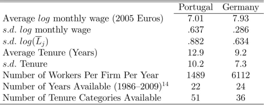
The Table below gives a brief summary of the datasets’ main features. Averages and standard deviations are taken over job spells.

Table 1: Data Summary Statistics

Portugal Germany Average log monthly wage (2005 Euros) 7:01 7:93

s:d: log monthly wage :637 :286

s:d: log(Lj) :882 :634

Average Tenure (Years) 12:9 9:2

s:d: Tenure 10:2 7:3

Number of Workers Per Firm Per Year 1489 6112

Number of Years Available (1986–2009)14 _{22 24}

Number of Tenure Categories Available 51 36

Note: Lj is average annual employment of …rm j.

13_{For the analysis we only use the years 1986–2009, but for the identi…cation of …rm entrants and the}

Table 1 shows some stark di¤erences in the two labour markets. Aside from average wages being very much lower in Portugal (as we would expect) wages are over twice as volatile there. Average tenure however is very high in both countries. Separation rates are around 10%; much lower than the 30% level in the US (see for example Hobijn and Sahin, 2007). Firms are not only very much smaller in Portugal but also vary in size more than they do in Germany. We will return to some of these di¤erential features below.

4.3

Estimates

In this section we estimate a variety of wage on tenure speci…cations and extract …tted values of the (quartic in) tenure component. As noted already these …tted values incorporate the e¤ects of linear experience. For clarity and correctness we refer to these …tted values as "RTTE" — "returns to tenure plus linear experience".

The number of yearly tenure categories available from BeH and QP were 51 and 36 respectively. We start by estimating the "Base" speci…cation (10) and comparing with the speci…cation where we add …rm year …xed e¤ects (henceforth the FYFE speci…cation) equation (12) above. Table 2 below displays the results for the four tenure terms

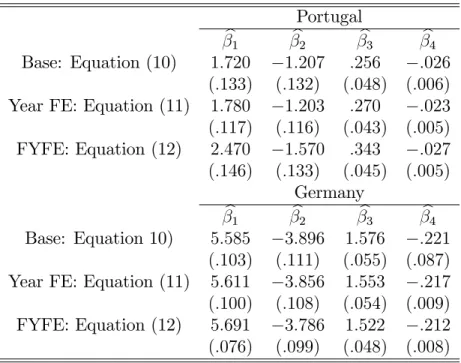
Table 2: Estimates of Tenure E¤ects for Germany and Portugal

Portugal

b₁ b₂ b₃ b₄

Base: Equation (10) 1:720 1:207 :256 :026

(:133) (:132) (:048) (:006)

Year FE: Equation (11) 1:780 1:203 :270 :023

(:117) (:116) (:043) (:005)

FYFE: Equation (12) 2:470 1:570 :343 :027

(:146) (:133) (:045) (:005)

Germany

b1 b2 b3 b4

Base: Equation 10) 5:585 3:896 1:576 :221

(:103) (:111) (:055) (:087)

Year FE: Equation (11) 5:611 3:856 1:553 :217

(:100) (:108) (:054) (:009)

FYFE: Equation (12) 5:691 3:786 1:522 :212

(:076) (:099) (:048) (:008)

Note: Standard errors, clustered by tenure, are in parentheses. bk and standard errors are

scaled by 10k+1_.

con-trast adding FYFE to Base causes quantitatively important changes in many of the tenure estimates. This is particularly true for Portugal; here the …rst three tenure terms are about 25% higher in absolute value in the FYFE compared with Base and the 95% con…dence intervals for the FYFE linear and quadratic terms do not include their Base counterparts. The German estimates change far less and the Base and FYFE con…dence intervals for each parameter overlap.

However, changes in the individual parameter estimates per se tell us little directly about changes in the RTTE. To get a better handle on the impact of adding FYFE to overall RTTE estimates we plot the implied di¤erence in RTTE estimates (FYFE minus Base) against tenure (in years). Henceforth we refer to these di¤erences as the "bias" (although this is somewhat erroneous as it is in fact the negative of the bias15_).

We do not have exact standard errors for the bias but we can obtain an upper bound for them as follows. We show in the annex that under the null hypothesis of no bias the covariance matrix of the Base RTTE estimates exceeds that of the bias by a positive de…nite matrix. The variance of the bias will in this case have an upper bound equal to the variance of Base RTTE estimates. Given that the RTT estimates at each tenure level are merely linear combinations of the tenure parameters we can use the Base covariance matrix to construct 90% and 95% upper bound con…dence intervals around the bias. Figures 1 and 2 display the di¤erences in RTTE estimates (FYFE minus Base) together with their 90% and 95% upper bound con…dence intervals for Portugal and Germany respectively. Figures 3 and 4 plot graphs for FYFE minus Year FE again with upper bounds 90% and 95% con…dence intervals16_.

The bias is positive and rises with tenure in both countries. At a tenure of 10 years the bias rises to about 4.0% of wages in Portugal and 1.7% in Germany. At 2017 _{years of}

tenure the German bias rises to above 3.5% In terms of statistical importance, the bias is highly signi…cant at the 95% level for Portugal but has borderline signi…cance for Germany. However the German biasis signi…cant at the 90% level. Given that the con…dence intervals are upper bounds and that our prior view was that Base RTTE estimates would be downward biased (motivating a one tailed test and use of the 90% level) we could justi…ably argue that the bias is signi…cant for both countries.

Recall that our linear tenure terms also included the e¤ects of linear experience. To get estimates of the level of RTT itself, "pure" RTT, we …rst of all need to get an estimate of the e¤ect of linear experience. To do this we follow the second suggestion advanced in section 3.1: Regress …tted match e¤ects on experience at the time of entry to the …rm. Doing so gives linear experience estimates of just above0:7%per year in Portugal and2:2%per year in

15_{It is also erroneous in that it implies that there are no other sources of bias. Our claim here is to have}

identi…ed a major and pervasive source of bias to RTT rather than an exclusive source.

16_{The variance result we derive in the annex for the FYFE minus Base case is easily adapted to the FYFE}

minus Year FE case. We do not o¤er a proof but one is available on request.

17_{We do not analyse results beyond 20 years of tenure. The numbers of workers in tenure categories above}

Germany. Subtracting these experience estimates from the tenure estimates obtained from (12) gives us our "pure" RTT estimate. For workers of ten years tenure the pure RTT is just over 5% for Portugal and about 9% for Germany. These estimates show how quantitatively important the biases are; for Portugal (and again for workers of ten years of tenure) the bias is over 80% of its pure RTT counterpart whilst for Germany it is about 20% rising to 50% at very long (20 years) tenure.

Finally and as an aside we note a feature of the estimation of the linear experience term. We found that adding …rm …xed e¤ects to the regression of …tted match values on experi-ence at entry to the …rm made little di¤erexperi-ence to the experiexperi-ence coe¢cient. This suggests there is no heterogeneity amongst …rms in terms of their tendency to hire experienced or inexperienced workers.

4.4

Exploring the Source of the Bias: The Role of Firm

Employ-ment

The analytical arguments above pointed to co-movements in …rm wages and employment as the source of the problem. In this section we see the extent to which current and lagged …rm employment can account for the bias. We do this in two ways. First we control for current and once-lagged …rm employment levels in the Base speci…cation and see what e¤ect it has in terms of reducing the bias. Secondly we calibrate the bias by plugging estimates from this augmented Base speci…cation (together with other data moments from the panel) into our simple analytical model above.

A …rst pass at removing the bias might be to purge …rm wages of the e¤ects of …rm employment by adding the latter as a regressor to the Base speci…cation18_{. Adding a single}

term in (log of)19 _{…rm employment to Base alters the RTTE estimates little;}20 _{the bias is}

reduced by no more than 10% in either country at any tenure up to 20 years. Adding lagged …rm employment is equally impotent in this respect. This suggests that if wage/employment co-movements are the source of bias then such co-movements must be heterogeneous across …rms. We now explore this issue further.

We estimate a model that allows for heterogeneous and dynamic …rm wage/employment

18_{For example, in their analysis of seniority and using the QP, Buhai et al. (2014) add a single term in}

…rm employment to control for what they call the …rm size e¤ect on wages.

19_{The theoretical analysis is in terms of employment levels normalised by average …rm employment, L}f_.

Using logs (and hence estimating elasticities) is an approximation therefore.

co-movements. Explicitly we estimate

wijt= ij + Age2ijt+

4 P k=1 0 k k ijt+ n P j=1 0

jdjtljt+

n

P

j=1 1

jdjtljt 1+ 1t+ 2t2+e0it; (13)

where djt is a dummy equal to 1 when the wage is drawn from …rm j and zero otherwise

and where ljt is log of …rm j’s employment at t: We call this regression the "Employment"

speci…cation. Estimating (13) has a treble purpose. First we wish to see the extent to which absorbing wage/employment co-movements reduces bias. Second we wish to establish the ex-tent of heterogeneity of wage/employment co-movements. Thirdly we wish to obtain "good" estimates of wage/employment elasticities for a calibration exercise. The key parameters for the calibration are the ₀j terms. In order to obtain consistent estimates of these we need to nest as much of the employment/wage co-movements as possible in (13). Limiting the lag length in (13) to one is driven in part by prior theoretical reasoning and in part by degrees of freedom constraints. We e¤ectively have only 22 (24) time series observations with which to estimate each …rm’s ’s so two ’s per …rm would seem a reasonable choice on degrees of freedom grounds. With regards to prior reasoning, hiring costs and or labour adjustment costs would suggest that current and lagged employment are the prime correlates of current wages.

We estimated (13) and recomputed the bias (Employment RTTE minus Base RTTE). The results are in Figures 5 and 6. We add the "FYFE minus Base" line to Figures 5 and 6 for comparison. Looking at the Figures we see that adding the employment terms produces RTTE estimates very close to those obtained in the FYFE speci…cation for Germany — e¤ectively removing the bias. For Portugal the results are less de…nitive but even so the extra terms reduce the bias by over 70% at 20 years of tenures.

Turning to heterogeneity, Figures 7 to 10 show the distribution across …rms of the es-timated employment elasticities 0

j and j1 for each country. We see from the Figures that

there is indeed a diverse pattern of wage/employment co-movements across …rms.21

Inter-estingly the average contemporaneous elasticity — an estimate of 0 — is positive in both countries (:073 for Portugal and :011 for Germany). This is consistent with downward bias in estimates of RTTE.

At the risk of taking our simple model too seriously we calibrate the bias using estimates from (13) and sample moments to see if we can match the bias we saw in the Base speci…ca-tion. The general form for the bias is given in equation (6). Adapting it to the case where

21_{Standard errors of the elasticities (the ’s) in both the Employment speci…cation (and}

j0 and j1 are the only nonzero employment/wage covariances gives

plim_fbOLSg=

1 n

n

P

j=1 s j1

1 n

n

P

j=1

j0plimf g

!

=plim_fsvar( ijt)g

= (s 1 0plimf g)=plimfsvar( ijt)g: (14)

We plug estimates from (13) into equation (14) together with data sample moments to

calibrate the bias. Explicitly we estimate 0 with

n

P

j=1b 0

j=n and 1 with

n

P

j=1b 1

j=n, whereb

denote an OLS estimate from (13). We use Hobijn and Sahin’s (2007) estimates of annual separation rates for Portugal and Germany of:11 and :12respectively giving survival rates,

s; of :89 and :88. Finally we estimate plim_fsvar( ijt)g with its sample counterpart from

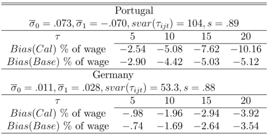
Table 3: Calibrating The Bias

Portugal

0 =:073; 1 = :070; svar( ijt) = 104; s=:89

5 10 15 20

Bias(Cal) % of wage 2:54 5:08 7:62 10:16 Bias(Base) % of wage 2:90 4:42 5:03 5:12

Germany

0 =:011; 1 =:028; svar( ijt) = 53:3; s=:88

5 10 15 20

Bias(Cal) % of wage :98 1:96 2:94 3:92 Bias(Base) % of wage :74 1:69 2:64 3:54

Table 3 shows that for Germany the calibrated bias …ts its empirically estimated coun-terpart extremely well over all tenures. For Portugal the …t is reasonably good up to 10 years of tenure but above that is poor. There are two features of the simple model that may be behind this last result. Firstly — despite its quadratic form — the estimated RTTE for Germany is close to being linear for tenures up to 20 years whilst that for Portugal is dis-tinctly nonlinear. Our analytical model has of course only one (linear) tenure term. Second the simple model assumes equal size …rms (on average) but Table 3 shows that the standard deviation of thelog of average …rm employment is 25% higher in Portugal than in Germany. One …nal problem could be that higher order lags are missing for Portugal’s Employment speci…cation leading to a poor estimate of the crucial 0

j parameters. This last fact may also

be the reason only 70% of the bias is removed by the Employment speci…cation.

Despite the over prediction of the bias at long tenures for Portugal the simple analytical model appears to have had some traction in explaining the origin, sign and magnitude of the empirical bias we have discovered in RTTE estimates.

4.5

Tenure Correlates:

minu

and

u

We argued above in section 3.2 that estimates of macro tenure correlates such as minu and 0_{uwill be subject to similar biases as tenure itself.}

To illustrate biases that may arise we once again use our simple model in (1) to (4) as the data generating process and estimate by pooled OLS:

wijt = + ijt+ kukijt+$jt (15)

where k =minu; 0

u and where uminuijt (u 0

u

ijt) is the value of worker i’s minu ( 0u) at time t

We can show using textbook formulae that the bias in k _{can be written as}

(bk

OLS k)/ wuk _{w u}k

where _/ means "positively proportional to" and xy is the correlation coe¢cient between

x and y. We can view these correlation coe¢cients through the lens of our simple model. If we assume once more that 0

j > 0 but kj = 0, k > 0; then removing the e¤ects of

aggregate shocks by adding Year FE reduces the bias in absolute value.22 _{However the}

sign of the e¤ect of moving to a speci…cation with FYFE (i.e. controlling for idiosyncratic …rm wage/employment co-movements) is indeterminate: The terms w and uk are both

negative (the former we have demonstrated already and the latter derives from the fact that uk _{is weakly decreasing with tenure) whilst}

wuk is positive which implies we cannot

determine the sign of the impact of idiosyncratic co-movements on the bias. We repeat our earlier contention that in the context of estimating the e¤ects of variates that move only over time and tenure, common wage components are at best noise and at worse bias-causing. These wage components should be removed whatever the sign of the bias. We now assess the impact on of doing so.

In macroeconomic applications involving minu and 0_{u it is important to additionally} control for the aggregate business cycle. We do this by adding Year FE to our new Base speci…cation. Explicitly we addminuand 0_{uto (11) and (12). Table 4 displays the results.}

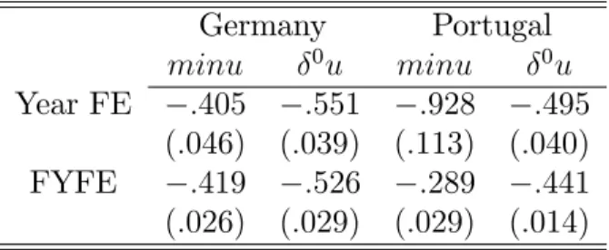
Table 4: Bias in minu and 0_u

Germany Portugal

minu 0_{u minu} 0_u

Year FE :405 :551 :928 :495

(:046) (:039) (:113) (:040)

FYFE :419 :526 :289 :441

(:026) (:029) (:029) (:014)

All estimates are highly signi…cant although quantitatively small. For Germany, adding FYFE changes little in either estimate but in Portugal and forminuthings are di¤erent; the FYFE estimate is less (in absolute value) than one-third of its Year FE value. Portugal’s

0_{uvalue also moves towards zero but far less — by only 10% or so of its original value.}

We close by returning to a point made in the initial discussion of macro variates above. We argued that omission of relevant tenure correlated variates such as these will cause further bias to RTT. Controlling for tenure related macro e¤ects is a two way street: failing to control for FYFE may bias their estimates whilst omitting these variates may bias estimates of RTT. Figures 11 and 12 display the di¤erences in RTTE estimates we get when we add each respective macro variate to the FYFE speci…cation in (12). Adding 0_{u clearly reduces}

RTT by a non negligible amount — up to 3% (1.5%) of wages for Germany (Portugal). Adding minu has far less impact — less than a 1% reduction in both countries. Clearly it is important to control for tenure related macro variates if one wishes to obtain good RTT estimates.

Finally we should check that adding FYFE to the Year FE speci…cation continues to make a di¤erence even in the speci…cations containing minu and 0_{u. Figures 13 and 14} show the di¤erence in RTTE we get when we add FYFE to the Year FE speci…cation in the minu= 0_{u speci…cations (marked as "Minu"/"Deltau" on the graph). For comparison} we add the line showing the impact of adding FYFE (moving from (11) to (12)) when the macro terms are absent (marked as "No Macro" on the graph). The Figures con…rm emphatically that addition of FYFE remains important despite the addition ofminuand 0_u to the speci…cations. In fact the impacts are practically the same as those found originally in section 4 except for the case of minu in Portugal. Here adding FYFE to the Year FE increases RTTE by over 6% at long tenures compared with an original impact (absent macro variates) of just over 4%.23

We summarise by saying that adding tenure related macro e¤ects is important in order to get good estimates of RTT. Likewise adding FYFE is essential to get good estimates of both RTT and tenure related macro e¤ects.

5

Summary and Closing Comments

We have shown that failing to control for co-movement of wages and employment at …rm level leads to downward bias in RTT estimates obtained from reduced form wage equations. We also argued the same mechanism could also bias the coe¢cients on correlates of deterministic tenure such as minu and 0_{u. Our estimates from all the wrokers in 100 or so large long} lived Portuguese and German …rms imply that these biases are quantitatively important. In other words, our …ndings indicate that the importance of tenure in terms of wages has been substantially underestimated in the existing literature. Given that this literature informs issues involving internal labour markets, rent sharing, training and institutional dimensions in labour market outcomes then obtaining more rigorous measurement of the e¤ects of tenure using the methods we propose here would seem to be important.

We conclude on a warning. In another exercise we drew a set of small random worker-based random subsamples from our main dataset and re-estimated equation (12) - i.e. con-trolling for FYFE - each time. The variation in RTT estimates was very high. There seems to be an incidental parameter problem here. Small worker-based random samples o¤er few observations per …rm per year. As a result the FYFE will be poorly estimated. This suggests that when obtaining reduced form estimates of RTT a (large) …rm based samples rather than

23_{This is of course a mirror image of the large impact that adding FYFE has to theminuestimate in the}

Appendix

Bias using Topel’s Method

plim_f\+ _g= 1 kplim T P t=1 n P j=1 m P =1

Ljt $jt=nT

= 1 kplim 1 T T P t=1 n P j=1 m P =1

s (Ljt sLjt 1) $jt=n

= _f 0

k gs <0:

Bias using Altonji and Shakotko’s method

Note that workers joining …rm j att all have the same expected tenure. The average of …rm tenure for workers joining attwill therefore be a constant t plus ano(1)term. We use

this fact below:

A= 1

(PLt)=nT

1 nT T P t=1 n P j=1 m P =1 Ljt P i=1

( ijt ij)$jt

= 1 nTf T P t=1 n P j=1 m P =1 Ljt P i=1

ijt$jt T P t=1 n P j=1 m P =1 Ljt P i=1

ijt$jtg

using plim ijt = (s)

plimA= 1

nT:0 (s)plim 1 nT T P t=1 n P j=1 m P =1 Ljt$jt

!

= (s)plim 1

nT T P t=1 n P j=1 m P =0

$jt(Ljt sLjt 1)

!

= 0 (s)<0:

Proof that the variances of FYFE minus Base tenure estimates are less than those of Base

We start with model (10). We expand the error terme0

it into two components ijt and!jt

— an idiosyncratic worker shock and a …rm-year "shock". Under the null these shocks are mutually uncorrelated and uncorrelated with the regressors (we consider the match e¤ects to be regression dummies):

wijt= ij + Age2ijt+

4 P k=1 0 k k

If we put the four tenure terms, the square of age and the worker …rm match dummies into a single regressor matrix X say with the …rst four columns being the occupied by the (quartic) tenure terms, we can write the Base regression model in the familiar textbook form:

y=X +u=X + +!;

using obvious notation.

Now pN(bOLS )has the standard form:

p

N(bOLS ) =

X0_X

N 1

X0_{( +!)}

p

N :

Writing ! = Z where Z is a regressor matrix containing …rm-year dummies24 _with

coe¢-cient vector we get the augmented regression model

y=X +Z + :

Denote the estimate for from this new regression as . We can obtain the OLS estimate of in a roundabout (two-step) way. First regressyonX andZ. Then compute the …tted values! =Z . Run a second regression

y=X +! + :

The estimate of will be unity whilst the estimate of will be numerically identical to and will obviously have the same distribution. The next thing to note is that under the null plim_fX0!

N g= 0. So we have

plim_fX

0

!

N g= 0:

In short the textbook X prime X matrix is asymptotically block diagonal. We can therefore

write pT( ) as

p

N( ) = X0X

N 1

X0

p

N +o(1):

Using the fact that under the null both bOLS and are consistent we can write the di¤erence

between the two estimates as bOLS = ( ) (bOLS ) so that

p

N bOLS =

p

N ( ) (bOLS )

= X

0_X

N 1

X0_!

p

N +o(1):

24_{We must drop two FYFE dummies becauseX includestandt}2

Recall from above thatpN bOLS = X

0_X

N

1 _X0_{(!+ )}

p

N . But under the null! and are

mutually uncorrelated. This means that

vcovpN bOLS vcov

p

N bOLS =A+o(1);

where A is a positive de…nite matrix. Finally note that the RTT estimate at tenure evaluated at some estimated coe¢cient vector is just

RT T( ; ) = ( ; 2; 3; 4;0;0; : : : ;0) :

It follows that for large N; var_fRT T( ;bOLS)g > varfRT T( ; bOLS)g. For large N

then we may use the variance of RT T( ;bOLS) (Base) as an upper bound for the variance

Note: The grey lines in Figures 5 and 6 above are the Employment-Base RTTE estimates. The dark lines are FYFE-Base. The vertical gap between the two lines represents the

Note: Figures 7 and 8 (resp. 9 and 10) give absolute frequencies of the 0

j and j1

References

[1] Altonji, J.G. and R.A. Shakotko (1987), "Do Wages Rise with Job Seniority?", The Review of Economic studies, 54(3): 437–459.

[2] Battisti, M. (2012),"Mobility and Wages in Italy: The E¤ects of Job Seniority" in

Labour Markets at a Crossroads: Causes of Change, Challenges and Need to Reform, Lindberg, H. and N. Karlson (Eds), Cambridge Scholars Publishing: 205– 232.

[3] Beaudry, P. and J. DiNardo (1991), "The E¤ect of Implicit Contracts on the Movement of Wages Over the Business Cycle: Evidence from Micro Data", The Journal of Political Economy, 99(4): 665–688.

[4] Bowlus, A.J. (1995), "Matching Workers and Jobs: Cyclical Fluctuations in Match Quality", Journal of Labor Economics, 13(2): 335–350.

[5] Buchinsky, M., Fougere, D., Kramarz, F. and R. Tchernis (2010), "Inter…rm Mobility, Wages and the Returns to Seniority and Experience in the United States", Review of Economic Studies, 77(3): 972–1001.

[6] Buhai, I.S., Portela, M.A., Teulings, C.N. and A. van Vuuren (2014), "Returns to Tenure or Seniority?", Econometrica, 82(2): 705–730.

[7] Devereux, P.J., Hart, R.A. and J.E. Roberts (2013), "Job spells, employer spells, and wage returns to tenure", University of Stirling Dept of Economics DP.

[8] Gertler, M. and A. Trigari (2009), "Unemployment Fluctuations with Staggered Nash Bargaining", Journal of Political Economy, 117(1): 38–86.

[9] Gertler, M., Huckfeldt, C. and A. Trigari (2014), "Unemployment Fluctuations, Match Quality and the Wage Cyclicality of New Hires", Cornell University Dept of Economics DP.

[10] Grant, D. (2003), "The E¤ect of Implicit Contracts on the Movement of Wages over the Business Cycle: Evidence from National Longitudinal Surveys", Industrial and Labor Relations Review, 56(3): 393–408.

[11] Hall R. (2005), "Employment Fluctuations with Equilibrium Wage Stickiness", Ameri-can Economic Review, 95(1): 50–65.

[12] Hobijn, B. and A. ¸Sahin (2007), "Job-Finding and Separation Rates in the OECD", Federal Reserve Bank of New York Sta¤ Reports no. 298.

[14] Snell, A. and J.P. Thomas (2010), "Labor Contracts, Equal Treatment, and Wage-Unemployment Dynamics", American Economic Journal: Macroeconomics, 2(3): 98– 127.

Nova School of Business and Economics