INPUT ALLOCATION WITH THE ELLIPSOIDAL FRONTIER MODEL
Luciene Bianca Alves, Armando Zeferino Milioni*
and Nei Yoshihiro Soma
Received March 4, 2013 / Accepted October 21, 2013
ABSTRACT.This work aims at complementing the development of the EFM (Ellipsoidal Frontier Model) proposed by Milioniet al. (2011a). EFM is a parametric input allocation model of constant sum that uses DEA (Data Envelopment Analysis) concepts and ensures a solution such that all DMUs (Decision Making Units) are strongly CCR (Constant Returns to Scale) efficient. The degrees of freedom obtained with the possibility of assigning different values to the ellipsoidal eccentricities bring flexibility to the model and raises the interest in evaluating the best distribution among the many that can be generated. We propose two analyses named as local and global. In the first one, we aim at finding a solution that assigns the smallest possible input value to a specified DMU. In the second, we look for a solution that assures the lowest data variability.
Keywords: Date Envelopment Analysis, DEA-Parametric Models, Ellipsoidal Frontier Model.
1 INTRODUCTION
DEA (Data Envelopment Models) Models of Constant Sum refer to problems in which a new (or already existing) input or output variable has to be assigned (or reassigned) to a group of DMUs (Decision Making Units) such that the total sum of this new (or existing) variable across all DMUs has to remain constant.
Such models may be parametric or nonparametric. Examples of nonparametric DEA Models of Constant Sum are Cook & Kress (1999), Wei at al. (2010), Beasley (2003), Linset al.(2003) and Gomes & Lins (2008). Parametric DEA models were first proposed by Kozyreff & Milioni (2004). Further publications on Parametric DEA Models are Avellar (2004, 2010), Avellaret al.
(2005, 2007 and 2010), Milioniet al.(2011a and 2011b), Silva & Milioni (2012), Guedes (2007) and Guedeset al.(2012).
Parametric DEA models are characterized by the assumption of the geometrical shape or locus of points of the production frontier. This may be considered a strong assumption, but parametric DEA models are also the only ones for which it is possible to prove a desirable property known
*Corresponding author
as coherent property, within the context of sensitivity analysis (see, for instance, Milioniet al., 2011a and Guedeset al., 2012).
This work aims to complement the development of an input allocation model of constant sum, parametric, adapted to the characteristics of Data Envelopment Analysis (DEA) and that guar-antees a strongly efficient solution to all the Decision Making Units (DMUs), in models with constant return of scale. This is the Ellipsoidal Frontier Model (EFM), based on an efficiency frontier with ellipsoidal shape that is capable of distributing inputs taking into account the problem.
The EFM provides several possibilities for different solutions due to its flexibility derived from the degrees of freedom (eccentricities) of the model. For this reason, it became interesting to guide the decision maker to select the best solution, which is the purpose of this work. Therefore, two different types of analyzes are proposed, classified as: Local (LA) and Global (GA). The first one (LA) has the objective of finding the lowest possible input value associated to a specific DMU. The second (GA) searches for a solution with the lowest total variability of the data set: input and output values.
2 EFM MODEL
According to Avellar (2010) and Milioniet al.(2011a), the Ellipsoidal Frontier Model (EFM) is a parametric model of constant sum such that the efficiency frontier has an ellipsoidal shape. It assures several solutions that are CCR strongly efficient for all DMUs, by distributing (redis-tributing) a new (already existing) input variable among all DMUs, taking into account all other input and output variables involved in the problem.
Model construction is presented in three different cases:
(i) two outputs and a single input,
(ii) sOutputs and a single input and
(iii) sOutputs andm+1 Inputs.
According to Avellar (2010):“Consider yrj(>0)the measured value of output r(r =1, . . . ,s) for DMU j(j=1, . . . ,n); F(>0)the total fixed input (or cost) to be distributed to all DMUs, i.e., F =nj=1 fj, where fj is the input value to be allocated to each DMU j .”
Thus, the coordinate values and the values of the new Input(fj)to be distributed for each case
will be:
Case (i):
fj = F.
⎛
⎝
y1j n k=1
y1k ⎞
⎠
2
−e2.
⎛
⎝
y1j n k=1
y1k ⎞
⎠
2
+ ⎛
⎝
y2j n k=1
y2k ⎞
⎠
2
n
i=1
⎛
⎝
y1l n
y1k ⎞
⎠
2
−e2.
⎛
⎝
y1l n
y1k ⎞
⎠
2
+ ⎛
⎝
y2l n
y2k ⎞
⎠
The value assigned toerefers to the eccentricity of the ellipse. Thus, the model allows a dif-ferent solution (frontier) for each difdif-ferent value ofe. It is noteworthy that an ellipse with zero eccentricity is a sphere (thus, spherical frontier is a particular case of this model).
Case (ii):
fj = F. s
r=1
⎛
⎝
yr j n k=1
yr k ⎞
⎠
2
−
s−1
r=1
⎡
⎢ ⎣(er)
2.
⎛
⎝
yr j n k=1
yr k ⎞ ⎠ 2⎤ ⎥ ⎦ n
r=1
s
r=1
⎛
⎝
yrl n k=1
yr k ⎞
⎠
2
−
s−1
r=1
⎡
⎢ ⎣(er)
2. ⎛ ⎝ yrl n k=1
yr k ⎞ ⎠ 2⎤ ⎥ ⎦ (2) Case (iii):
fj =
1 m ⎡ ⎢ ⎢ ⎢ ⎢ ⎢ ⎢ ⎢ ⎢ ⎢ ⎢ ⎣
(2m) .
s
r=1
⎛
⎝
yr j n k=1
yrl ⎞
⎠
2
−
s−1
r=1
⎡
⎢ ⎣(er)
2.
⎛
⎝
yr j n k=1
yrl ⎞ ⎠ 2⎤ ⎥ ⎦ n
p=1
s
r=1
⎛
⎝
yr p n k=1
yrl ⎞
⎠
2
−
s−1
r=1
⎡
⎢ ⎣(er)
2.
⎛
⎝
yr p n k=1
yrl ⎞ ⎠ 2⎤ ⎥ ⎦ − m
i=1
⎛
⎜ ⎜ ⎝
xi j n
k=1 xik ⎞ ⎟ ⎟ ⎠ ⎤ ⎥ ⎥ ⎥ ⎥ ⎥ ⎥ ⎥ ⎥ ⎥ ⎥ ⎦ (3)
In order that we assure that fj >0, we must have:
s
r=1
⎛
⎝
yr j n k=1
yrl ⎞
⎠
2
−
s−1
r=1
⎡
⎢ ⎣(er)
2.
⎛
⎝
yr j n k=1
yrl ⎞ ⎠ 2⎤ ⎥ ⎦ n
r=1
s
r=1
⎛
⎝
yr p n k=1
yrl ⎞
⎠
2
−
s−1
r=1
⎡
⎢ ⎣(er)
2.
⎛
⎝
yr p n k=1
yrl ⎞ ⎠ 2⎤ ⎥ ⎦ 1 2m.
m
i=1
⎛
⎜ ⎜ ⎝
xi j n
i=1 xik ⎞ ⎟ ⎟ ⎠ (4)
As it is shown in Avellar (2010), EFM solution can be obtained with the use of a Linear Pro-gramming Problem (LPP) presented in the following set of equations:
Min Wmax−Wmin
Subject to: Wmax=
fj s
r=1
⎛
⎝
yr j n l=1
yrl ⎞
⎠
2
−
s−1
r=1
⎡
⎢ ⎣(er)
2.
⎛
⎝
yr j n l=1
Wmin=
fj
s
r=1
⎛
⎝
yr j n l=1
yrl ⎞
⎠
2
−
s−1
r=1
⎡
⎢ ⎣(er)
2.
⎛
⎝
yr j n l=1
yrl ⎞
⎠
2⎤ ⎥ ⎦
n
j=1
fj =100
n
k=1
urkyrk =1
fj
fj >0
Wmax,Wmin=0
j =1, . . . ,n;r=1, . . . ,s
(5)
According to the author, their properties and characteristics make EFM a Cooperative, Competi-tive and Flexible model. Namely:
• Frontier Homogeneity property: replaces the original piece-wise linear DEA frontier by a
smooth frontier.
• DEA control weights Effective solutions generating property (flexibility model): gives the
decider the possibility of obtaining a weight distribution for each combination of eccen-tricity, strongly efficient solutions CCR (characteristic competitive);
• Coherent Distribution Ownership (cooperation characteristics): Inputs to distribute special
consistently in the presence of errors;
• Input distribution characteristic considering input and output values existing in the current
problem.
• No DMU has to increase input value to become efficient.
Further details of the model can be found in Avellar (2010) e Milioniet al.(2011a).
3 METHOD
EFM model is in essence flexible due to its many degrees of freedom. By using different eccen-tricities values one can generate many different solutions. Moreover, in the illustrative example presented in Milioniet al.(2011a) the authors show that by choosing different values to the eccentricities one can gain control on the weights assigned to each input and output variable in the DEA solution.
“So, for both strongly efficient solutions, the decision maker can choose which weight distribu-tion is more adequate to his or her reality (...)”.
Further ahead they point out that:
“The kind of procedure could provide a guideline for how one chooses specific parameters based on the ellipsoidal shape of the frontier, an issue so important and dense that we intend to address it in another paper”.
This is precisely our goal in this paper. We propose two different analyses denominated as Local (LA) and Global (GA):
(i) in the first one (LA), by varying the values assigned to the eccentricities(0 ≤ e ≤ 1), we investigate the solution that achieves the smallest possible input value to a specific and previously chosen DMU;
(ii) in the second (GA), we suppose that there is a prior solution (i.e., the input variable with constant sum is already somehow distributed among all DMUs) and seek the values of ec-centricities for which one has the smallest total variability, considering the current existing distribution.
For this variability, it is used the Euclidean Distance as a metric. We mean the total sum of squares of the differences between prior (currently existing) and new (provided by the solution) input variable for each DMU.
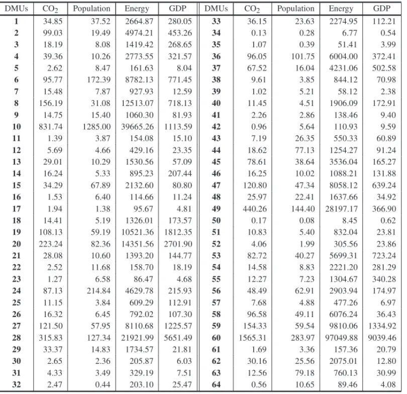
4 EXAMPLE
We use the same real data presented in Gomes & Lins (2008). In their case, DMUs are countries and the problem is to fairly distribute a single input, which is emission of CO2(carbon
equiv-alent ton3) considering three outputs: population (in million), energy (million BTU) and Gross Domestic Product (GDP, in billions of dollars).
Since this is a three outputs problem, the model formulation has two degrees of freedom,i.e., there are two eccentricities to be chosen. The 64 countries regarded as DMUs are:
(37) Netherlands (38) New Zealand (39) Nicaragua (40) Norway (41) Panama (42) Paraguay (43) Peru (44) Philippines (45) Poland (46) Portugal (47) Republic of Korea (48) Romania (49) Russian Federation (50) Seychelles (51) Slovakia (52) Slovenia (53) Spain (54) Sweden (55) Switzerland (56) Thailand (57) Turkmenistan (58) Ukraine (59) United Kingdom (60) United States (61) Uruguay (62) Uzbekistan (63) Vietnam (64) Zambia
Input and output real data values for each country are presented in Table 1.
Table 1– Inputs×Outputs from the example.
DMUs CO2 Population Energy GDP DMUs CO2 Population Energy GDP
1 34.85 37.52 2664.87 280.05 33 36.15 23.63 2274.95 112.21
2 99.03 19.49 4974.21 453.26 34 0.13 0.28 6.77 0.54
3 18.19 8.08 1419.42 268.65 35 1.07 0.39 51.41 3.99
4 39.36 10.26 2773.55 321.57 36 96.05 101.75 6004.00 372.41
5 2.62 8.47 161.63 8.04 37 67.52 16.04 4231.06 502.58
6 95.77 172.39 8782.13 771.45 38 9.61 3.85 844.12 70.98
7 15.48 7.87 927.93 12.59 39 1.02 5.21 58.12 2.38
8 156.19 31.08 12513.07 718.13 40 11.45 4.51 1906.09 172.91
9 14.75 15.40 1060.30 81.93 41 2.26 2.86 138.46 9.40
10 831.74 1285.00 39665.26 1113.59 42 0.96 5.64 110.93 9.59
11 1.39 3.87 154.08 15.10 43 7.19 26.35 550.33 60.89
12 5.69 4.66 429.16 23.35 44 18.62 77.13 1254.27 91.24
13 29.01 10.29 1530.56 57.09 45 78.61 38.64 3536.04 165.27
14 16.24 5.33 895.23 207.44 46 16.25 10.02 1088.21 131.88
15 34.29 67.89 2132.60 80.80 47 120.80 47.34 8058.12 639.24
16 1.53 6.40 114.66 11.24 48 25.97 22.41 1637.66 34.92
17 1.94 1.38 95.67 4.81 49 440.26 144.40 28197.17 366.90
18 14.41 5.19 1326.01 173.57 50 0.17 0.08 8.45 0.62
19 108.13 59.19 10521.36 1812.35 51 10.83 5.40 832.04 23.81
20 223.24 82.36 14351.56 2701.90 52 4.06 1.99 305.56 23.86
21 28.08 10.60 1393.20 144.77 53 82.72 40.27 5699.31 723.24
22 2.52 11.68 158.70 18.19 54 14.58 8.83 2221.20 281.29
23 1.27 6.58 86.47 4.68 55 12.27 7.23 1304.67 340.28
24 87.13 214.84 4629.78 215.93 56 48.49 62.91 2903.94 174.97
25 11.15 3.84 609.29 112.91 57 7.68 4.88 477.26 6.97
26 16.32 6.45 792.02 107.30 58 96.58 49.11 6076.24 36.43
27 121.50 57.95 8110.68 1225.57 59 154.33 59.54 9810.06 1334.92
28 315.83 127.34 21921.99 5651.49 60 1565.31 283.97 97049.88 9039.46
29 33.37 14.83 1734.57 21.81 61 1.69 3.36 157.36 20.79
30 2.65 2.36 205.87 6.03 62 30.16 25.56 2075.01 12.80
31 4.33 3.49 329.19 7.51 63 12.56 79.18 760.13 30.99
32 2.47 0.44 203.10 25.47 64 0.56 10.65 89.46 4.08
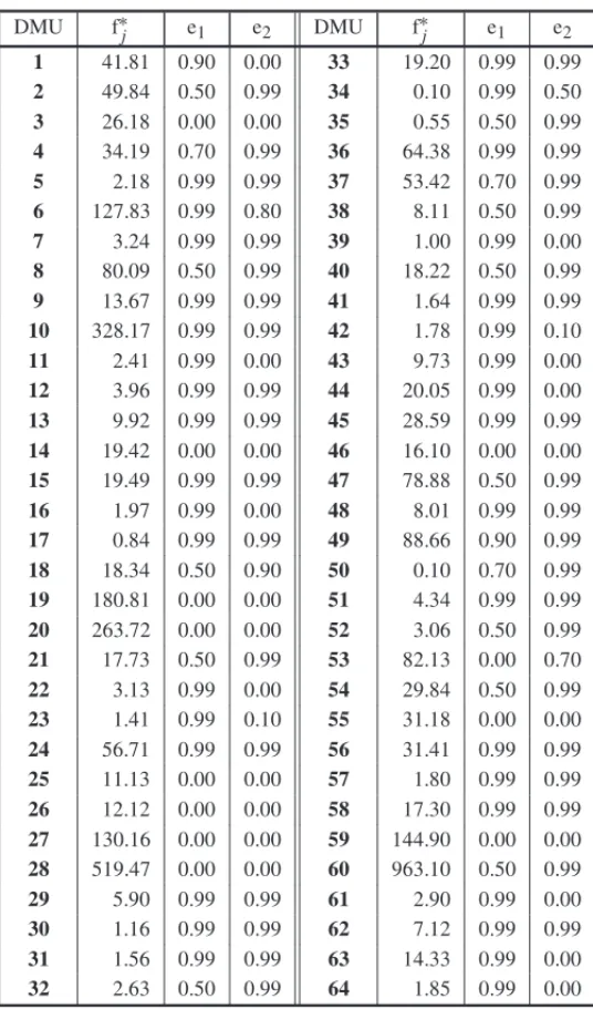
Table 2 shows the results obtained for the analysis carried out for each DMU.
Table 2– Local Analysis.
DMU f∗j e1 e2 DMU f∗j e1 e2
1 41.81 0.90 0.00 33 19.20 0.99 0.99
2 49.84 0.50 0.99 34 0.10 0.99 0.50
3 26.18 0.00 0.00 35 0.55 0.50 0.99
4 34.19 0.70 0.99 36 64.38 0.99 0.99
5 2.18 0.99 0.99 37 53.42 0.70 0.99
6 127.83 0.99 0.80 38 8.11 0.50 0.99
7 3.24 0.99 0.99 39 1.00 0.99 0.00
8 80.09 0.50 0.99 40 18.22 0.50 0.99
9 13.67 0.99 0.99 41 1.64 0.99 0.99
10 328.17 0.99 0.99 42 1.78 0.99 0.10
11 2.41 0.99 0.00 43 9.73 0.99 0.00
12 3.96 0.99 0.99 44 20.05 0.99 0.00
13 9.92 0.99 0.99 45 28.59 0.99 0.99
14 19.42 0.00 0.00 46 16.10 0.00 0.00
15 19.49 0.99 0.99 47 78.88 0.50 0.99
16 1.97 0.99 0.00 48 8.01 0.99 0.99
17 0.84 0.99 0.99 49 88.66 0.90 0.99
18 18.34 0.50 0.90 50 0.10 0.70 0.99
19 180.81 0.00 0.00 51 4.34 0.99 0.99
20 263.72 0.00 0.00 52 3.06 0.50 0.99
21 17.73 0.50 0.99 53 82.13 0.00 0.70
22 3.13 0.99 0.00 54 29.84 0.50 0.99
23 1.41 0.99 0.10 55 31.18 0.00 0.00
24 56.71 0.99 0.99 56 31.41 0.99 0.99
25 11.13 0.00 0.00 57 1.80 0.99 0.99
26 12.12 0.00 0.00 58 17.30 0.99 0.99
27 130.16 0.00 0.00 59 144.90 0.00 0.00 28 519.47 0.00 0.00 60 963.10 0.50 0.99
29 5.90 0.99 0.99 61 2.90 0.99 0.00
30 1.16 0.99 0.99 62 7.12 0.99 0.99
31 1.56 0.99 0.99 63 14.33 0.99 0.00
32 2.63 0.50 0.99 64 1.85 0.99 0.00
If we look at the result for DMU 1 presented in Tables 1 and 2 we conclude that Argentina’s current CO2 emission, which 34.85 carbon equivalent ton3has to climb to a minimum of 41.81
such that there will still be a solution for which global total CO2emission remains constant and
all DMUs (countries) are strong CCR efficient.
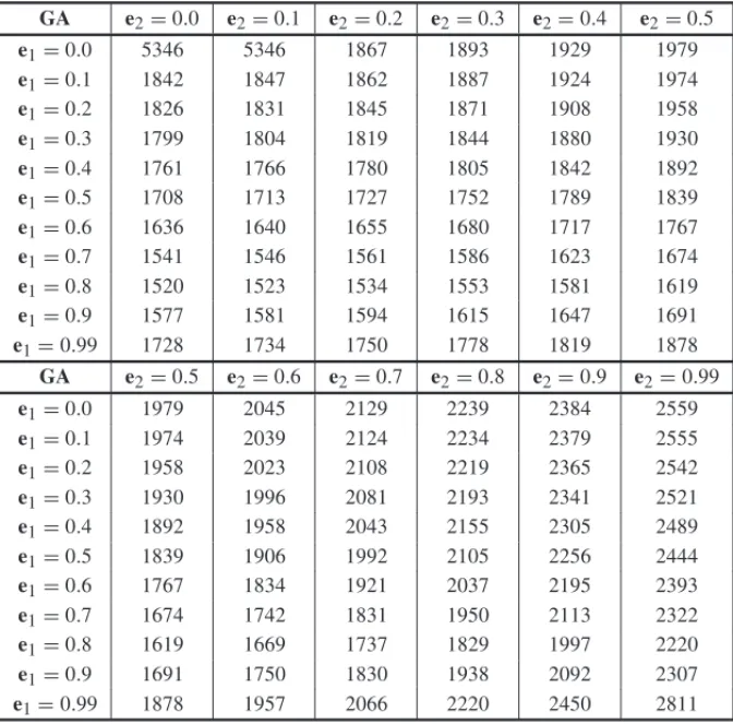
Table 3– Global Analysis.
GA e2=0.0 e2=0.1 e2=0.2 e2=0.3 e2=0.4 e2=0.5
e1=0.0 5346 5346 1867 1893 1929 1979
e1=0.1 1842 1847 1862 1887 1924 1974
e1=0.2 1826 1831 1845 1871 1908 1958
e1=0.3 1799 1804 1819 1844 1880 1930
e1=0.4 1761 1766 1780 1805 1842 1892
e1=0.5 1708 1713 1727 1752 1789 1839
e1=0.6 1636 1640 1655 1680 1717 1767
e1=0.7 1541 1546 1561 1586 1623 1674
e1=0.8 1520 1523 1534 1553 1581 1619
e1=0.9 1577 1581 1594 1615 1647 1691
e1=0.99 1728 1734 1750 1778 1819 1878
GA e2=0.5 e2=0.6 e2=0.7 e2=0.8 e2=0.9 e2=0.99
e1=0.0 1979 2045 2129 2239 2384 2559
e1=0.1 1974 2039 2124 2234 2379 2555
e1=0.2 1958 2023 2108 2219 2365 2542
e1=0.3 1930 1996 2081 2193 2341 2521
e1=0.4 1892 1958 2043 2155 2305 2489
e1=0.5 1839 1906 1992 2105 2256 2444
e1=0.6 1767 1834 1921 2037 2195 2393
e1=0.7 1674 1742 1831 1950 2113 2322
e1=0.8 1619 1669 1737 1829 1997 2220
e1=0.9 1691 1750 1830 1938 2092 2307
e1=0.99 1878 1957 2066 2220 2450 2811
As we can see from Table 3, the pair of eccentricities that minimizes total variability is the pair
(0.8,0.0).
For this study, all Local Analysis (Table 2) of the EFM model (Equation 2) were conducted using MSExcel. The Global Analysis (Table 3) was implemented on Matlab.
5 RESULTS AND CONCLUSION
In the LA, the largest differences between current and minimum possible values were observed for DMUs 10 (China), 28 (Japan), 49 (Russian Federation) and 60 (United States). For these Countries, the differences are, 503.57, 203.64, 351.60 and 602.23 ton3CO2found in
eccentric-ities (e1,e2) = (0.99,0.99), (0.00,0.00),(0.90,0.99)and(0.50,0.99), respectively. Among these countries, only DMU 28 (Japan) has a minimum value that is greater than its current value of emission.
possi-bilities ranging from 1520 ton3CO2(minimum) – found in the eccentricities values(e1,e2)= (0.80,0.00)– which represents 28% of the total F value, to 5346 ton3CO2(maximum). The
average was 1990 ton3CO2.
While observing both analysis results (LA and GA) the minimum value found on GA distribu-tion do not reveal any of the cases of LA distribudistribu-tion. However, the merit of this study is attained by indication of distributions with eccentricities values that occurs the solution of analyses LA and GA, according to each problem. The guidance while choosing one solution from many possibilities is now feasible, since it requires minimum data treatment. This is a relevant fact mainly due to the nature of input associated with many resources quantity.
REFERENCES
[1] AVELLAR JVG. 2004. Modelos DEA com soma constante de inputs/outputs. 106f. Dissertac¸˜ao (Mestrado em Engenharia Aeron´autica e Mecˆanica) – Instituto Tecnol´ogico de Aeron´autica. S˜ao Jos´e dos Campos. SP.
[2] AVELLARJVG, MILIONIAZ & RABELLOTN. 2005. Modelos DEA com vari´aveis limitadas ou soma constante.Pesquisa Operacional(Impresso), Rio de Janeiro, RJ,25(1): 135–150.
[3] AVELLARJVG, MILIONIAZ & RABELLOTN. 2007. Spherical Frontier DEA Model based on a constant sum of inputs.Journal od Operational Research Society,58: 1246–1251.
[4] AVELLARJVG. 2010. O modelo de fronteira elipsoidal: um modelo param´etrico para a distribuic¸˜ao de inputs de soma constante com controle nos pesos. 248f. Tese de Doutorado em Engenharia Aeron´autica e Mecˆanica – Instituto Tecnol´ogico de Aeron´autica. S˜ao Jos´e dos Campos. SP.
[5] AVELLARJVG, MILIONIAZ, RABELLOTN & SIMAO˜ HP. 2010. On the redistribution of existing inputs using the spherical frontier dea model.Pesquisa Operacional(Impresso),30: 1–16.
[6] BEASLEYJE. 2003. Allocating fixed costs and resources via data envelopment analysis.European Journal of Operational Research,147: 198–216.
[7] COOK WD & KRESS M. 1999. Characterizing an equitable allocation of shared costs: A DEA approach.European Journal of Operational Research,119: 652–661.
[8] GOMESEG & LINSMPE. 2008. Modelling undesirable outputs with zero sum gains data envelop-ment analysis models.Journal of the Operational Research Society,59: 616.
[9] GUEDESEC. 2007. Modelo de fronteira esf´erica ajustado: Alocando Input vi DEA param´etrico. Tese de Mestrado. Instituto Tecnol´ogico de Aeron´autica. S˜ao Jos´e dos Campos.
[10] GUEDES ECC, MILIONIAZ, AVELLAR JVG & SILVA RC. 2012. Adjusted spherical frontier model: allocating input via parametric DEA.Journal of the Operational Research Society,63: 406– 417.
[11] KASSAIS. 2002. Utilizac¸ ˜ao da An´alise por Envolt´oria de Dados (DEA) na an´alise de demonstra-c¸ ˜oes cont´abeis. 318f. Dissertademonstra-c¸˜ao (Doutorado em Contabilidade e Controladoria) – Universidade de S˜ao Paulo. S˜ao Paulo.
[13] LINSMPE, GOMESEG, SOARES DEMELOJCCB & SOARES DEMELOAJR. 2003. Olympic ranking based on a zero sum gains DEA model.European Journal of Operational Research,148: 312–322.
[14] MILIONIAZ, AVELLARJVG, GOMESEG & MELLOJCS. 2011a. An Ellipsoidal Frontier Model: allocating input via parametric DEA.European Journal of Operational Research,209: 113–121.
[15] MILIONIAZ, AVELLARJVG, RABELLOTN & FREITASGM. 2011b. Hyperbolic frontier model: a parametric DEA approach for the distribution of a total fixed input.Journal of the Operational Research Society,62: 1029–1037.
[16] SILVARC & MILIONIAZ. 2012. The Adjusted Spherical Frontier Model with Weight Restrictions. European Journal of Operational Research,220: 729–735.