TWO-STAGE INFERENCE IN EXPERIMENTAL DESIGN USING DEA: AN APPLICATION TO INTERCROPPING AND EVIDENCE FROM
RANDOMIZATION THEORY
Eliane Gonçalves Gomes* Geraldo da Silva e Souza
Brazilian Agricultural Research Corporation (Embrapa) Brasília – DF, Brazil
[email protected] [email protected]
Lúcio José Vivaldi
Statistics Department – University of Brasília (UNB) Brasília – DF, Brazil
* Corresponding author / autor para quem as correspondências devem ser encaminhadas
Recebido em 09/2007; aceito em 05/2008 após 1 revisão
Received September 2007; accepted August 2008 after one revision
Abstract
In this article we propose the use of Data Envelopment Analysis (DEA) measures of efficiency, under constant returns to scale and input equal to unity, in the analysis of multidimensional nonnegative responses in the design of experiments. The approach agrees with the standard Analysis of Variance (Covariance) for univariate responses and simplifies the statistical analysis in the multivariate case. The best treatments provided by the analysis optimize a combined output defined by shadow prices, which are the solutions of the DEA problem. The approach is particularly useful for the analysis of intercropping (crop mixtures) experiments. In this context we discuss two examples. To properly address the issue of correlation and non-normality of DEA measurements in different experimental plots we validate the results via Randomization Theory.
Keywords: experimental design; intercropping; data envelopment analysis.
Resumo
Neste artigo é proposto o uso de medidas de eficiência DEA, com retornos constantes à escala e input
unitário, na análise de respostas multidimensionais não negativas de ensaios experimentais. A abordagem proposta concorda com a Análise de Variância (Covariância) clássica para respostas unidimensionais e simplifica a análise estatística para o caso multidimensional. Os melhores tratamentos indicados pela análise otimizam um output combinado, definido por preços sombra, que são as soluções dos problemas lineares de DEA. A abordagem é particularmente útil na análise de experimentos consorciados (plantio simultâneo de mais de uma cultura agrícola). São aqui discutidos dois exemplos. Os resultados são validados via Teoria de Aleatorização, de modo a estudar apropriadamente as questões de correlação e não-normalidade das medidas DEA nas diferentes parcelas experimentais.
1. Introduction
In a designed experiment one measures a response, real valued or multidimensional, and carries out a regression analysis modeling the response as a function of qualitative effects (dummy variables) and possibly some quantitative variables (Montgomery, 2004; Hinkelman & Kempthorne, 2007a, 2007b; Ryan, 2007). These exogenous variables, under the control of the experimenter, are called contextual variables in the Data Envelopment Analysis (DEA) literature. Typical in this class of statistical procedures are the Analysis of Variance (only qualitative effects) and the Analysis of Covariance (qualitative and quantitative variables) models. Whenever the response is multidimensional the analysis is complex and the statistical findings are hard to interpret. For this reason in many applications one notices real efforts to reduce the dimensionality of the response vector to ease the statistical analysis.
Such is the case with intercropping experiments in agriculture, where a response, such as yield, is measured for each crop in a finite set of crops that are sown together in each experimental plot. The observation in each plot is therefore a vector of correlated yields since the crops compete for available resources. Typically, treatments applied to the experimental plots are to be compared on the basis of the yield vector. Indexes like total yield value, for example, transform the response vector to a nonnegative real variable, easing the statistical analysis relative to the use of multivariate analysis. The interest in intercropping is growing, as can be seen, for instance, in Blaser et al. (2006), Salgado et al. (2006), Bezerra Neto et al. (2007), Wang et al. (2007), Strydhorst et al. (2008).
Here we suggest a new approach to assess treatment differences in any designed experiment whose objective is to optimize response in some sense, where response is defined by a vector of yields. The proposal is to use DEA to generate a measure of efficiency to each experimental plot. This one-dimensional score can be analyzed by the classical statistical methods. DEA estimates of efficiency are flexible in the sense that they can be derived imposing or not a set of weights reflecting the importance of each component of the response vector (yield). If a designed experiment has a real valued nonnegative response, the DEA analysis as proposed here is equivalent to the usual statistical analysis carried out in Analysis of Variance (Covariance) models. In the multivariate case, besides simplifying the analysis, it endows the statistical conclusions with optimal properties in the sense that best treatments represent best yield practices relative to the complete set of treatments under analysis.
The exposition is divided into four sections. Section 2 defines the DEA efficiency measurements we deal with in the article. Section 3 shows the Analysis of Variance for two intercropping experiments using efficiency measurements (seen as scores or indexes) as responses to treatments. Section 4 is on validation of the statistical data analysis via Randomization Theory. Finally, Section 5 summarizes the main conclusions and the suggestions put forward in the article.
2. Data Envelopment Analysis
The efficiency of production of a DMU, in a typical DEA analysis, is defined by the ratio of a weighted average of the outputs by a weighted average of the inputs. These weights are shadow prices. They are distinct for outputs and inputs, and are determined by linear programming. For each DMU, the linear programming problem is set in such a way to maximize the efficiency ratio. Subjective or preconceived perceptions of the investigator about the relative importance of outputs and inputs may be included as restrictions in the linear programming problem.
There are two classical DEA models, the CCR (Charnes et al., 1978) and the BCC (Banker et al., 1984). The two models differ according to the convexity restriction imposed in the BCC DEA model. Two orientations are possible in any DEA model. One may look for maximal outputs given input levels, or one may look for minimal input utilization, given output levels.
In DEA modeling one has to define the DMUs, the production variables (inputs and outputs), the orientation and the model. In a designed experiment the DMUs are the experimental plots arranged in accordance with the layout of the experimental design. The nonnegative response vector of each experimental plot defines the output. Typically, treatments are applied to the experimental plots, like different management practices, and one is concerned with the assessment of treatment differences on the basis of the output vector. To measure the efficiency of each experimental plot we assume unitary inputs for all units. This idea is not strange in the DEA literature; see Lovell & Pastor (1999), De Koeijer et al. (2002), Leta et al. (2005). The model we consider is CCR with output orientation. We note that there are no issues of scale here, since the BCC solution for unit inputs coincide with the CCR solution, as stated and proved by Lovell & Pastor (1999). The assumption of unitary inputs is adequate for a designed experiment. It puts all experimental plots on the same basis for comparisons, and real differences in the response vector are therefore due to error control variables and to the influence of contextual variables, like treatments and other quantitative variables affecting the experimental plots and under the control of the investigator. Error control is typically achieved by design choice. In this context, using DEA scores as the response variable, the effects of contextual variables are to be assessed in a second stage, using a linear model where the classical assumptions (Steel et al., 1996) of the Analysis of Variance (Covariance) are postulated for the DEA efficiency measurements.
We now define the general DEA CCR model. Assume that each DMU (experimental plot) k, 1...
=
k n, is a production unit that uses m inputs (non-negatives, not all zeros) xik, i=1...r, to produce s outputs (non-negatives, not all zeros) yjk, j=1...s. The efficiency ho of
DMU o, with production values (x yo, o), is defined by the solution of the linear
programming problem
1
Min ,
= =
∑
ro i io
i
h v x subject to the restrictions
1
1
=
=
∑
s j joj
u y ,
1 1
0, 1,...,
= =
− ≤ =
∑
s j jk∑
r i ikj i
u y v x k n, uj, 0, vi≥ ,∀j i.
The quantities vi and ujare the shadow prices (weights) of inputs and outputs, respectively.
1 +
≤ ≤
j uj uj j
α β on the output shadow prices in the classic DEA models. In these restrictions, αj and βj are user-specified constants to reflect value judgements regarding the relative importance of outputs j and j+1, i.e., they are assigned by the decision-maker, here the investigator that is conducting the experiment. It is important to notice that the solutions for this problem (unitary input and multiple outputs) under constant returns and variable returns to scale still coincide.
We note here that is not necessary to assume an underlying frontier as a data generating process for the yield observations. We are concerned with the population of responses generated using empirical DEA for the experimental plots available for the experiment, classified according to the treatment arrangement laid out by the experimental design. Random allocation of treatment levels to experimental plots typically validate the statistical analysis resulting from the model induced by the design, which becomes the data generating model for the efficiency measurements. The main interest in the analysis is in the comparison of treatments, once these responses have been adjusted for the other quantitative covariates.
Responses may be defined as the DEA measurements themselves or by some monotonic transformation of these measurements, like ranks. However, it should be pointed out here that the design environment with yield responses does not violate typical production assumptions. It is not unreasonable to impose Assumptions A1, A4-A6 of Simar & Wilson (2007), as well as the separability condition A2 in the same article, since the covariates, in a typical design of experiments application, are measured without error and are under the control of the investigator. They are not correlated with the error term, which is the experimental error responsible for the variation among experimental units treated alike. They are unaffected by treatments and they are observed before the study (Kutner et al., 2005).
The dimension of the output vector relative to the size of the experiment is important in DEA. If the dimension is too large, one may have many efficient plots and this fact may obscure the study of treatments differences. The problem however does not exist for univariate yields and also for intercropping experiments, since the dimension of the output vector, in many applications, is two or three. The constant input helps to lessen this problem. It should be said here that a large dimension of the output vector would put hard problems also for a standard multivariate analysis of the design.
In Section 4 we continue with the discussion of the validity of the two-stage procedure involving DEA responses in a designed experiment.
3. Intercropping
Here we consider two experiments: a randomized complete block and a split-plot design over a factorial structure. It’s important to consider the two cases since they define different levels of complexity and may lead to different results regarding the validity of statistical tests in the corresponding Analysis of Variance (ANOVA).
3.1 Intercropping of Maize and Bean
are homogeneous. Each group is called a block and the number of experimental plots within each block may be the same or not. Treatments are randomly assigned to the experimental plots within each block. Blocking is used to control experimental error. The primary interest in the analysis is on treatment differences. Suppose one has n experimental plots, grouped in b blocks, and v treatments. Each block has kj experimental plots and each treatment appears
i
r times. One must have
∑
iv=1ri =∑
bj=1kj =n. If the experimental plot u has response yucorresponding (possibly) to xu, a vector of observations on controllable quantitative contextual variables or covariates, block j, and treatment i, one postulates
′
= + + + +
u i j u u
y µ α ρ β x ε , where µ is an overall mean, α =(α1…αv) is the vector of
treatment (parameter) effects, ρ=(ρ1…ρb) is the vector of block (parameter) effects, β′ is the parameter vector associated with the covariates, and the εu are iid random errors normally distributed with mean zero. Typically, the design matrix for the block design is singular but β′, and block and treatment contrasts, of the form p′α =0, p′1=0,
0, 1 0,
c′ρ= c′ = are estimable.
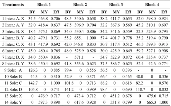
Table 1 shows responses and DEA efficiency measurements (Eff) for an intercropping experiment with maize and bean. The experiment was carried out at Embrapa (Brazilian Agricultural Research Corporation) and appears in Federer (1993). Four bean varieties (A, B, C e D) are intercropped with two maize varieties (X e Y). The crop combinations plus the sole crops, in a total of 14 levels, define the treatments here. The response is defined by the vector of yields of maize and beans measured by weight (Kg) per square meter. Sole crops show a zero in one of the yields.
Table 1 – Responses (bean yield – BY, maize yield – MY, and efficiency – Eff) for the intercropping of bean and maize in a randomized block experimental design.
Treatments Block 1 Block 2 Block 3 Block 4 BY MY Eff BY MY Eff BY MY Eff BY MY Eff
1 Inter.: A. X 34.5 463.8 0.706 48.5 340.6 0.658 38.2 411.7 0.653 52.0 598.0 0.924
2 Inter.: A. Y 32.0 418.4 0.637 47.5 396.9 0.704 32.2 367.6 0.569 45.2 310.1 0.607 3 Inter.: B. X 18.4 575.1 0.869 34.0 530.4 0.806 34.2 341.6 0.559 22.3 523.9 0.793 4 Inter.: B. Y 40.2 479.1 0.731 55.2 655. 1.000 57.4 401.7 0.778 35.2 519.4 0.790
5 Inter.: C. X 43.1 417.9 0.692 42.0 546.8 0.833 30.7 317.4 0.512 46.5 599.3 0.913 6 Inter.: C. Y 45.0 480.4 0.765 48.0 525.9 0.828 30.0 425.9 0.649 59.2 527.1 0.908 7 Inter.: D. X 34.0 550.4 0.836 - 571.1 - 54.7 522.9 0.872 60.4 335.4 0.737
8 Inter.: D. Y 38.6 450.4 0.692 41.8 353.6 0.623 37.5 386.7 0.625 52.4 42.6 0.774 9 Sole: A 126.3 0 0.885 79.4 0 0.556 56.5 0 0.396 - 0 - 10 Sole: B 44.3 0 0.310 52.9 0 0.371 66.4 0 0.465 48.0 0 0.336
11 Sole: C 142.7 0 1.000 101.8 0 0.713 88.2 0 0.618 82.2 0 0.576 12 Sole: D 105.8 0 0.741 141.2 0 0.989 98.4 0 0.690 118.7 0 0.832 13 Sole: X 0 476.9 0.717 0 473.4 0.712 0 451.2 0.678 0 475.6 0.715
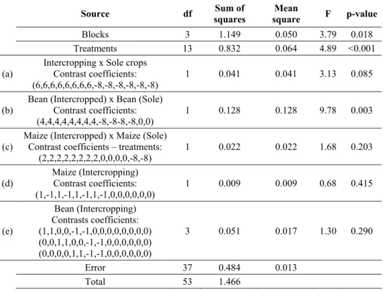
The DEA model should be run with 56 DMUs (14 treatments and 4 blocks), but there were missing data in two of them (treatment 7 – block 2, and treatment 9 – block 4). Thus, it was run with 54 DMUs, one single and constant input (equal to unit) and two outputs, bean yield (BY) and maize yield (MY). The analysis of variance of the experiment based on efficiency responses is shown in Table 2. The statistical analysis is carried out assuming the data generating process of the block design with DEA efficiency measurements as the observations on the dependent variable. Treatment contrasts of interest were also included in the analysis.
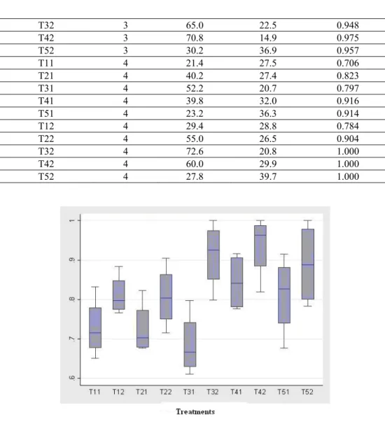
Efficiency seems to be the same for all variety combinations of maize and bean used in intercropping (rows (d) and (e), Table 2). Overall, there is no significant gain in efficiency of sole plots over intercropping (row (a), Table 2). Intercropped beans however are significantly more efficient than sole beans (row (b), Table 2). An interesting aspect of this intercropping experiment is that it shows a smaller risk for intercropped plots. Efficiency variation of intercropped plots is dominated by efficiency variation in sole plots. This remark is evident from Figure 1 where treatments 1-8 refer to intercropping and treatments 9-14 refer to sole crops (treatments 1-8 show less dispersion than treatments 9-14).
Efficiency responses belong to the interval (0.1], and treatment variances seem to be heterogeneous. In this context, one may perform an analysis of variance considering ranks as the response variable. The approach is non-parametric. We notice that this analysis leads to similar conclusions.
Table 2 – Analysis of variance for the intercropping of maize and bean. DEA efficiency is the response variable. Data generating process is defined by the randomized block design.
Source df Sum of squares
Mean
square F p-value
Blocks 3 1.149 0.050 3.79 0.018
Treatments 13 0.832 0.064 4.89 <0.001
(a)
Intercropping x Sole crops Contrast coefficients: (6,6,6,6,6,6,6,6,-8,-8,-8,-8,-8,-8)
1 0.041 0.041 3.13 0.085
(b)
Bean (Intercropped) x Bean (Sole) Contrast coefficients: (4,4,4,4,4,4,4,4,-8,-8-8,-8,0,0)
1 0.128 0.128 9.78 0.003
(c)
Maize (Intercropped) x Maize (Sole) Contrast coefficients – treatments:
(2,2,2,2,2,2,2,2,0,0,0,0,-8,-8)
1 0.022 0.022 1.68 0.203
(d)
Maize (Intercropping) Contrast coefficients: (1,-1,1,-1,1,-1,1,-1,0,0,0,0,0,0)
1 0.009 0.009 0.68 0.415
(e)
Bean (Intercropping) Contrasts coefficients: (1,1,0,0,-1,-1,0,0,0,0,0,0,0,0) (0,0,1,1,0,0,-1,-1,0,0,0,0,0,0) (0,0,0,0,1,1,-1,-1,0,0,0,0,0,0)
3 0.051 0.017 1.30 0.290
Error 37 0.484 0.013
Figure 1 – Box plots of treatments. Intercropping of maize and bean.
3.2 Intercropping of Groundnut and Maize
The second experiment we consider is the intercropping of groundnut and maize in a randomized block design laid out as a split plot. The underlying principle of the split plot is this: the levels of a factor A (treatment A) are applied to the experimental plots arranged as in the randomized block design. Each experimental plot is then divided into subplots to which the levels of a second factor B (treatment B) are applied. In this context each experimental plot becomes a block for factor B. The randomization is carried out in two stages. First the levels of A are randomized over the (whole) experimental plots. Then the levels of B are randomized over the subplots. The reference is Steel et al. (1996).
The data generating process for the split plot assuming the randomized block design is as follows. Let yijk = +µ ρ αi+ j+γij+δk +
( )
αδ jk+εijk denote the observation in the ith blockof a randomized (complete) block design, on the jth level of factor A with the kth level of factor B. Here i=1…r blocks, j=1...a levels of factor A, and k=1...b levels of factor B. The error components γij and εijk are normally and independently distributed about zero
means, with σγ2 being the common variance of the γij and σε2 the variance of the εijk. The
error component γij is the whole plot random error (Error A) and
ε
ijk is the subplot random error (Error B). The parameters µ ρ α δ, i, j, k,( )
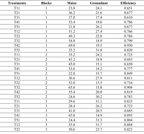
αδ jk represent an overall mean, blockTable 3 shows production and efficiency data for an intercropping experiment involving maize and groundnuts. Response for each crop is measured in tons/acre. The experiment was carried out in the substation of Morwa, in Samuru, Nigeria. It is described in Carvalho (1988). The whole experimental plot treatment levels are defined by factor A with 5 levels, which are repeated in 4 blocks. The levels of A are defined by the plant densities (maize: groundnut) 1:3, 1:2, 2:3, 4:9, and 1:6. The subplot treatment, factor B, comprises two levels of nitrogen treated as qualitative. We denote by 1-5 the plant densities and by 1-2 the nitrogen levels.
Figure 2 shows clearly an increase in efficiency due to nitrogen level 2 independently of the plant density (treatments Tx2 have higher response that treatments Tx1). It is also evident the dominance of plant density 4. A non-parametric analysis of variance is shown in Table 4. The response considered for this analysis is rank of efficiency. The ranks are assumed to follow the data generating process of the split plot with the randomized block design. The interaction A*B is significant.
Table 3 – Responses (maize yield, groundnut yield, efficiency) for a factorial design laid out as a randomized block design with a split plot structure. The first index in treatment combination Tij refers to a level of Factor A (plant density) and the second to a level of Factor B (nitrogen level).
Treatments Blocks Maize Groundnut Efficiency
T11 1 23.8 24.1 0.651
T21 1 36.2 21.6 0.677
T31 1 37.8 17.4 0.610
T41 1 53.4 19.0 0.786
T51 1 21.0 26.2 0.677
T12 1 31.2 27.4 0.766
T22 1 49.2 22.0 0.786
T32 1 54.8 18.9 0.799
T42 1 69.0 19.5 0.950
T52 1 25.2 31.8 0.820
T11 2 35.2 24.2 0.725
T21 2 43.2 18.8 0.683
T31 2 45.0 15.1 0.650
T41 2 53.6 18.2 0.777
T51 2 22.8 33.7 0.849
T12 2 36.6 27.9 0.811
T22 2 52.0 13.5 0.716
T32 2 65.6 15.8 0.904
T42 2 55.4 20.0 0.819
T52 2 24.6 30.2 0.783
T11 3 29.6 31.1 0.833
T21 3 28.4 26.2 0.723
T31 3 41.0 20.5 0.685
T41 3 65.0 14.9 0.895
T51 3 24.4 31.3 0.804
T12 3 35.8 31.7 0.884
T32 3 65.0 22.5 0.948
T42 3 70.8 14.9 0.975
T52 3 30.2 36.9 0.957
T11 4 21.4 27.5 0.706
T21 4 40.2 27.4 0.823
T31 4 52.2 20.7 0.797
T41 4 39.8 32.0 0.916
T51 4 23.2 36.3 0.914
T12 4 29.4 28.8 0.784
T22 4 55.0 26.5 0.904
T32 4 72.6 20.8 1.000
T42 4 60.0 29.9 1.000
T52 4 27.8 39.7 1.000
Figure 2 – Box plots of treatments. Intercropping of groundnut and maize.
Table 4 – Analysis of variance table for ranks of efficiencies of experimental units. Intercropping of groundnut and maize in a split plot with a randomized block design.
Source df Sum of squares Mean square F p-value
Blocks 3 1499.20 499.73 8.20 0.003
A 4 990.25 247.56 4.06 0.026
Error A 12 731.55 60.96 - -
B 1 1276.90 1276.90 43.07 < 0.0001
A*B 4 385.35 96.34 3.25 0.042
Error B 15 444.75 29.65 - -
Table 5 provides information on the average efficiency rank per treatment (means over efficiency ranks for the intercropping of maize and groundnut). Comparison of two A means, at the same or different levels of B, involve both main effect A and interaction A*B. The two error component are involved, the whole plot error and the subplot error. The variance of the
difference is given by ⎛ ⎞⎜ ⎟2
(
2+ 2)
⎝ ⎠r σγ σε . An unbiased estimate of
(
)
2+ 2
γ ε
σ σ is given by
a b
MSE ( 1) MSE
b + −b
, where MSEa and MSEb are the mean square errors for errors A and
B, respectively (Milliken & Johnson, 1984; Steel et al., 1996). The sampling distribution associated with this unbiased estimate is not square but a linear combination of chi-square distributions. There is not an exact least significant difference for the comparison of two A means. Using the method of moments an approximate value can be computed. The procedure is similar to the one used when the means of two populations with distinct variances are compared. Following Milliken & Johnson (1984, p.303), the least significant
difference for comparing any two A means at the 5% level is 60.96 29.65 4
∗ +
=
lsd t . In this
expression
12 15
0.975 60.96 0.975 29.65
60.96 29.65
∗= × + ×
+
t t
t , where r
tα is the quantile of order α of the
Student distribution with r degrees of freedom. Thus, lsd=10.30.
Table 5 – Treatment means of efficiency ranks for the intercropping of maize and groundnut.
Treatment Mean
T11 12.00 T21 11.50 T31 07.00 T41 23.00 T51 20.75 T12 19.00 T22 20.00 T32 30.50 T42 33.25 T52 28.00
We see that the visual impression of Figure 2 is confirmed. Responses associated with nitrogen level 2 are dominant. Treatment combination 42 has the highest efficiency. However it does not differ significantly (5%) from T32 or T52.
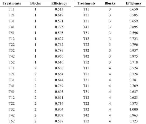
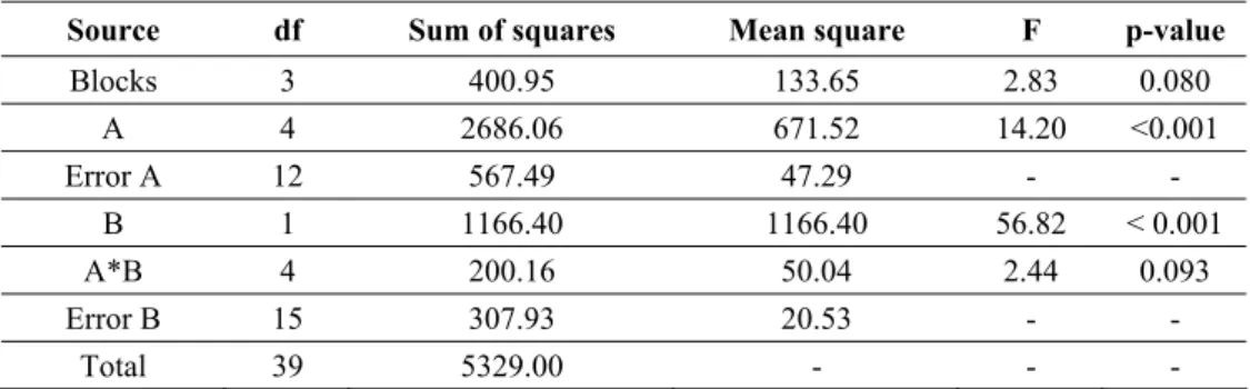
If the investigator feels that maize is more important than groundnut, this perception can be incorporated in the analysis using DEA models with Assurance Region weights restrictions approach (umaize ugroundnut ≥1), as discussed in Section 2. It leads to the data in Table 6 and the analysis shown in Table 7 when the responses are ranks. The interaction A*B is no longer significant at the 5% level. At this level of significance the least significant difference for A comparisons is 7.49. The A means are 12.13, 20.62, 26.00, 36.63 and 10.93, respectively. The best density is level 4, which is superior significantly to densities 1, 2, and 5 and marginally to density 3. The least significant difference for comparison of nitrogen levels is 3.05 and the observed mean difference is 10.8. Level 2 is superior as before.
Table 6 – Responses (efficiency) for a factorial design laid out as a randomized block design with a split plot structure. The first index in treatment combination Tij refers to a level of Factor A
(plant density) and the second to a level of Factor B (nitrogen level). Perception groundnut ≤ maize incorporated.
Treatments Blocks Efficiency Treatments Blocks Efficiency
T11 1 0.513 T11 3 0.650
T21 1 0.619 T21 3 0.585
T31 1 0.591 T31 3 0.659
T41 1 0.775 T41 3 0.895
T51 1 0.505 T51 3 0.596
T12 1 0.627 T12 3 0.723
T22 1 0.762 T22 3 0.796
T32 1 0.789 T32 3 0.937
T42 1 0.950 T42 3 0.975
T52 1 0.610 T52 3 0.718
T11 2 0.636 T11 4 0.524
T21 2 0.664 T21 4 0.724
T31 2 0.644 T31 4 0.781
T41 2 0.769 T41 4 0.769
T51 2 0.605 T51 4 0.637
T12 2 0.691 T12 4 0.623
T22 2 0.716 T22 4 0.873
T32 2 0.904 T32 4 1.000
T42 2 0.807 T42 4 0.963
Table 7 – Analysis of variance table for ranks of efficiencies of experimental plots. Intercropping of groundnut and maize in a split plot with a randomized block design.
Perception groundnut ≤ maize incorporated.
Source df Sum of squares Mean square F p-value
Blocks 3 400.95 133.65 2.83 0.080
A 4 2686.06 671.52 14.20 <0.001
Error A 12 567.49 47.29 - -
B 1 1166.40 1166.40 56.82 < 0.001
A*B 4 200.16 50.04 2.44 0.093
Error B 15 307.93 20.53 - -
Total 39 5329.00 - - -
4. Validation
The assumptions behind the statistical analysis carried in both examples of the previous section are strong and can be questioned. Typically, errors are uncorrelated and normally distributed. DEA efficiency responses cannot be normally distributed. The use of DEA efficiency measures as a response variable in regression models has been questioned recently in the econometric literature. See Simar & Wilson (2007). Besides normality, another issue in this discussion is that the analysis is carried out in two stages and in the first stage a correlation between experimental units is induced by the computation (and the definition) of the response variable and the potential association of covariates with the error term. In this context, one loses the distributional properties of the least squares estimators. For designed experiments however, the analysis of variance is known to be robust against many departures from the linear models defining the data generating process. Including non-normality and correlation among the experimental plots responses. On the other hand, covariates are not considered random in a designed experiment.
The random allocation of treatments to the experimental plots is the key feature that validates the statistical analysis besides allowing a method to verify if the significance levels induced by the normal theory are correct or not. Fisher (1925) extensively promoted this experimental process. A good discussion on this theory may also be seen in Hinkelman & Kempthorne (2007a, 2007b) and Kutner et al. (2005).
Based on the robustness of the statistical analysis of designed experiments, we should stress once again that the issues of correlation and non-normality are of secondary importance in many applications. For example, with unitary inputs and a single response, the measure of efficiency proposed here amounts simply to divide the values of the response by its sample maximum. Since t and F statistics are invariant by scale transformations, the statistical results are unaffected by the two-stage process. The situation with multiple outputs is more complex. Our experience is that the correlation is not sufficiently strong to invalidate the analysis. In a previous study (Souza et al., 2007), we did not find that the correlation was significant.
For a complete randomized block design with r blocks and v treatments there are
( )
v!r possible assignments of treatments to experimental plots. Consider the F statistics used to test equality of treatment effects. Each treatment assignment generates a value for F. The collection of these F values defines the distribution of F under randomization. Typically the number of possible treatment allocations is large and one works with a random sample from this population. Here we use 10,000 random allocations, which will generate 10,000 F values. We note that in these simulations the DEA responses are fixed in each experimental plot. Only the treatment allocations change.For the split plot arranged in r blocks with a levels of factor A applied to main plots and b levels of factor B applied to the subplots, there will be
(
a b! !)
r possible treatment allocations to the experimental plots. The statistics of main concern here are the F test statistics for the effects A, B and the interaction A*B. Here we also use 10,000 random allocations.For a more complete discussion in randomization test see, for instance, Edgington & Onghena (2007).
4.1 Intercropping of Maize and Bean
We used SAS v9.1.3 to program a Macro to generate 10,000 values of the F statistic used for testing equality of treatment effects under normal theory. The SAS procedures used were PROC PLAN and PROC GLM. Table 8 shows the quantiles of the two distributions involved.
The quantiles of the two distributions are close. The analyses with normal theory and with randomization are coincident. The empirical p-value does not point to any significant discrepancy.
Table 8 – Comparison of quantiles. Intercropping of maize and bean. Randomized block design.
Quantile (%) F (Normal) F (Randomization)
90 1.71 1.71
95 2.00 2.03
99 2.66 2.76
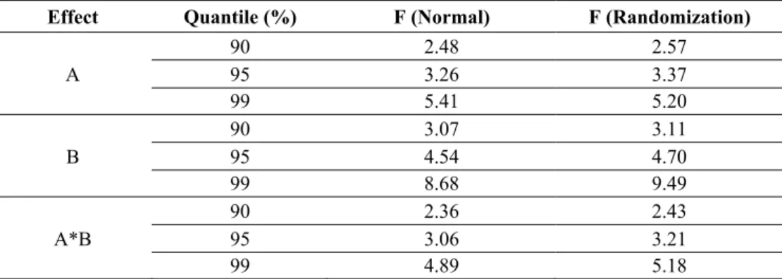
4.2 Intercropping of Groundnut and Maize
Here, also, a macro SAS was developed to generate values of the three F statistics associated with the effects A, B, and A*B. Table 9 shows the quantiles of the distributions of these test statistics under normality and under randomization.
Table 9 – Quantiles of the distributions under normality and randomization. Intercropping of groundnut and maize. Randomized block design with split-plot.
Effect Quantile (%) F (Normal) F (Randomization)
90 2.48 2.57
A 95 3.26 3.37
99 5.41 5.20
90 3.07 3.11
B 95 4.54 4.70
99 8.68 9.49
90 2.36 2.43
A*B 95 3.06 3.21
99 4.89 5.18
5. Conclusions
We propose the use of DEA output oriented efficiency measurements, under constant returns to scale, assuming a unitary input, as the response of each experimental plot in a designed experiment whenever the output vector is defined by non-negative yields. The technique consists in applying the normal theory or non-parametric (rank) methods to the efficiency measurements. This proposed approach, with the validation test, has never been used before in intercropping experiments.
The analysis coincides with the classical analysis of variance when yield is univariate, since the analysis of variance computations are invariant under scale transformations. The use of DEA has a strong appeal in the analysis of intercropping experiments were, typically, one is looking for the most efficient combination of two or more cultures.
In this context, we illustrated the efficiency analysis using two randomized block designs. One of them with the structure of a split plot. The intercropping considered were maize and bean for the randomized block design, and groundnut and maize for the split plot. In both cases the statistical analysis with efficiency scores is simpler and more objective than that based on the bivariate normal distribution. The classical analysis of variance for the efficiency scores in the two instances was validated via Randomization Theory, reinforcing its usefulness in this kind of application.
References
(1) Banker, R.D.; Charnes, A. & Cooper, W.W. (1984). Some models for estimating technical scale inefficiencies in data envelopment analysis. Management Science, 30(9), 1078-1092.
(2) Bezerra Neto, F.; Gomes, E.G.; Nunes, M.V.R. & Barros Junior, A.P. (2007). Análise multidimensional de consórcios cenoura-alface sob diferentes combinações de densidades populacionais. Pesquisa Agropecuária Brasileira, 42(12), 1697-1704.
(3) Blaser, B.C.; Gibson, L.R.; Singer, J.W. & Jannink, J.L. (2006). Optimizing seeding rates for winter cereal grains and frost-seeded red clover intercrops. Agronomy Journal,
(4) Carvalho, J.R.P. (1988). Bivariate analysis in intercropping with two levels of error variation. 245f. Thesis (Doctor of Philosophy) – Department of Applied Statistics. University of Reading, Reading.
(5) Charnes, A.; Cooper, W.W. & Rhodes, E. (1978). Measuring the efficiency of decision-making units. European Journal of Operational Research, 2, 429-444.
(6) De Koeijer, T.J.; Wossink, G.A.A.; Struik, P.C. & Renkema, J.A. (2002). Measuring agricultural sustainability in terms of efficiency: the case of Dutch sugar beet growers. Journal of Environmental Management, 66, 9-17.
(7) Edgington, E. & Onghena, P. (2007). Randomization Tests. 4th edition. Chapman & Hall, New York.
(8) Federer, T.W. (1993). Statistical design and analysis for intercropping experiments: two crops. Springer, New York.
(9) Fisher, R.A. (1925). Statistical methods for research workers. Oliver & Boyd, Edinburgh.
(10) Hinkelman, K. & Kempthorne, O. (2007a). Design and Analysis of Experiments: Introduction to Experimental Design. Wiley, New York, Vol. 1.
(11) Hinkelman, K. & Kempthorne, O. (2007b). Design and Analysis of Experiments: Advanced Experimental Design. Wiley, New York, Vol. 2.
(12) Kutner, M.H.; Nachtsheim, C.J.; Neter, J. & Li, W. (2005). Applied Linear Statistical Models. 5th ed. McGraw-Hill – Irwin, New York.
(13) Leta, F.R.; Soares de Mello, J.C.C.B.; Gomes, E.G. & Angulo Meza, L. (2005). Métodos de melhora de ordenação em DEA aplicados à avaliação estática de tornos mecânicos. Investigação Operacional, 25(2), 229-242.
(14) Lovell, C.A.K. & Pastor, J.T. (1999). Radial DEA models without inputs or without outputs. European Journal of Operational Research, 118(1), 46-51.
(15) Milliken, G.A. & Johnson, D.E. (1984). Analysis of Messy Data. Van Nostrand, New York.
(16) Montgomery, D.C. (2004). Design and Analysis of Experiments. 6th edition. Wiley, New York.
(17) Ryan, T.P. (2007). Modern Experimental Design. Wiley, New York.
(18) Salgado, A.S.; Guerra, J.G.M.; Almeida, D.L.; Ribeiro, R.L.D.; Espindola, J.A.A. & Salgado, J.A.A. (2006). Consórcios alface-cenoura e alface-rabanete sob manejo orgânico. Pesquisa Agropecuária Brasileira, 41(7), 1141-1147.
(19) Simar, L. & Wilson, P.W. (2007). Estimation and inference in two-stage, semiparametric models of production processes. Journal of Econometrics, 136(1), 31-64.
(20) Souza, G.S.; Gomes, E.G.; Magalhães, M.C. & Avila, A.F.D. (2007). Economic efficiency of Embrapa s research centers and the influence of contextual variables. Pesquisa Operacional, 27, 15-26.
(22) Steel, R.G.D.; Torrie, J.H. & Dickey, D.A. (1996). Principles and Procedures of Statistics: A Biometrical Approach. McGraw-Hill, New York.
(23) Thanassoulis, E.; Portela, M.C. & Allen, R. (2004). Incorporating value judgments in DEA. In: Handbook on Data Envelopment Analysis [edited by W.W. Cooper, L.M. Seiford & J. Zhu], Springer, New York, 99-138.