FORTRAN SUBROUTINES FOR NETWORK FLOW OPTIMIZATION USING AN INTERIOR POINT ALGORITHM
L. F. Portugal
Dep. de Ciências da Terra – Universidade de Coimbra Coimbra – Portugal
M. G. C. Resende*
Internet and Network Systems Research Center AT&T Labs Research
Florham Park – NJ, USA [email protected]
G. Veiga HTF Software
Rio de Janeiro – RJ, Brazil [email protected]
J. Patrício
Instituto Politécnico de Tomar – Tomar – Portugal e Instituto de Telecomunicações – Polo de Coimbra – Portugal [email protected]
J. J. Júdice
Dep. de Matemática – Univ. de Coimbra – Coimbra e Instituto de Telecomunicações – Polo de Coimbra – Portugal [email protected]
* Corresponding author / autor para quem as correspondências devem ser encaminhadas
Recebido em 01/2007; aceito em 04/2008 Received January 2007; accepted April 2008
Abstract
We describe Fortran subroutines for network flow optimization using an interior point network flow algorithm, that, together with a Fortran language driver, make up PDNET. The algorithm is described in detail and its implementation is outlined. Usage of the package is described and some computational experiments are reported. Source code for the software can be downloaded at http://www.research.att.com/~mgcr/pdnet.
Keywords: optimization; network flow problems; interior point method; conjugate gradient
method; FORTRAN subroutines.
Resumo
É apresentado o sistema PDNET, um conjunto de subrotinas em Fortran para a otimização de fluxos lineares em redes utilizando um algoritmo de pontos interiores. O algoritmo e a sua implementação são descritos com algum detalhe. A utilização do sistema é explicada e são apresentados alguns resultados computacionais. O código fonte está disponível em http://www.research.att.com/~mgcr/pdnet.
Palavras-chave: otimização; problemas de fluxo em rede; método de ponto interior; método
1. Introduction
Given a directed graph G=( , )V E , where V is a set of m vertices and E a set of n edges, let ( , )i j denote a directed edge from vertex i to vertex j. The minimum cost network flow problem can be formulated as
( , ) min ij ij
i j
c x ∈
∑
E subject to
(1)
( , ) ( , )
,
ij ji i
i j j i
x x b i
∈ ∈
− = ∈
∑
∑
E E
V
(2) lij≤xij ≤uij, ( , )i j ∈E,
where xij denotes the flow on edge ( , )i j and cij is the cost of passing one unit of flow on edge ( , )i j . For each vertex i∈V, bi denotes the flow produced or consumed at vertex i. If
0 i
b > , vertex bi is a source. If bi<0, vertex i is a sink. Otherwise (bi=0), vertex i is a transshipment vertex.
For each edge ( , )i j ∈E, lij (uij) denotes the lower (upper) bound on flow on edge ( , )i j . Most often, the problem data are assumed to be integer. In matrix notation, the above network flow problem can be formulated as a primal linear program of the form
(3) min {c x Ax| =b x; + =s u x s; , ≥0}
where c is a m n× vector whose elements are cij, A is the m n× vertex-edge incidence
matrix of the graph G=( , )V E , i.e. for each edge ( , )i j in E there is an associated column in matrix A with exactly two nonzero entries: an entry 1 in row i and an entry −1 in row j;
b, x, and u are defined as above, and s is an n-dimensional vector of upper bound slacks. Furthermore, an appropriate variable change allows us to assume that the lower bounds l are zero, without loss of generality. The dual of (3) is
(4) max {b y u w A y− | − + =w z c z w; , ≥0}
where y is the m-dimensional vector of dual variables and w and z are n-dimensional vectors of dual slacks.
If graph G is disconnected and has p connected components, there are exactly p redundant flow conservation constraints, which are sometimes removed from the problem formulation. Without loss of generality, we rule out trivially infeasible problems by assuming
0, 1, , k
j j
b k p
∈
= = …
∑
V
,
where Vk is the set of vertices for the k-th component of G.
If it is required that the flow xij be integer, (2) is replaced with
, integer, ( , ) ij ij ij ij
In the description of the algorithm, we assume without loss of generality, that lij =0 for all ( , )i j ∈E and that c≠0. A simple change of variables is done in the subroutines to transform the original problem into an equivalent one with lij =0 for all ( , )i j ∈E. The flow is transformed back to the original problem upon termination. The case where c=0 is a simple feasibility problem, and is handled by solving a maximum flow problem [1].
Before concluding this introduction, we present some notation and outline the remainder of the paper. We denote the i-th column of A by Ai, the i-th row of A by Aii and a submatrix of A formed by columns with indices in set S by AS. Let x∈Rn. We denote by
X the n n× diagonal matrix having the elements of x in the diagonal. The Euclidean or 2-norm is denoted by ·‖‖.
This paper describes Fortran subroutines used in an implementation of PDNET, an interior point network flow method introduced in Portugal, Resende, Veiga & Júdice [12]. The paper is organized as follows. In Section 2 we review the truncated infeasible-primal feasible-dual interior point method for linear programming. The implementation of this algorithm to handle network flow problems is described in Section 3. Section 4 describes the subroutines and their usage. Computational results, comparing PDNET with the network optimizer in CPLEX 10, are reported in Section 5. Concluding remarks are made in Section 6.
2. Truncated primal-infeasible dual-feasible interior point algorithm
In this section, we recall the interior point algorithm implemented in PDNET. Let
{( , , , , )x y s w z n m n n n+ + + + :x 0,s 0,w 0,z 0}
+= ∈R > > > >
Q
{( , , , , )x y s w z :x s u A y, w z c}
+= ∈ + + = − + =
S Q .
The truncated primal-infeasible dual-feasible interior point (TPIDF) algorithm [12] starts with any solution (x0,y s w z0, 0, 0, 0)∈S+. At iteration k, the Newton direction
(∆xk,∆yk,∆sk,∆wk,∆zk) is obtained as the solution of the linear system of equations
(5)
, 0,
0,
, ,
k k k
k k
k k k
k k k k k k
k
k k k k k k
k
A x b Ax r
x s
A y w z
Z x X z e X Z e
W s S w e W S e
µ µ
∆ = − +
∆ + ∆ =
∆ − ∆ + ∆ =
∆ + ⎧
∆ = −
∆ + ∆ =
⎪ ⎪ ⎪ ⎨
− ⎪
⎪ ⎪ ⎩
where e is a vector of ones of appropriate order, rk is such that
(6) 0 , 0 0 1
k k
r ≤β Ax −b ≤β <β
‖ ‖ ‖ ‖ ,
with β =1 0.1, and
(7) 1( ) ( )
2
k k k k
k
x z w s
n
Primal and dual steps are taken in the direction (∆xk,∆yk,∆sk,∆wk,∆zk) to compute new iterates according to
(8) 1 1 1 1 1 , , , , ,
k k k
p
k k k
p
k k k
d
k k k
d
k k k
d
x x x
s s s
y y y
w w w
z z z
α α α α α + + + + + = + ∆ = + ∆ = + ∆ = + ∆ = + ∆
where αp and αd are step-sizes in the primal and dual spaces, respectively, and are given by
(9) max{ : 0, 0},
max{ : 0, 0},
k k k k
p p
k k k k
d d
x x s s
w w z z
α α α α
α α α α
= + ∆ ≥ + ∆ ≥
= + ∆ ≥ + ∆ ≥
where p= d =0.9995.
The solution of the linear system (5) is obtained in two steps. First, we compute the ∆yk
component of the direction as the solution of the system of normal equations (10) AΘkA ∆yk = − ΘA k(µk(Xk)−1e−µk(Sk)−1e c− +A yk) (+ −b Axk), where Θk is given by
(11) Θ =k (Zk(Xk)−1+Wk(Sk) )− −1 1. The remaining components of the direction are then recovered by
(12) 1 1 1 1 1 1 ( ( ) ( ) ), , ( ) ( ) , ( ) ( ) .
k k k k k k k
k k
k k
k k k k k k
k
k k k k k k
k
x A y X e S e c A y
s x
z z X e Z X x
w w S e W S s
µ µ µ µ − − − − − −
∆ = Θ ∆ + Θ − − +
∆ = − ∆
∆ = − + − ∆
∆ = − + − ∆
3. Implementation
We discuss how the truncated primal-infeasible dual-feasible algorithm can be used for solving network flow problems. For ease of discussion, we assume, without loss of generality, that the graph G is connected. However, disconnected graphs are handled by PDNET.
3.1 Computing the Newton direction
Since the exact solution of (10) can be computationally expensive, a preconditioned conjugate gradient (PCG) algorithm is used to compute approximately an interior point search direction at each iteration. The PCG solves the linear system
(13) M−1(AΘkA )∆ =yk M b−1 , where M is a positive definite matrix and Θk is given by (11), and
1 1
( ( ) ( ) ) ( )
k k k k k
k k
The aim is to make the preconditioned matrix
(14) M−1(AΘkA )
less ill-conditioned than AΘkA , and improve the efficiency of the conjugate gradient algorithm by reducing the number of iterations it takes to find a feasible direction.
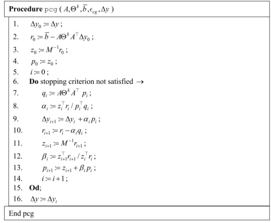
Pseudo-code for the preconditioned conjugate gradient algorithm implemented in PDNET is presented in Figure 1. The matrix-vector multiplications in line 7 are of the form AΘkA pi, and can be carried out without forming AΘkA explicitly. PDNET uses as its initial direction
0
y
∆ the direction ∆y produced in the previous call to the conjugate gradient algorithm, i.e. during the previous interior point iteration. The first time pcg is called, we assume
0 (0, , 0)
y
∆ = … .
The preconditioned residual is computed in lines 3 and 11 when the system of linear equations
(15) Mzi+1=ri+1,
is solved. PDNET uses primal-dual variants of the diagonal and spanning tree preconditioners described in [15,16].
Procedurepcg (A,Θk, ,b εcg,∆y) 1. ∆y0:= ∆y;
2. r0:= − Θb A kA ∆y0; 3. z0: M r10
−
= ; 4. p0:=z0; 5. i: 0= ;
6. Do stopping criterion not satisfied → 7. qi:= ΘA kA pi;
8. αi:=z r p qi i/ i i; 9. ∆yi+1:= ∆ +yi αipi; 10. ri+1:= −ri αi iq ; 11. zi1: M r1i1
−
+ = + ;
12. βi:=z ri+ +1i1/z ri i; 13. pi+1:=zi+1+βipi; 14. i:= +i 1;
15. Od; 16. ∆ = ∆y: yi
End pcg
The diagonal preconditioner, M =diag(AΘkA ), can be constructed in O n( ) operations, and makes the computation of the preconditioned residual of the conjugate gradient possible with O m( ) divisions. This preconditioner has been shown to be effective during the initial interior point iterations [11,14,15,16,18].
In the spanning tree preconditioner [16], one identifies a maximal spanning tree of the graph
G, using as weights the diagonal elements of the current scaling matrix, k
w= Θ e,
where e is a unit n-vector. An exact maximal spanning tree is computed with the Fibonacci heap variant of Prim’s algorithm [13], as described in [1]. At the k-th interior point iteration, let Tk ={ ,t1…, }tq be the indices of the edges of the maximal spanning tree. The spanning tree preconditioner is
k k k k
M=AT ΘT AT ,
where
1
diag( , , )
k q
k k k
t t
Θ = Θ … Θ
T .
For simplicity of notation, we include in ATk the linear dependent rows corresponding to the redundant flow conservation constraints. At each conjugate gradient iteration, the preconditioned residual system
1 1 i i
Mz+ =r+
is solved with the variables corresponding to redundant constraints set to zero. Since ATk can be ordered into a block diagonal form with triangular diagonal blocks, then the preconditioned residuals can be computed in O m( ) operations.
A heuristic is used to select the preconditioner. The initial selection is the diagonal preconditioner, since it tends to outperform the other preconditioners during the initial interior point iterations. The number of conjugate gradients taken at each interior point iteration is monitored. If the number of conjugate gradient iterations exceeds m/ 4, the current computation of the direction is discarded, and a new conjugate gradient computation is done with the spanning tree preconditioner. The diagonal preconditioner is not used again. The diagonal preconditioner is limited to at most 30 interior point iterations. If at iteration 30 the diagonal preconditioner is still in effect, at iteration 31 the spanning tree preconditioner is triggered. Also, as a safeguard, a hard limit of 1000 conjugate gradient iterations is imposed. To determine when the approximate direction ∆yi produced by the conjugate gradient algorithm is satisfactory, one can compute the angle θ between
(AΘkA )∆yi and b
and stop when | 1 cos |− θ <εcosk , where εcosk is the tolerance at interior point iteration k [8,15]. PDNET initially uses cos0 10 3
−
=
ε and tightens the tolerance after each interior point iteration
k as follows:
1
k k
cos cos cos
+ = × ∆
where, in PDNET, ∆εcos=0.95. The exact computation of
| ( ) |
cos
· ( )
k i k
i
b A A y
b A A y
θ= Θ ∆
Θ ∆
‖ ‖‖ ‖
has the complexity of one conjugate gradient iteration and should not be carried out every conjugate gradient iteration. Since (AΘkA )∆yi is approximately equal to b−ri, where ri
is the estimate of the residual at the i-th conjugate gradient iteration, then
| ( ) | cos
· ( ) i
i
b b r
b b r
θ≈ −
−
‖ ‖‖ ‖.
Since, on network linear programs, the preconditioned conjugate gradient method finds good directions in few iterations, this estimate is quite accurate in practice. Since it is inexpensive, it is computed at each conjugate gradient iteration.
3.2 Stopping criteria for interior point method
In [15], two stopping criteria for the interior point method were used. The first, called the primal-basic (PB) stopping rule, uses the spanning tree computed for the tree preconditioner. If the network flow problem has a unique solution, the edges of the tree converge to the optimal basic sequence of the problem. Let T be the index set of the edges of the tree, and define
{i {1, 2, , }n :xi/zi si/wi}
+
Ω = ∈ … T >
to the index set of edges that are fixed to their upper bounds. If the solution x*T of the linear system
*
i i i
A x b u A
+ ∈Ω
= −
∑
T T ,
is such that 0≤x*T ≤u, then xT* is a feasible basic solution. Furthermore, if the data is integer, then x*T has only integer components. Optimality of xT* can be verified by computing a lower bound on the optimal objective function value. This can be done with a strategy introduced independently in [15] and [10,17]. Denote by xi* the i-th component of
*
xT and let
* {i :0 xi ui}
= ∈ < <
F T .
A tentative optimal dual solution y* (having a possibly better objective value than the current dual interior point solution yk) can be found by orthogonally projecting yk onto the supporting affine space of the dual face complementary to x*T . In an attempt to preserve dual feasibility, we compute y* as the solution of the least squares problem
*
* *
min m{ : }
k
Resende & Veiga [15] describe a ( )O m operation procedure to compute this projection. A feasible dual solution (y z w*, *, *) is built by adjusting the dual slacks. Let δ = −i ci A y·i *. Then,
* if 0 * 0 if 0
otherwise 0 otherwise i i i i i i
w δ δ z δ
δ
<
− < ⎧
⎧
=⎨ =⎨
⎩ ⎩ .
If c x*−b y*+u w*=0, then (x s*, *) and (y w z*, *, *) are optimal primal and dual solutions, respectively. If the data is integer and 0<c x*−b y*+u w*<1, (x s*, *) is a primal optimal (integer) solution.
To apply the second stopping procedure of [15], called the maximum flow (MF) stopping criterion, an indicator function to partition the edge set into active and inactive (fixed at upper or lower bounds) is needed. In PDNET, the indicator used is the so-called primal-dual indicator, studied by Gay [5] and El-Bakry, Tapia & Zhang [4]. Let ξ be a small tolerance. Edge i is classified as inactive at its lower bound if
1 and
i i
i i
x s
z ξ w ξ
−
< > .
Edge i is classified as inactive at its upper bound if
1 and
i i
i i
x s
z ξ w ξ
−
> < .
The remaining edges are set active. In PDNET, ξ is initially set to 10−3 and this tolerance is tightened each time the MF test is triggered according to ξnew=ξold× ∆ξ, where, in PDNET, ∆ =ξ 0.95.
We select a tentative optimal dual face F as a maximum weighted spanning forest limited to the active edges as determined by the indicator. The edge weights used in PDNET are those of the scaling matrix Θk.
As in the PB indicator, we project the current dual interior solution yk orthogonally onto
F . Once the projected dual solution y* is at hand, we attempt to find a feasible flow x*
complementary to y*. A refined tentative optimal face is selected by redefining the set of active edges as
* ·
{i {1, 2, , }:|n ci A yi | r} = ∈ … − <
F ε ,
where εr is a small tolerance (
8 10 r
−
=
ε in PDNET). The method attempts to build a primal feasible solution, x*, complementary to the tentative dual optimal solution by setting the inactive edges to lower or upper bounds, i.e., for i∈{1, 2,…, }n F,
* · *
* ·
0 { {1, 2, , } : 0}
{ {1, 2, , } : if
if 0}
j j i
i j j
i j n c A y
x
u i j n c A y
− +
⎧ ∈ Ω = ∈ … − >
⎪ = ⎨
∈ Ω = ∈ … − < ⎪⎩
F
By considering only the active edges, a restricted network is built. Flow on this network must satisfy
(16) i i
i
A x b b u A
+ ∈Ω
= = −
∑
F F ,
0≤ ≤xi u ii, ∈F.
Clearly, from the flow balance constraints (16), if a feasible flow x*F for the restricted
network exists, it defines, along with x*Ω+ and x*Ω−, a primal feasible solution complementary
to y*. A feasible flow for the restricted network can be determined by solving a maximum flow problem on the augmented network defined by the underlying graph G=( , )V E , where
{ }σ { }π = ∪ ∪
V V and E= Σ ∪ Π ∪F.
In addition, for each edge ( , )i j ∈F there is an associated capacity uij. Let {i :bi 0}
+ = ∈ >
V V and V− = ∈{i V:bi<0}.
The additional edges are such that Σ ={( , ) :σ i i∈V+}, with associated capacity bi for each edge ( , )σ i , and Π ={( , ) :iπ i∈V−}, with associated capacity −bi for each edge ( , )iπ . It can be shown that if Mσ π, is the maximum flow value from σ to π, and x is a maximal flow on the augmented network, then , i
i
b σ π
+ ∈
=
∑
VM if and only if xF is a feasible flow for
the restricted network [15]. Therefore, finding a feasible flow for the restricted network involves the solution of a maximum flow problem. Furthermore, if the data is integer, this feasible flow is integer, as we can select a maximum flow algorithm that provides an integer solution.
Since this stopping criterion involves the solution of a maximum flow problem, it should not be triggered until the interior point algorithm is near the optimal solution. The criterion is triggered at iteration k, when µk<εµ occurs for first time. The choice εµ =1 used in PDNET is appropriate for the set of test problems considered here. In a more general purpose implementation, a scale invariant criterion is desirable. All subsequent iterations test this stopping rule. In PDNET, the implementation of Goldfarb & Grigoriadis [6] of Dinic’s algorithm is used to solve the maximum flow problems.
3.3 Other implementation issues
To conclude this section, we make some remarks on other important implementation issues of the primal-infeasible, dual-feasible algorithm, namely the starting solution, the adjustment of parameter µk, and the primal and dual stepsizes.
(18) x0+s0=u,
and
(19) A y0−w0+z0=c,
but does not have to satisfy Ax0=b. Additionally, it is desirable that the initial point also satisfy the remaining equations that define the central path (5), i.e.
(20) X z0 0=µe and S w0 0=µe,
for µ>0. For ( , )i j ∈E, let
0
0
0
0
, (1 ) ,
/( ), /((1 ) ), ij ij ij
ij ij ij
ij ij ij
ij ij ij
x u s u z u w u ν ν µ ν µ ν = = − = = −
be the starting solution, where 0<νij<1 and µ>0. It is easy to verify that this starting solution satisfies (17-18) as well as (20).
Condition (19) is satisfied if, for ( , )i j ∈E, νij is chosen as
2
2
1 1
( ) if 0,
2 4
1 1
( ) if 0,
2 4
1
if 0, 2
ij ij ij ij ij
ij ij
ij ij ij ij
ij
u u
u u
µ µ ϑ
ϑ ϑ µ µ ν ϑ ϑ ϑ ϑ ⎧
+ − + >
⎪ ⎪ ⎪⎪
= ⎨ + + + < ⎪
⎪
⎪ =
⎪⎩
where, for some initial guess y0 of the dual vector y, 0 0 ij yi yj cij
ϑ = − + + .
In PDNET, we set the initial guess
0 max{| |: ( , ) } max{| |: }
ij
i
c i j
y b b i ∈ = ∈ E V and parameter
0.2 max{ ij iju :( , )i j }
µ= ∣ϑ ∣ ∈E
The primal-dual parameter has an initial value µ0=β µ1 , where in PDNET β1=0.1. Subsequently, for iterations k≥1, µk is computed as in (7).
4. Fortran subroutines
The current implementation PDNET consists of a collection of core subroutines with additional subsidiary modules written in Fortran [7]. The software distribution associated with this paper provides fully functional utilities by including Fortran reference implementations for the main program, providing default parameter settings and supplying additional routines for data input and output functions. In this section, we describe the usage of the PDNET framework with comments on user extensions. Specific instructions for building and installing PDNET from the source code are provided with the software distribution. Table 1 lists all modules provided in the PDNET software distribution.
Table 1 – Source code files.
File Name Description
dblas1.f Fortran Level 1 BLAS reference implementation
dnsubs.f Fortran implementation of Dinic’s Algorithm
fdriver.f90 Fortran main program
pdnet_default.f90 Fortran function setting parameter defaults
pdnet_maxflow.f90 Fortran subroutine for invoking maximum flow computation
pdnet_feasible.f90 Fortran subroutine for network feasibility checking
pdnet.f90 PDNET core subroutines
pdnet_solreport.f90 PDNET report generator
pdnet_read.f90 Fortran functions for reading network data
We adopted several design and programming style guidelines in implementing the PDNET routines in Fortran. We required that all arrays and variables be passed as subroutine arguments, avoiding the use of COMMON blocks. The resulting code is expected to compile and run without modification under most software development and computing environments.
4.1 PDNET core subroutines
The PDNET core subroutines are invoked via a single interface provided by subroutine
pdnet(). Following the specifications listed in Table 2, the calling program must provide data via the input arguments and allocate the internal and output arrays appropriately as described in Subsection 4.3 in file fdriver.f90.
4.2 Data input
Programs invoking the PDNET subroutines must supply an instance for the minimum-cost flow problem. As presented in Table 3, the data structure includes the description of the underlying graph, node netflow values, arc costs, capacities and lower bounds. All node and arc attributes are integer valued.
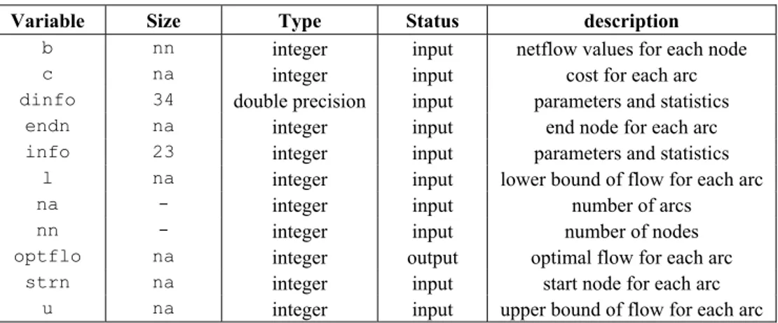
Table 2 – Arguments for pdnet().
Variable Size Type Status description
b nn integer input netflow values for each node
c na integer input cost for each arc
dinfo 34 double precision input parameters and statistics
endn na integer input end node for each arc
info 23 integer input parameters and statistics
l na integer input lower bound of flow for each arc
na - integer input number of arcs
nn - integer input number of nodes
optflo na integer output optimal flow for each arc
strn na integer input start node for each arc
u na integer input upper bound of flow for each arc
Table 3 – Network data structure.
Variable Dimension Type description
na - integer number of nodes
nn - integer number of arcs
strn na integer start node for each arc
endn na integer end node for each arc
b nn integer flow values for each node
c na integer cost for each arc
l na integer lower bound of flow for each arc
u na integer upper bound of flow for each arc
The reference implementations of the main program PDNET reads network data from an input file by invoking functions available in the Fortran module pdnet_read.f90. These functions build PDNET input data structures from data files in the DIMACS format [2] with instances of minimum cost flows problems. As illustrated in the PDNET module
fdriver.f90, we provide specialized interfaces used in Fortran programs using dynamic memory allocation.
4.3 Memory allocation
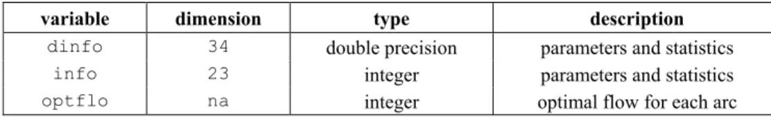
Table 4 – External arrays.
variable dimension type description
dinfo 34 double precision parameters and statistics
info 23 integer parameters and statistics
optflo na integer optimal flow for each arc
4.4 Parameter setting
PDNET execution is controlled by a variety of parameters, selecting features of the underlying algorithm and the interface with the calling program. A subset of these parameters is exposed to the calling procedure via a PDNET core subroutine. The remaining parameters are set at compile time with default values assigned in inside module
pdnet_default.f90.
The run time parameters listed in Tables 5 and 6 are set with Fortran function
pdnet_setintparm(). The integer parameters are assigned to components of vector
info and double precision parameters are assigned to vector dinfo.
4.5 Maximum flow computation
PDNET includes a maximum flow computation module called pdnet_maxflow, featuring the implementation of Goldfarb and Grigoriadis [6] of Dinic’s algorithm, that is used to check the maximum flow stopping criterion. Furthermore, a modification of this module, called pdnet_feasible, is called by the module pdnet_checkfeas() after reading the network file to compute a maximum flow on the network, therefore checking for infeasibility.
4.6 Running PDNET
Module fdriver inputs the network structure and passes control to module pdnet(). This subroutine starts by reading the control parameters from the vector info, with
pdnet_getinfo(). Correctness of the input is checked with pdnet_check(), and data structure created with pdnet_datastruct(). Internal parameters for methods are set with
pdnet_default(), and additional structures are created with pdnet_buildstruct(). Subroutines pdnet_transform() and pdnet_perturb() are called in order to shift the lower bounds to zero and to transform the data into double precision, respectively. Subroutines pdnet_probdata() and pdnet_checkfeas() check the problem characteristics and inquire if the network has enough capacity to transport the proposed amount of commodity. The primal-dual main loop is then started and the right-hand-side of the search direction system is computed by pdnet_comprhs(). The maximum spanning tree is computed by pdnet_heap(), and its optimality is tested by pdnet_optcheck(). Under certain conditions (µ<1), the maxflow stopping criterion is invoked by subroutine
We now present a usage example. Let us consider the problem of finding the minimum cost flow on the network represented in Figure 2. In this figure, the integers close to the nodes represent the node’s produced (positive value) or consumed (negative value) net flows, and the integers close to the arcs stand for their unit cost. Furthermore the capacity of each arc is bounded between 0 and 10. In Figure 3, we show the DIMACS format representation of this problem, stored in file test.min. Furthermore, Figures 4 and 5 show the beginning and the end of the printout given by PDNET, respectively.
Table 5 – List of runtime integer parameters assigned to vector info.
component variable description
1 bound used for building maximum spanning tree
2 iprcnd preconditioner used
3 iout output file unit (6: standard output)
4 maxit maximum number of primal-dual iterations
5 mxcgit maximum number of PCG iterations
6 mxfv vertices on optimal flow network
7 mxfe edges on optimal flow network
8 nbound used for computing additional data structures
9 nbuk number of buckets
10 pduit number of primal-dual iterations performed
11 root sets beginning of structure
12 opt flags optimal flow
13 pcgit number of PCG iterations performed
14 pf iteration level
15 ierror flags errors in input
16 cgstop flags how PCG stopped
17 mfstat maxflow status
18 ioflag controls the output level of the summary
19 prttyp printout level
20 optgap duality gap optimality indicator flag
21 optmf maximum flow optimality indicator flag
22 optst spanning tree optimality indicator flag
23 mr estimate of maximum number of iterations
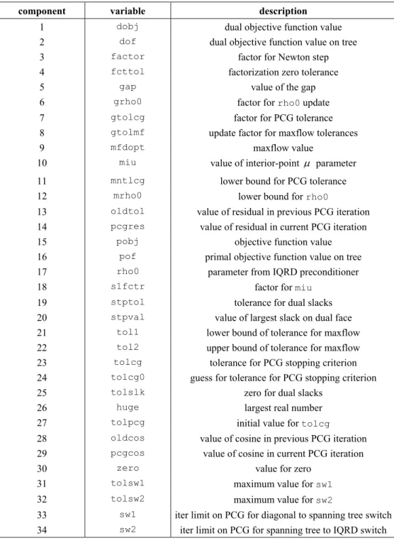
Table 6 – List of runtime double precision parameters assigned to vector dinfo.
component variable description
1 dobj dual objective function value
2 dof dual objective function value on tree
3 factor factor for Newton step
4 fcttol factorization zero tolerance
5 gap value of the gap
6 grho0 factor for rho0 update
7 gtolcg factor for PCG tolerance
8 gtolmf update factor for maxflow tolerances
9 mfdopt maxflow value
10 miu value of interior-point µ parameter
11 mntlcg lower bound for PCG tolerance
12 mrho0 lower bound for rho0
13 oldtol value of residual in previous PCG iteration
14 pcgres value of residual in current PCG iteration
15 pobj objective function value
16 pof primal objective function value on tree
17 rho0 parameter from IQRD preconditioner
18 s1fctr factor for miu
19 stptol tolerance for dual slacks
20 stpval value of largest slack on dual face
21 tol1 lower bound of tolerance for maxflow
22 tol2 upper bound of tolerance for maxflow
23 tolcg tolerance for PCG stopping criterion
24 tolcg0 guess for tolerance for PCG stopping criterion
25 tolslk zero for dual slacks
26 huge largest real number
27 tolpcg initial value for tolcg
28 oldcos value of cosine in previous PCG iteration
29 pcgcos value of cosine in current PCG iteration
30 zero value for zero
31 tolsw1 maximum value for sw1
32 tolsw2 maximum value for sw2
p min 4 5 n 1 2 n 2 -2 n 3 -4 n 4 4
a 1 2 0 10 3 a 2 4 0 10 -7 a 4 3 0 10 1 a 3 1 0 10 -4 a 2 3 0 10 2
Figure 3 – File test.min with the DIMACS format representation of the problem of Fig. 2.
Figure 4 – Startup and first two iterations of a typical PDNET session.
Figure 5 – Last iteration and results printout in typical PDNET session.
5. Computational results
A preliminary version of PDNET was tested extensively with results reported in [12]. In this section, we report on a limited experiment with the version of PDNET in the software distribution.
the instances of the test set netgen_lo were generated according to the guidelines stated in the computational study of Resende and Veiga [15], using the NETGEN generator following the specifications presented in Table 9. All these generators can be downloaded from the FTP site dimacs.rutgers.edu.
Table 7 – Specifications for instances in class mesh.
Problem n m maxcap maxcost seed x y xdeg ydeg
1 256 4096 16384 4096 270001 36 7 9 5
2 2048 32768 16384 4096 270001 146 14 9 5 3 8192 131072 16384 4096 270001 409 20 9 5
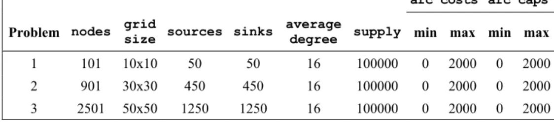
Table 8 – Specifications for instances in class grid.
arc costs arc caps
Problem nodes grid
size sources sinks
average
degree supply min max min max
1 101 10x10 50 50 16 100000 0 2000 0 2000 2 901 30x30 450 450 16 100000 0 2000 0 2000 3 2501 50x50 1250 1250 16 100000 0 2000 0 2000
Instances of increasing dimension were considered. The three netgen_lo instances presented were generated considering x=9, x=13 and x=15 respectively. In Table 10, the number of iterations (IT) and the CPU time (CPU) of PDNET and CPLEX 10 are compared. The reported results show that PDNET tends to outperform CPLEX in the larger instances of the mesh and netgen_lo set problems, but fails to do so in grid set problems. For testset netgen_lo the difference is quite noticeable for the largest instance. We observed that in this problem about 90% of the CPU time and iteration count in CPLEX 10 was spent computing a feasible solution. The results in this experience and those reported in [12] show that this code is quite competitive with CPLEX and other efficient network flow codes for large-scale problems.
6. Concluding remarks
Table 9 – NETGEN specification file for class netgen_lo.
seed Random number seed: 27001
problem Problem number (for output): 1
nodes Number of nodes: m=2x
sources Number of sources: 2
2x−
sinks Number of sinks: 2
2x−
density Number of (requested) arcs: 3
2x+
mincost Minimum arc cost: 0
maxcost Maximum arc cost: 4096
supply Total supply: 2( 2)
2 x−
tsources Transshipment sources: 0
tsinks Transshipment sinks: 0
hicost Skeleton arcs with max cost: 100%
capacitated Capacitated arcs: 100%
mincap Minimum arc capacity: 1
maxcap Maximum arc capacity: 16
Table 10 – Computational experience with instances of the sets mesh, grid and netgen_lo of test problems.
CPLEX 10 PDNET
Set Problem |V| |E| IT CPU IT CPU
1 256 4096 8383 0.04 40 0.08
mesh 2 2048 32768 108831 2.28 59 1.31
3 8192 131072 545515 51.06 76 10.20
1 101 1616 282 0.01 27 0.02
grid 2 901 14416 1460 0.03 35 0.36
3 2501 40016 4604 0.19 44 1.70
1 512 4102 3963 0.03 28 0.08
netgen_lo 2 8192 65709 135028 5.19 46 3.30
3 32768 262896 800699 112.24 59 27.50
References
(1) Ahuja, N.K.; Magnanti, T.L. & Orlin, J.B. (1993). Network Flows. Prentice Hall, Englewood Cliffs, NJ.
(2) DIMACS (1991). The first DIMACS international algorithm implementation challenge: Problem definitions and specifications. World-Wide Web document.
(4) El-Bakry, A.S.; Tapia, R.A. & Zhang, Y. (1994). A study on the use of indicators for identifying zero variables for interior-point methods. SIAM Review, 36, 45-72.
(5) Gay, D.M. (1989). Stopping tests that compute optimal solutions for interior-point linear programming algorithms. Technical report, AT&T Bell Laboratories, Murray Hill, NJ.
(6) Goldfarb, D. & Grigoriadis, M.D. (1988). A computational comparison of the Dinic and network simplex methods for maximum flow. Annals of Operations Research, 13, 83-123.
(7) International Organization for Standardization (1997). Information technology – Programming languages – Fortran – Part 1: Base language. ISO/IEC 1539-1:1997, International Organization for Standardization, Geneva, Switzerland.
(8) Karmarkar, N.K. & Ramakrishnan, K.G. (1991). Computational results of an interior point algorithm for large scale linear programming. Mathematical Programming, 52, 555-586.
(9) McShane, K.A. & Monma, C.L. & Shanno, D.F. (1989). An implementation of a primal-dual interior point method for linear programming. ORSA Journal on Computing, 1, 70-83.
(10) Mehrotra, S. & Ye, Y. (1993). Finding an interior point in the optimal face of linear programs. Mathematical Programming, 62, 497-516.
(11) Portugal, L.; Bastos, F.; Júdice, J.; Paixão, J. & Terlaky, T. (1996). An investigation of interior point algorithms for the linear transportation problem. SIAM J. Sci. Computing,
17, 1202-1223.
(12) Portugal, L.F.; Resende, M.G.C.; Veiga, G. & Júdice, J.J. (2000). A truncated primal-infeasible dual-feasible network interior point method. Networks, 35, 91-108.
(13) Prim, R.C. (1957). Shortest connection networks and some generalizations. Bell System Technical Journal, 36, 1389-1401.
(14) Resende, M.G.C. & Veiga, G. (1993). Computing the projection in an interior point algorithm: An experimental comparison. Investigación Operativa, 3, 81-92.
(15) Resende, M.G.C. & Veiga, G. (1993). An efficient implementation of a network interior point method. In: Network Flows and Matching: First DIMACS Implementation Challenge [edited by David S. Johnson and Catherine C. McGeoch], volume 12 of
DIMACS Series in Discrete Mathematics and Theoretical Computer Science, 299-348. American Mathematical Society.
(16) Resende, M.G.C. & Veiga, G. (1993). An implementation of the dual affine scaling algorithm for minimum cost flow on bipartite uncapacitated networks. SIAM Journal on Optimization, 3, 516-537.
(17) Ye, Y. (1992). On the finite convergence of interior-point algorithms for linear programming. Mathematical Programming, 57, 325-335.