http://dx.doi.org/10.1590/0103-6513.201415
1. Introduction
Operating cost forecasts together with revenues and capital expenditures compose the base for firms’ budgeting, which for many authors is the main tool of the management control system (Hansen et al., 2003; Lopes & Blaschek, 2007). Moreover, in period of crisis, especially, cost control is crucial. These authors also point out that the budgeting process still needs to be improved, which, among other claims, indicate a higher updating frequency. However, because this is an expensive process, the key consideration in defining the frequency of updates is the cost-benefit ratio.
Although the budget process is a widely studied theme in the international management accounting literature (Covaleski et al., 2006), Leite et al. (2008) found that in Brazil only 2.1% of master’s dissertations and 3.7% of doctoral thesis in the areas of business and accounting focused on budgeting. However, a later study by Moura et al. (2012) found a growing number of budgeting studies, although still 73% less than in the USA (Gomes et al., 2012).
Various articles (Vanzella & Lunkes, 2006; Bornia & Lunkes, 2007; Teixeira et al., 2011; Silva & Lavarda, 2014) have examined the subject more deeply and suggested improvements in the budget process, by incorporating additional methods like ABB (activity-based budgeting), Balanced Scorecard and TDABC (time-driven activity-based costing). Barbosa Filho
& Parisi (2006) and Frezatti (2005) discussed the Beyond Budgeting approach as an innovation when compared to traditional budget models. Merchant (2007) took a different approach and studied the effect of budget models and behavioral influences on management behavior and performance. In turn, Buzzi et al. (2014) included information asymmetry of managers as an element of budget slack. From a more behavioral perspective, Hainzemann & Lavarda (2011) carried out a theoretical study relating organizational culture and the budget planning and control process.
Among the available studies in the literature on budgeting, few have dealt with operating cost
Received: Mar. 11, 2015; Accepted: Jul. 18, 2016
Operating cost budgeting methods: quantitative
methods to improve the process
José Olegário Rodrigues da Silvaa, Graziela Fortunatob*, Sérgio Augusto Pereira Bastosa
aFucape Business School, Vitória, ES, Brazil
bPontifícia Universidade Católica do Rio de Janeiro, Rio de Janeiro, RJ, Brazil *[email protected]
Abstract
Operating cost forecasts are used in economic feasibility studies of projects and in budgeting process. Studies have pointed out that some companies are not satisfied with the budgeting process and chief executive officers want updates more frequently. In these cases, the main problem lies in the costs versus benefits. Companies seek simple and cheap forecasting methods without, at the same time, conceding in terms of quality of the resulting information. This study aims to compare operating cost forecasting models to identify the ones that are relatively easy to implement and turn out less deviation. For this purpose, we applied ARIMA (autoregressive integrated moving average) and distributed dynamic lag models to data from a Brazilian petroleum company. The results suggest that the models have potential application, and that multivariate models fitted better and showed itself a better way to forecast costs than univariate models.
Keywords
forecasts and methods of effectively calculating them. Park et al. (2003) defended that the existing estimating methods, such as regression model and artificial intelligence applications are improper and time-consuming to estimate costs in the construction industry. However, most of the papers refer to asymmetric information on budgetary slack, capital budgeting process, incentives, budget as a tool of managerial performance, budgetary participation and organizational effectiveness, and the role of budgetary information (Gomes et al., 2012; Silva & Lavarda, 2014). The focus of the budget in the view of many authors is in the organizational environment, such as the works of Brüggen & Luft (2011), Efferin
& Hopper (2007), Hartmann et al. (2010), and Marginson & Ogden (2005). Therefore, according to Silva & Lavarda (2014), researches that address the budget issue at the international level are long and run through several areas of knowledge such as economics, psychology, sociology, management, and accounting, but not econometrics.
For the petroleum sector and specifically with a probabilistic approach, we only identified the paper by Verre et al. (2009), whose method was Monte Carlo simulation to model uncertainties of ABC costing (activity-based costing). The results indicate advantages of the method, such as: reduced variation between the predicted and realized figures, from 15% to 3%; greater transparency of the process; increased quality of projections; and reduction of risks. Garcia et al. (2010) also used Monte Carlo simulation to forecast production costs. Their observations were focused on the privatization by the Brazilian government of the mining giant Companhia Vale do Rio Doce (CVRD, now called Vale), examining the expectation that the cost behavior would change under private control, an outcome that was supported by the results. Silva et al. (2007) questioned the traditional methods of predicting the cost behavior and suggested that econometric methods should be incorporated in the procedures. Thus, this study tries to fill this gap around budgeting processes.
Given the importance of the budget for organizations (Covaleski et al., 2006; Hansen et al., 2003; Lopes & Blaschek, 2007; Lunkes et al., 2011) and the relative lack of studies in this area (Gomes et al., 2012; Leite et al., 2008) and the relevance of accurate forecasting of operating costs, both for budget planning and economic valuation of projects (Verre et al., 2009), this article compares operational cost prediction methods for the budgeting process, identifying the ease of preparation and the impact on improving the quality of forecasts. These characteristics can help improve budget planning and economic feasibility
studies. The importance of this subject increases in crisis period when the costs are on focus.
For this purpose, we used the database of a Brazilian company in the upstream (exploration and production) oil and gas sector that employs ABC in its budgeting process. We applied univariate ARIMA models and dynamic multivariate models with lags to predict the budget data. The company in question prepares two annual budgets, to meet demands for planning and operational cost prediction for economic feasibility studies of various production projects.
In section 2 the theoretical framework is established, followed by section 3, which presents the methodology used in the work. In section 4 the results are analyzed, and finally in section 5, the final remarks are presented.
2. Theoretical framework
2.1. Importance of the budget to companies
The budget is the main tool of firms’ control system (Hansen & Mowen, 1996; Hansen et al., 2003; Hope
& Fraser, 2003; Lopes & Blaschek, 2007). According to Luft & Shields (2003) and Lunkes et al. (2011) the focus of most research in this area has been on themes such as the causes and effects on individual behavior, the causes and effects on the sub-units of organizations, the use of budget information in planning or control activities, the adoption of budgeting as an instrument to measure performance or determine rewards, and the role of organizational micro-processes.
reveal idle capacity, only paying attention to fixed and variable costs, and strictly financial focus in the reports prepared.
Neely et al. (2001) identify 12 weaknesses that are most often cited in the literature on budgetary control and analyze the advantages and disadvantages between improving the budget process or simply abandoning it. According to their findings, rolling forecast is the approach with the greatest potential for application. Among the weaknesses of budgets cited are that they are intensive in time and resources, they aggregate relatively little value, especially when considering the preparation time, and they are not updated often enough (usually only once a year).
In relation to innovation of the budgeting process and reduction of the problems generated by the traditional budget process, Frezatti (2005) examines the approach known as Beyond Budgeting. His article is a literature review on the theme and identifies studies focusing on innovations and the problems and characteristics of casting a new eye on budgeting. Barbosa Filho & Parisi (2006) particularly analyzed Beyond Budgeting in the Brazilian food company Sadia in 2003, finding that traditional budgeting should be abandoned to eliminate centralized management and corporate gamesmanship. This new budgeting model was found to be nearest the new management models adopted by the company. In the same line, Vanzella
& Lunkes (2006), in a study of an electric utility company, point to activity-based budgeting (ABS) as an element to improve the budgeting process. While in ABC, the aim is to obtain the cost per product, service or any other cost object starting from the use of resources and passing to the activities that consume them, in ABB, the budget of the activities is the starting point. Naturally, the former does not exist without the latter.
Lunkes (2007) contains an analysis of the evolution of the budget process. The author argues that although the entire control process has felt the effect of innovations, there are no new performance measures that add to its conception, leaving budgeting open to criticisms by executives and researchers. In addition to this, Hope & Fraser (2003) point out that the budget used to attain targets does not always follow the predefined strategy of the company. Therefore, Bornia & Lunkes (2007) suggest adding the entire Balanced Scorecard (BSC) concept to the budgeting process, i.e., alignment of the budget targets to the strategic indicators of the BSC.
According to Fisher et al. (2002), many firms use the budget, regardless of the budget type or costing method employed, as a mechanism to determine managers’ compensation, which can encourage underestimation of productive capacity, generating
budget slacks. These slack bias budgets and cause losses to companies, since they stimulate inefficiency. They are pitfalls whereby subordinates underestimate the production target to be able to surpass it and receive additional compensation for performance. Consequently, there is a reduction of remuneration of their superiors. These authors show that the use of the budget both as a basis for allocating scarce resources and for assessment of performance causes a significant increase in initial budget proposals, reduces budget slack and improves the performance of employees (subordinates).
Budget slack is thus critical for the use of the budget as an effective management instrument. This happens even when the budget is not used as a variable compensation instrument, because budget slack still results from the interest of managers to present better performance than forecast in the budget (Beuren & Wienhage, 2013).
2.2. Operating costs budgeting
Activity-based costing (ABC), a costing method broadly used, is based on the activities the firm performs in the various processes required to produce goods or render services, whether for end customers or for support purposes. It was developed by Kaplan
& Cooper (1998) in the 1980s and provides a way to better deal with indirect costs, by the analysis of activities, which are allocated to products by means of cost drivers (Horngren et al., 2000; Martins, 2003). ABC attributes costs to cost objects. First of all, resource consumption is traced to the respective activities and then from these to the cost objects. Hansen & Mowen (2001) stress that this tracing by drivers is at the center of the ABC approach. Further, according to Hansen & Mowen (2001), as well as Silva et al. (2007), cost objects can be products, customers, departments and processes, for which costs are measured and attributed. In turn, the activity is a basic unit of work performed within the organization. The drivers are the factors that cause changes in the consumption of resources, consumption of activities, costs and revenues.
The identification, analysis and allocation of costs to a firm’s processes aim to improve management of profitability. The use of this method allows better measurement of costs because it recognizes the causal relationships of the factors responsible for the costs of activities. This ameliorates the distortions caused by the use of apportionment in the traditional logic of cost absorption (Khoury & Ancelevicz, 2000).
because it is considered a longer run tool. According to Theeuwes & Adriaansen (1994) and Kee (2001), this limitation means ABC is not a suitable tool for making operational decisions. With the theory of constraints, Kee (2001) formulated a model called operational ABC that can be used in short-term operational decisions, the advantages of which were confirmed by Cogan (2005, 2006).
The information provided by the activity-based cost method can be used to improve the process of decision making, identifying opportunities to maximize profitability and efficiency, particularly if such a method is used in the company’s planning process, whose most obvious product is the corporate budget. Thus, the concept of activity-based budgeting (ABB) arises.
The operating cost in the petroleum industry, besides being considered in the budgeting of companies and economic analyses of new projects, also is important in certification of hydrocarbon (oil and gas) reserves, the main asset of firms in the industry. These reserves are periodically audited, and besides various technical criteria, they must be economically feasible, i.e., the operating cash flow must be positive until the end of the field’s lifetime. In Brazil, according to the National Petroleum, Natural Gas and Biofuels Agency (Agência Nacional do Petróleo, 2010, p. 8), “proven reserves are reserves of petroleum and natural gas that, based on the analysis of geological and engineering data, can be commercially recovered from reservoirs discovered”.
External factors, such as greater demand for services in the sector, reduced oil demand and wars can cause divergences in the estimates of oil companies. In this line, Schiozer et al. (2008) show there is a relation between the price of oil and operating costs, with severe implications for investment projects. Furthermore, another external factor that can cause changes in the behavior of production costs, observed by Garcia et al. (2010), is the privatization process
(based on the authors’ analysis of those effects on Companhia Vale do Rio Doce, now just called Vale).
According to Verre et al. (2009), forecasting operating costs, both in the initial development stages of fields and during the productive lifetime of mature fields, is one of the most critical steps in managing risk and uncertainties. This requires optimization of the extraction of hydrocarbons during the life cycle of the asset. The authors present the ABC method in an Italian oil company to estimate the development and operating costs with application of Monte Carlo simulation. According to them, the operating cost estimate was originally obtained by using a percentage of the capital expenditure or was based on historical data plus a contingency for the operational phase. They divided the costs into three categories: operating costs, costs of services, and administrative overhead. In turn, they separated the cost drivers into operation and maintenance, chemical products, well services, insurance, commissioning, logistics and direct personnel costs. The model was constructed and validated in different stages of a project for real cases. Initially, they performed a cost analysis, involving definition of all the activities, resources and estimates, and then performed a risk analysis considering the probabilities, and finally carried out benchmarking for comparison with existing projects in a particular area or country. The implementation of this method increased the precision of the operating cost budgeting by reducing the differences between the forecast and observed numbers.
2.3. Basic oil production scheme
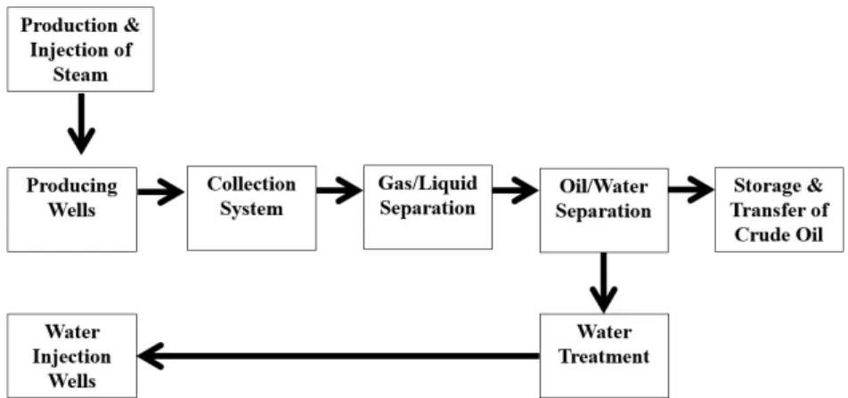
The content of this item was prepared based on Thomas (2004) and information obtained from technicians of the company studied. Figure 1 shows a simplified flowchart of the production and processing of crude oil, where production wells produce oil, gas
and water in varying proportions. Oil wells are equipped for production by natural lift (surge) or artificial lift. Natural lift (or elevation) generally occurs at the start of the field’s productive life, when the reservoir pressure is sufficient to push the fluid to the surface. Artificial elevation involves an additional energy source to lift the fluids to the surface. An example of artificial lift is the mechanical pump that is symbolic of the oil industry, known by various names (e.g., rocking horse, grasshopper, among many others). Gas wells normally produce non-associated gas (NAG), while water wells produce water for injection in other wells, aiming to repressurize the reservoir and consequently enhance the oil production.
The costs of operating wells, especially for intervention in production rigs to exchange lifting equipment, have large weight in the overall operating costs. The collection system consists of installations ranging from the producing wells to the primary processing station. Under the simplest arrangements, this basically consists of a complex system of pipes, manifolds (set of valves), tanks and pumps.
Gas-liquid separation is the first process that occurs at the treatment station or unit, where the gas is separated from the oil and water. This gas is compressed and undergoes a scrubbing process and is then transferred to a natural gas processing unit, after which it is ready to be distributed to the consumer market.
The oil-water separation, also known as oil treatment, is a step in which the oil-water emulsion is broken down by heating and applying chemical products called demulsifiers. The treated crude oil is then stored and transferred to a terminal or directly to refineries after measurement of the water content (which generally must be under 1%).
The water that is extracted along with the oil and gas (called produced water), after separation, requires treatment before being injected into the rock formation to increase the reservoir pressure and boost recovery, or being discharged into the ocean or an onshore water body. The treatment consists of removing oily and solid wastes by means of flotation and/or filtration.
Water injection wells receive the treated produced water. This is usually injected in the form of steam at high temperature and pressure, produced by steam generation units. This is particularly useful when the crude oil is heavy (highly viscous), by reducing the viscosity and increasing the flow. Depending on the producing field and processing methods, other processes can be present, such as gas injection (for supplementary recovery or storage) and CO2 injection.
3. Methodology
The objective of this article is to compare the forecasting methods for budgeting operating costs, to identify those that are easy to formulate and bring better predictions, following in the footsteps of Neely et al. (2001). According to those authors, companies want to find ways to make predictions more often and with the lowest possible cost, so as to maximize the cost-benefit ratio.
The data were provided by a Brazilian company involved in exploration and production with an onshore operation which uses ABC method, and consequently ABB. Besides the availability of the data, the lack of which is a common problem in similar studies (Leite et al., 2008; Lunkes et al., 2011), various other reasons contributed to the choice of the Brazilian petroleum sector: (i) the country’s market is relatively open, with the participation of national and foreign players; (ii) there are both large and small companies involved; (iii) the growth perspectives are strong, particularly from exploitation of the “pre-salt” reserves1; and (iv) petroleum has high importance in
the global economy.
In return for allowing us to use the data, the company required a confidentiality agreement, requiring no disclosure of its name or information that can identify the real cost amounts.
The data on operating costs and volume are monthly from January 2006 to December 2010. We multiplied the figures by a constant to comply with the confidentiality requirement. The operating cost spreadsheet contains approximately 22 thousand lines,
1 Some petroleum industry sources distinguish among
post-salt, pre-salt and subsalt reserves: “Post-salt
refers to crude oil and natural gas reservoirs lying above and deposited after an autochthonous (deposited in its present position) salt layer. Pre-salt refers to reservoirs lying beneath and deposited prior to an
autochthonous salt layer. Subsalt refers to reservoirs
lying beneath allochthonous (deposited at a distance from its present position) salt layers” (Chevron, 2013). Others use subsalt alone to describe the formations in Brazil: “Vast subsalt oil reserves have been uncovered in Brazil, the Gulf of Mexico and west Africa, but extreme pressure and inhospitable conditions have made extraction a challenge” (Lobo, 2012). Finally, some use subsalt and pre-salt as synonyms: “Brazil’s state-controlled oil producer Petrobras has reported a subsalt oil discovery in the fourth well drilled in the Jupiter area in the Santos Basin pre-salt block BM-S-24” (Offshore Technology.com, 2014). In deference to Brazilian
with information on costs in U.S. dollars segregated by: oil field, processing station, operational department, cost activities; and cost class. In turn, the physical data are volumes of fluids produced, injected or transported from operational wells, itemized monthly.
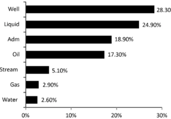
The company operates with 41 costs activities, classified into 7 cost objects, as shown in Figure 2: (1) Administration, (2) Water (treated and injected in wells), (3) Gas, (4) Liquid (oil + produced water), (5) Oil, (6) Wells and (7) Steam.
To exemplify, the cost objects received ABC values as follows: Oil received costs of activities directly related to the production and processing, such as storage, pumping and treatment. Administration refers to the common administrative costs that occur directly in the operational area. In Figure 2, it can be seen that the cost object Well has the greatest weight, accounting for 28.3% of the spending in the period analyzed, and that the four largest cost objects, Well (28.3%), Liquid (24.9%), Administration (18.9%) and Oil (17.3%) make up 89.4% of the total operating costs.
We chose these cost objects under the orientation of technicians of the company, since they represent the main intermediary products, with easily measured volumes. Thus, in this study, the budgeting process was based on such cost objects (Table 1), since it is a result of the demand for resources consumed in activities which are undertaken for the implementation of the cost object. To estimate costs based on cost objects implies considering efficiencies, strategic changes or even changes in the market or during the time. According to Ostrenga et al. (1997), the
activity-based costing is a technique to calculate costs of “objects.” Pamplona (1997) defended that the ABC technique can be easily understood in the cost object’s point of view: the objects are designed for activities that, in turn, consume resources, generating costs. Thus, the cost object accumulates the cost of all the activities involved in its production.
All the cost data in the period were corrected to real values with base date of January 2011 by the CPI (Consumer Price Index). The study period was 2006 to 2009, forming a set of 48 monthly cost and volume observations for each cost object. The year 2010 was the period for evaluation of the forecasts, when the projected data were compared against the observed figures.
The unit costs for each object were calculated monthly, by dividing the total cost by the respective physical value (volume), as shown in Equation 1.
Cunn,i = CTn.i / Qn,I (1)
Where: n is the cost object (varies from 1 to 7); i is the period analyzed; Cunn,i is the unit cost of object n referring to period i; CTn.i is the total cost of object n referring to period i; and Qn,i is the physical figure (flow or number of wells) of object n referring to period i.
To start the cost prediction, we employed univariate models that only consider the variable of interest, in which the forecast is based on its past values. Here, we analyze time series which it is supposed to be stationarity to be estimated by regression analysis. A stationary time series is supposed to present constant mean and variance over time and the value of the covariance between two periods only depend on the gap between these two periods. The stationarity can also be evaluated by the series unit root (Wooldridge, 2006). Therefore, if a time series is stationary, it can be analyzed by several ways.
Firstly, we adopted the ARMA (p,q) univariate model, according to Equation 2:
Yt = α + ϕ1Yt-1 + ϕ2Yt-2 + ... + ϕpYt-p +
εt + θ1εt-1 + θ2εt-2 +... θqεt-q+ ut (2)
Where: α denotes a constant; Yt-i represents the variables at t and lagged at i; ϕ1 and θ1 are the coefficients of the autoregressive terms and moving
Table 1. Basic differences of the budget process between the company and this study.
COMPANY THIS STUDY
Projects the unit cost per activity - 41 units. Projects the unit cost per cost object - 7 units.
The unit cost is fixed and calculated with the average of the past 12 months.
The unit cost varies with the physical quantities of each cost object and is defined based on regression of all historical data.
Source: Elaborated by the authors.
averages, in this order; εt represents the white noise at t and lagged at q and ut represents the error at t.
To verify the stationarity of the series, we apply the Dickey-Fuller (ADF) and Phillips-Perron (PP) tests, which consider the existence of a unit root in the null hypothesis. If the series is not stationary, i.e., presents a unit root, it is necessary to distinguish it, resulting in the ARIMA (p,d,q) model. If the series presents a seasonal component, it must be represented by the SARIMA (p,d,q) model.
In general, modeling of time series involves four steps (Wooldridge, 2006): identification of the process MA(q) and AR(q) for stationary series and a step further with the “d” order for a non-stationary series; estimation of the model by OLS (Ordinary Least Squares); diagnostic tests by AIC (Akaike’s Information Criteria) and BIC (Bayesian Information Criteria) – choose the ones which present the lowest error; and extracting the predictions of the model based on the RMSE (root mean square error), MPE (mean percentage error), and MAPE (mean absolute percentage error). We carried out all those steps, but to save space they are only partially presented.
Next we employed dynamic distributed lag models, which are the most general form of dynamic models. They work with the dependent variable Y and the independent variables X, and lagged values of Y and X, according to Equation 3:
Yt = α + ϕ1Yt-1 + ϕ2Yt-2 + ... + ϕpYt-p +
θ1Xt-1 + θ2Xt-2 +... θqXt-q+ εt (3)
In this equation, p and q represent the orders of the lags; and α, ϕ and θ are the coefficients.
According to Hansen & Mowen (2001), forecasting the cost component can be done using linear regression, which in turn can have one or more explanatory variables. If there are more than one variable, then it is a case of multiple linear regression.
The models analyzed in this study follow the concept currently used by the company, but with the
insertion of procedures, such as regression, aiming to improve the forecasting quality. The basic differences between the procedures followed by the company in its budgeting process and those analyzed here are shown in Table 1.
The general formula to calculate the total operating cost forecast for each period is presented in Equation 4. In it, the unit costs of the various cost objects are multiplied by the respective physical quantities in the period, composing the total cost.
CTi = ∑ Cunn,,i x Qn,,I (4)
In this equation, n is the cost object; i is the period analyzed; Cunn,i is the unit cost of object n referring to period i; Qn,i is the physical figure of object n referring to period I; and CTi is the total cost in period i.
In the next section the results are analyzed.
4. Analysis of the results
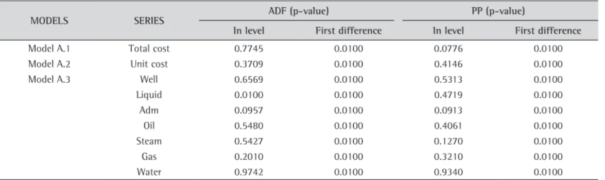
To check for the existence of a unit root, and hence stationarity of the series, we applied the augmented Dickey-Fuller (ADF) and Phillips-Perron (PP) tests, which have a null hypothesis of the existence of a unit root, as described before. The results are presented in Table 2, where it can be seen that except for the Liquid series, all the others have a unit root, verified by the ADF and PP tests. However, in first difference, all the series are stationary according to both tests.
Hence, the series being nonstationary, it means that they follow the ARIMA (p.d,q) process.
4.1. Univariate model: ARIMA – Models A
The models used in this analysis of nonstationary series are autoregressive integrated moving average (ARIMA) models. To identify the most efficient models for prediction, we analyzed the following ones:
Table 2. Unit root test statistics: Model A.
MODELS SERIES ADF (p-value) PP (p-value)
In level First difference In level First difference
Model A.1 Total cost 0.7745 0.0100 0.0776 0.0100
Model A.2 Unit cost 0.3709 0.0100 0.4146 0.0100
Model A.3 Well 0.6569 0.0100 0.5313 0.0100
Liquid 0.0100 0.0100 0.4719 0.0100
Adm 0.0957 0.0100 0.0913 0.0100
Oil 0.5480 0.0100 0.4061 0.0100
Steam 0.5427 0.0100 0.1270 0.0100
Gas 0.2010 0.0100 0.3210 0.0100
Water 0.9742 0.0100 0.9340 0.0100
Note: 5% significance level.
Model A.1→ ARIMA (p,d,q) model, suitable to forecast the total cost series;
Model A.2→ ARIMA (p,d,q) model, suitable to forecast unit cost series (cost per volume of oil equivalent). In this case, to obtain the total cost it is necessary to multiply the unit cost by the production of oil equivalent (oil + gas);
Model A.3→ ARIMA (p,d,q) model, for the unit cost of each of the cost objects identified. The total cost is the sum of the unit costs of the objects multiplied by the corresponding physical figure (flow or number of wells).
4.1.1. Estimation of Models A
After checking for unit roots, we then estimated the models themselves: Model A.1, forecast of total cost; Model A.2, forecast of unit cost of oil equivalent (volume of oil and gas); and Model A.3, forecast of unit cost for each cost object.
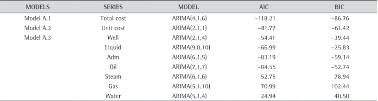
For each series we estimated between 500 and 1,000 univariate models of the ARIMA (p,d,q) type, and chose the ones with the lowest values of the Akaike information criterion (AIC) and Bayesian information criterion (BIC), lowest error and with autocorrelation within the significance range of 5%. The models indicated and their respective information criteria values are shown in Table 3.
The proposed models were validated by verifying the residuals (white noise) by means of autocorrelation and heteroscedasticity tests. For autocorrelation we used the Ljung-Box test, whose null hypothesis is the absence of serial autocorrelation, while for heteroscedasticity we used the Breusch-Pagan-Godfrey
test, whose null hypothesis is that the data series is homoscedastic. At 5% significance, the tests indicated the absence of homoscedasticity and serial autocorrelation (Appendix A).
4.1.2. Forecast of Models A
The final step of the modeling – prediction of the models – was carried out by measuring the performance or forecasting quality indicators, based on the RMSE (root mean square error), MPE (mean percentage error) and MAPE (mean absolute percentage error). Table 4 presents the forecasting errors of the models in the period from 2006 to 2009, so that the last (2010) could serve as a base for comparison. Considering the analyses for prediction, models A.1 and A.2 presented good results, especially when considering the MPE as reference.
Model A.1, based on the total cost, has a more stable profile than model A.2, whose prediction was based on the unit cost of oil equivalent. This is due to the fact that the final cost of model A.2 is impacted by the physical quantities of the drivers.
4.2. Dynamic distributed lag models:
Models B
Next we estimated new models, now multivariate, by means of multiple regression, including endogenous and exogenous variables, autoregression and lags. However, here we only present the results of the models that performed the best, both from the standpoint of errors and of the diagnostic tests.
Table 3. Univariate ARIMA Model: Model A.
MODELS SERIES MODEL AIC BIC
Model A.1 Total cost ARIMA(4,1,6) –118.21 –86.76
Model A.2 Unit cost ARIMA(2,1,1) –81.77 –61.42
Model A.3 Well ARIMA(2,1,4) –54.41 –39.44
Liquid ARIMA(9,0,10) –66.99 –25.83
Adm ARIMA(6,1,5) –83.19 –59.14
Oil ARIMA(7,1,7) –84.55 –52.74
Steam ARIMA(6,1,6) 52.75 78.94
Gas ARIMA(5,1,10) 70.99 102.44
Water ARIMA(5,1,4) 24.94 40.50
Note: 5% significance level.
Source: Elaborated by the authors with Eviews 6.0.
Table 4. Forecasting performance from 2006 to 2009: Model A.
MODEL RMSE MPE MAPE
Model A.1 79.4 1.34% 4.54%
Model A.2 98.3 1.60% 5.48%
Model A.3 103.8 3.76% 5.53%
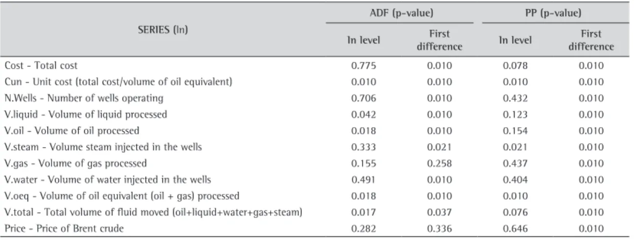
Table 5 presents the unit-root test statistics for the series utilized to formulate the dynamic model with the ADF and PP tests.
The series were calculated by taking the natural logarithm of the data. According to the results presented in Table 5, the series Cun, V.liquid, V.oil, V.oeq and V.total do not have a unit root in level and are considered stationary. At 10% significance, the Cost series also can be considered stationary by the PP test, as can the series Cun, V.steam, V.oeq and V.total.
4.2.1. Estimation of the Models B
In this step, we constructed the models to check the relationship between costs (Total cost and Unit cost) and the physical data and lags, both for the costs and other variables.
Of the models estimated, those with highest adjusted R2 are listed in Table 6. All the models
presented statistical significance and Models B.2, B.6 and B.8 presented coefficients of determination greater than 0.9.
We should stress that the possibility of working with series in level satisfies the premise of identifying models that are easy to execute and manipulate by technical staff who do not have specific knowledge of forecasting tools.
To validate the proposed models, we analyzed the residuals be means of tests of autocorrelation, heteroscedasticity and normality. For autocorrelation we again used the Ljung-Box test, whose null hypothesis is the absence of serial autocorrelation. For heteroscedasticity we used the Breusch-Pagan-Godfrey test, where the null hypothesis is that the series is homoscedastic. Finally, for normality we applied the Jarque-Bera test, whose null hypothesis is that the data are normally distributed (Appendix A).
At 5% significance, the results indicate the absence of serial autocorrelation (except for models B.5 and B.6), that the series are homoscedastic and the residuals are normally distributed (except for model B.5). Therefore, there is evidence that the estimated models (except for B.5 and B.6) present white noise and capture the necessary information to provide a good result to forecast operating costs.
Table 5. Unit-root test statistics: Model B.
SERIES (ln)
ADF (p-value) PP (p-value)
In level First
difference In level
First difference
Cost - Total cost 0.775 0.010 0.078 0.010
Cun - Unit cost (total cost/volume of oil equivalent) 0.010 0.010 0.010 0.010
N.Wells - Number of wells operating 0.706 0.010 0.432 0.010
V.liquid - Volume of liquid processed 0.042 0.010 0.123 0.010
V.oil - Volume of oil processed 0.018 0.010 0.154 0.010
V.steam - Volume steam injected in the wells 0.333 0.021 0.021 0.010
V.gas - Volume of gas processed 0.155 0.258 0.437 0.010
V.water - Volume of water injected in the wells 0.491 0.010 0.404 0.010
V.oeq - Volume of oil equivalent (oil + gas) processed 0.018 0.010 0.010 0.010
V.total - Total volume of fluid moved (oil+liquid+water+gas+steam) 0.017 0.037 0.076 0.010
Price - Price of Brent crude 0.282 0.336 0.646 0.010
Note: 10% significance.
Source: Elaborated by the authors with Eviews 6.0.
Table 6. Models with lags: Model B.
MODELS Adjusted R2 F (p-value)
Model B.1 Cost = f(N.wells, V.liquid, V.oil, V.steam, V.gas, V.water) 0.6328 1.23E-07
Model B.2 Cun = f(N.wells, V.liquid, V.oil, V.steam, V.gas, V.water) 0.9104 6.70E-20
Model B.3 Cost = f(Cun(-1), Cun(-2), Cun(-3), Cun(-4), V.total) 0.6932 1.48E-10
Model B.4 Cun= f(Cun(-1), Cun(-2), Cun(-3), Cun(-4), V.total) 0.8392 1.65E-16
Model B.5 Cost = f(Cost(-1), Cost (-2), Cost(-3), Cost(-4), V.oeq, Price) 0.7652 3.28E-12
Model B.6 Cun = f(Cun(-1), Cun(-2), Cun(-3), Cun(-4), V.oeq, Price) 0.9524 2.43E-22
Model B.7 Cost = f(Cost(-1), Cost(-2), Cost(-3), Cost(-4), V.oeq, V.oeq(-1)) 0.7822 4.46E-10
Model B.8 Cun = f(Cun(-1), Cun(-2), Cun(-3), Cun(-4), V.oeq, V.oeq(-1)) 0.9463 1.58E-25
Note: 5% significance level.
4.2.2. Forecasts of Models B
Table 7 presents the RMSE (root mean square error), MPE (mean percentage error) and MAPE (mean absolute percentage error). The models were estimated in the period from 2006 to 2009 and 2010 served as the base for comparison.
From Table 7, it can be seen that model B.5 presented the smallest prediction errors (69.5, –1.07% and 3.32%). However, this model had problems in the diagnostic tests and there is evidence that its residuals are not characterized as white noise.
Among the other models, the most suitable is B.8, with the lowest forecasting errors (74.5, –1.86% and 3.52%) and the second highest coefficient of determination (adjusted R2 = 0.9463). Model B.6 also
showed small prediction errors (72.1, 1.49% and 3.89%), but it also presented evidence of heteroscedasticity. Based on these results, we applied regression to analyze model B.8. The results are shown in Table 8, where it can be seen that all the regression coefficients are significant at 5%, indicating this is a good forecasting model.
5. Final remarks
This study investigated methods to forecast operating costs using univariate ARIMA models and multivariate models with distributed lags. The models were tested with data between January 2006 and December 2010 from a Brazilian petroleum company with upstream (exploration and production) activities.
Specifically, we used data from 2006 through 2009 as the base to analyze the models, forming a set of 48 monthly observations of costs and volumes per cost object, and then used the data from 2010 to evaluate the forecasts, by comparing the projected data against the observed numbers.
More specifically, we developed two groups of models: (A) univariate ARIMA models, whose analysis was based on total operating cost and unit cost of oil equivalent (oil and gas); and (B) multivariate dynamic models with distributed lags, analyzed based on total operating cost or unit cost of oil in function of the respective lags and the physical data of the cost objects.
We analyzed the models’ performance by means of the forecasting quality indicators RMSE (root mean square error), MPE (mean percentage error) and MAPE (mean absolute percentage error). The results demonstrated that the estimated models, both univariate and multivariate, have potential business application, since the MAPE values were between 3.5% and 6.0% in the majority of the results.
Since the company adopts an annual base for consolidation and follow-up of the budget, the MPE appears to be the best measure for comparison between the predicted and observed numbers. By this metric, five models had MPE values below 2.0% (two ARIMA models and three dynamic multivariate models).
Assuming the errors (MAPE and MPE) as the main criteria for choice, the results indicate that model B.8 is the most suitable for predicting the operating cost based on the sample studied. In that model, the
Table 7. Forecasting performance from 2006 to 2009: Model B.
MODEL RMSE MPE MAPE
Model B.1 189.3 –6.85% 8.12%
Model B.2 180 –7.31% 8.01%
Model B.3 86.5 –4.67% 4.37%
Model B.4 127 –3.52% 7.11%
Model B.5 69.5 –1.07% 3.32%
Model B.6 72.1 1.49% 3.89%
Model B.7 105.7 –4.66% 5.05%
Model B.8 74.5 –1.86% 3.52%
Source: Elaborated by the authors with Eviews 6.0.
Table 8. Regression statistics of Model B.8.
Variable Coefficients t-statistic p-value Statistics
Intersection 2.7609 3.4496 0.0013 R multiple: 0.9728
Cun(-1) 0.6064 5.9395 0.0000 R-squared: 0.9463
Cun(-3) –0.2593 –3.0658 0.0038 Adjusted R squared: 0.9399
Cun(-4) 0.3458 4.7198 0.0000 Standard error: 0.0552
V.oeq –1.1847 –9.9649 0.0000 Observations: 48
V.oeq(-1) 0.6743 3.9321 0.0003 p-value (F for significance): 1.58E-25
Note: 5% significance level.
forecast is the unit cost of oil with autoregressive terms and with the volume of oil equivalent (oil + gas) variable having lags.
According to the final results, the procedures tested, mainly multivariate dynamic models with distributed lags, can be carried out quickly, in line with the indications of Neely et al. (2001), who concluded that companies would like more frequent forecasts with a favorable cost-benefit ratio.
This study contributes to the process of preparing budgets, indicating that quantitative estimation methods can be of great value, both in terms of objectivity/simplicity of use and in terms of precision of the projections, notably regarding operating costs resulting from mature activities.
As proposals for future studies, we can suggest: (i) analyzing the behavior of models over a longer period and checking the contribution to certification of hydrocarbon reserves; and (ii) developing models for segregation of operating cost into its fixed and variable components and examining the behavior of fixed costs over the medium and long run.
References
Agência Nacional do Petróleo. (2010). Regulamento técnico Nº 001/2000 de reservas de petróleo e Gas natural: portaria nº 009. Brasília: ANP. Retrieved in 11 March 2015, from http://www.engelog.com/siteengelog/press/ press_information_files/press_brazil_information _files/ legislation_mid_fset_files/prod-transp_mid_fset_files/ prod-transp_text_files/anp _9_00.pdf
Barbosa Filho, F., & Parisi, C. (2006). Análise da aderência ao modelo beyond budgeting round table: o caso Sadia SA. Revista Universo Contábil, 2(1), 26-42. Retrieved in 11 March 2015, from http://www.spell.org.br/documentos/ download/26269
Beuren, I. M., & Wienhage, P. (2013). Folga organizacional no processo de gestão do orçamento: um estudo de caso no SENAC de Santa Catarina. REAd: Revista Eletrônica de Administration, 75(2), 274-300. http://dx.doi.org/10.1590/ S1413-23112013000200001.
Bornia, A. C., & Lunkes, R. J. (2007). Uma contribuição à melhoria do processo orçamentário. Contabilidade Vista & Revista, 18(4), 37-59. Retrieved in 11 March 2015, from http://www.spell.org.br/documentos/ver/25344/uma-contribuicao-a-melhoria-do-processo-orcamentario/i/pt-br Brimson, J. A., & Antos, J. (1999). Driving value using
activity-based budgeting. New York: John Wiley & Sons. Brüggen, A., & Luft, J. (2011). Capital rationing, competition,
and misrepresentation in budget forecasts. Accounting, Organizations and Society, 36(7), 399-411. http://dx.doi. org/10.1016/j.aos.2011.05.002.
Buzzi, D. M., Dos Santos, V., Beuren, I. M., & Faveri, D. B. (2014). Relação da folga orçamentária com participação e ênfase no orçamento e assimetria da informação. Revista Universo Contábil, 10(1), 6-27. http://dx.doi.org 10.4270/ RUC.2014101.
Chevron. (2013). Chevron glossary of energy and financial terms. San Ramon: Chevron. Retrieved in 02 September
2013, from https://www.chevron.com/-/media/chevron/ shared/documents/GlossaryOfEnergyAndFinancialTerms.pdf Cogan, S. (2005). Teoria das restrições versus outros métodos
de custeio: uma questão de curto prazo ou de longo prazo. Revista Universo Contábil, 1(3), 8-20.
Cogan, S. (2006). Modelo de Custeio Baseado em Atividades Aplicado a Decisões de Produção de Curto Prazo. Contabilidade Vista & Revista, 17(1), 11-27. Retrieved in 11 March 2015, from http://www.redalyc.org/articulo.oa?id=197014749002 Covaleski, M. A., Evans Iii, J. H., Luft, J. L., & Shields, M. D.
(2006). Budgeting research: three theoretical perspectives and criteria for selective integration. Handbook of Management Accounting Research, 2, 587-624. http:// dx.doi.org/10.1016/S1751-3243(06)02006-2.
Efferin, S. A., & Hopper, T. (2007). Management control, culture and ethnicity in a Chinese Indonesian company. Accounting, Organizations and Society, 32(3), 223-262. http://dx.doi.org/10.1016/j.aos.2006.03.009.
Fisher, J., Maines, L. A., Peffer, S. A., & Sprinkle, G. B. (2002). Using budgets for performance evaluation: effects of resource allocation and horizontal information asymmetry on budget proposals, budget slack, and performance. Accounting Review, 77(4), 847-865. http://dx.doi. org/10.2308/accr.2002.77.4.847.
Frezatti, F. (2005). Beyond budgeting: inovação ou resgate de antigos conceitos do orçamento empresarial? Revista de Administration Eletrônica: RAE, 45(2), 23-33.
Garcia, S., Lustosa, P. R. B., & Barros, N. R. (2010). Aplicabilidade de métodos de simulação de Monte Carlo na previsão de custos de produção de companhia industriais: o caso da companhia Vale do Rio Doce. Revista de Contabilidade e Organizações, 4(10), 152-173. http://dx.doi.org/10.11606/ rco.v4i10.34781.
Gomes, G., Lavarda, C. E. F., & Torrens, E. W. (2012). Revisão da literatura sobre orçamento em cinco periódicos internacionais nos anos de 2000 até 2009. REGE Revista de Gestão, 19(1), 107-123.
Hainzemann, L. M., & Lavarda, C. E. F. (2011). Cultura organizacional e o processo de planejamento e controle orçamentário. Revista de Contabilidade e Organizações, 5(13), 4-19. http://dx.doi.org/10.11606/rco.v5i13.34801. Hansen, D. R., & Mowen, M. M. (1996). Cost management:
accounting and control. Cincinnati: South Western. Hansen, D. R., & Mowen, M. M. (2001). Gestão de custos:
contabilidade e controle. São Paulo: Pioneira Thomson Learning.
Hansen, S. C., Otley, D. T., & Van Der Stede, W. A. (2003). Practice developments in budgeting: an overview and research perspective. Journal of Management Accounting Research, 15(1), 95-116. http://dx.doi.org/10.2308/ jmar.2003.15.1.95.
Hartmann, F., Naranjo-Gil, D., & Perego, P. (2010). The effects of leadership styles and use of performance measures on managerial work-related attitudes. European Accounting Review, 2(19), 275-310. http://dx.doi. org/10.1080/09638180903384601.
Hope, J., & Fraser, R. (2003). Beyond budgeting: how managers can break free from the annual performance trap. Boston: Harvard Business School Press.
Offshore Technology.com. (2014). Kongsberg to support Statoil’s Johan Castberg project. London. Retrieved in 14 August 2014, from http://www.offshore-technology.com/news/ company-news/20
Ostrenga, M. R., Ozan, T. R., McIlhattan, R. D., & Harwood, M. D. (1997). Guia da Ernst & Young para gestão total dos custos. Rio de Janeiro: Record.
Pamplona, E. D. O. (1997). Contribuição para a análise crítica do sistema de custos ABC através da avaliação de direcionadores de custos (Tese de Doutorado). Escola de Administração de Empresas de São Paulo, Fundação Getúlio Vargas, São Paulo.
Park, C., Hong, S., Kim, C., & Lee, J. (2003). A budget estimating method of environmental cost for multiple housing projects. In Proceedings of the AACE International Transactions, ES241, Orlando, Florida.
Schiozer, R. F., Lima, G. A., & Suslicks, S. B. (2008). The pitfalls of capital budgeting when costs correlate to oil price. Journal of Canadian Petroleum Technology, 47(8), 12-14. http://dx.doi.org/10.2118/08-08-57.
Silva, F. D. C., Vasconcelos, M. T. C., Silva, A. C. B., & Campelo, S. M. (2007). Comportamento dos custos: uma investigação empírica acerca dos conceitos econométricos sobre a teoria tradicional da contabilidade de custos. Revista Contabilidade e Finanças, 43, 61-72. Retrieved in 11 March 2015, from http://www.scielo.br/pdf/rcf/v18n43/a06v1843.pdf Silva, M. Z., & Lavarda, C. E. (2014). Orçamento empresarial:
estudo comparativo entre publicações nacionais e internacionais. BASE: Revista de Administração, 11(3), 179-192. Retrieved in 11 March 2015, from http://www. redalyc.org/articulo.oa?id=337232427002
Teixeira, A. J. C., Gonzaga, R. P., Santos, A. V. S. M., & Nossa, V. (2011). A utilização de ferramentas de contabilidade gerencial nas empresas do Estado do Espírito Santo. BBR: Brazilian Business Review (Federal Reserve Bank of Philadelphia), 8(3), 108-127.
Theeuwes, J. A. M., & Adriaansen, J. K. M. (1994). Towards an integrated accounting frameworks for manufactoring improvement. International Journal of Production Economics, 36(1), 85-96. http://dx.doi.org/10.1016/0925-5273(94)90151-1.
Thomas, J. E. (2004). Fundamentos da Engenharia de Petróleo. Rio de Janeiro: Interciência.
Vanzella, C., & Lunkes, R. J. (2006). Orçamento baseado em atividades: um estudo de caso em empresa distribuidora de energia elétrica. Contabilidade Vista & Revista, 17(1), 113-132.
Verre, F., Giubileo, A., & Cadegiani, C. (2009). Asset life-cycle OPEX modelling with Monte Carlo simulation to reduce uncertainties and to improve field exploitation. In Proceedings of the SPE Annual Technical Conference and Exhibition, New Orleans, USA. http://dx.doi.org/10.2118/124230-MS. Wooldridge, J. M. (2006). Introdução à Econometria. São Paulo:
Thomson Learning. Kaplan, R. S., & Cooper, R. (1998). Cost & effect: using integrated
cost systems to drive profitability and performance. Brighton: Harvard Business Press.
Kee, R. C. (2001). Evaluating the economics of short- and long-run production: related decisions. Journal of Managerial Issues, 13(2), 139-158.
Khoury, C. Y., & Ancelevicz, J. (2000). Controvérsias acerca dos sistemas de custos ABC. Revista de Administração de Empresas, 40(1), 56-62. http://dx.doi.org/10.1590/ S0034-75902000000100007.
Leahy, T. (2002). As 10 maiores armadilhas do orçamento. HSM Management, 32, 1-5.
Leite, R. M., Silva, H. F. N., Cherobim, A. P. M. S., & Bufrem, L. S. (2008). Orçamento Empresarial: levantamento da produção científica no período de 1995 a 2006. Revista Contabilidade e Finanças, 19(47), 56-72. http://dx.doi. org/10.1590/S1519-70772008000200006.
Lobo, R. (2012). Big oil sinks to the depths. The New Economy. Retrieved in 03 October 2012, from http://www. theneweconomy.com/energy/big-oil-sinks-to-the-depths Lopes, H. A., & Blaschek, J. R. S. (2007). Minimizando as
deficiências do planejamento operacional com o uso do orçamento baseado em atividades. Revista de Contabilidade do Mestrado em Ciências Contábeisda Uerj, 12(2), 1-16. Luft, J., & Shields, M. D. (2003). Mapping Management
accounting: graphics and guidelines for theory consistent empirical research. Accounting, Organizations and Society, 28(2), 169-249. http://dx.doi.org/10.1016/S0361-3682(02)00026-0.
Lunkes, R. J. (2007). Manual de orçamentos. São Paulo: Atlas. Lunkes, R. J., Feliu, V. M. R., & Rosa, F. S. (2011). Pesquisa
sobre o orçamento na Espanha: um estudo bibliometrico das publicações em contabilidade. Revista Universo Contábil, 7(3), 112-132. http://dx.doi.org/10.4270/ruc.2011325. Marginson, D., & Ogden, S. (2005). Coping with ambiguity
through the budget: the positive effects of budgetary targets on managers’ budgeting behaviors. Accounting, Organizations and Society, 30(5), 435-456. http://dx.doi. org/10.1016/j.aos.2004.05.004.
Martins, E. (2003). Contabilidade de custos. São Paulo: Atlas. Merchant, K. A. (2007). Modelo do Sistema de orçamento
corporativo: influências no comportamento e no desempenho gerencial. Revista de Contabilidade e Organizações, 1(1), 104-121. http://dx.doi.org/10.11606/rco.v1i1.34700. Moura, G. D., Dallabona, L. F., & Lavarda, C. E. F. (2012).
Perfil dos estudos sobre o tema orçamento publicados em congressos brasileiros, de 2005 a 2009. Revista Contabilidade Vista & Revista, 23(1), 97-125. Retrieved in 11 March 2015, from http://www.redalyc.org/articulo. oa?id=197026232006
Appendix A. Ljung-box and Breusch-Pagan-Godfrey and Jarque-Bera Tests.
Models A. Ljung-box and breusch-pagan-godfrey tests.
MODELS
p-value
Autocorrelation Heteroscedasticity Ljung-Box test Breush-Pagan Godfrey
Model A.1 Total cost 0.9992 0.0791
Model A.2 Unit cost 0.9640 0.1692
Model A.3
Well 0.9646 0.3146
Liquid 0.9322 0.2839
Adm 0.7711 0.2848
Oil 1.0000 0.1973
Steam 0.9984 0.7145
Gas 0.9996 0.3148
Water 0.9537 0.2840
Note: 5% significance level.
Source: Elaborated by the authors with Eviews 6.0.
Models B. Ljung-box and breusch-pagan-godfrey and jarque-bera tests.
MODELS
p-value
Autocorrelation Heteroscedasticity Normality Ljung-Box test Breush-Pagan Godfrey Jarque-Bera
Model B.1 0.6312 0.2247 0.3188
Model B.2 0.3205 0.5845 0.3293
Model B.3 0.4646 0.1641 0.6019
Model B.4 0.1094 0.1837 0.7851
Model B.5 0.0451 0.1375 0.0494
Model B.6 0.0355 0.3710 0.7333
Model B.7 0.5026 0.1747 0.9546
Model B.8 0.2424 0.4801 0.1479
Note: 5% significance level.