USE DATA FROM PERMANENT SAMPLING POINTS IN GROWTH AND
YIELD MODELING¹
Alexandre José Pereira2, Helio Garcia Leite3, João Carlos Chagas Campos3 e Agostinho Lopes de Souza3
ABSTRACT: This study was carried to evaluate the efficiency of the Bitterlich method in growth and yield modeling of the even-aged Eucalyptus stands. 25 plots were setup in Eucalyptus grandis cropped under a high bole system in the Central Western Region of Minas Gerais, Brazil. The sampling points were setup in the center of each plot. The data of four annual mesurements were colleted and used to adjust the three model types using the age, the site index and the basal area as independent variables. The growths models were fitted for volume and mass of trees. The efficiency of the Bitterlich method was confirmed for generating the data for growth and yield modeling.
Keywords: Growth and yield models, permanent sampling points, Bitterlich method.
USO DE DADOS DE PARCELAS PERMANENTES DE ÁREA VARIÁVEL EM
MODELAGEM DE CRESCIMENTO E DA PRODUÇÃO
RESUMO: Este estudo foi conduzido visando avaliar a eficiência do método de Bitterlich para gerar dados para estudos de crescimento e produção. 25 parcelas de área fixa foram instaladas em um povoamento de
Eucalyptus grandis sob regime de alto fuste, localizado na região centro-oeste do Estado de Minas Gerais, Brasil. Pontos de amostragem de Bitterlich foram instalados no centro de cada uma dessas parcelas. Todas as parcelas foram medidas em quatro ocasiões e os resultados obtidos foram utilizados para ajuste de três tipos de modelo, empregando como variável independente a idade, o índice de local e a área basal. Os modelos foram ajustados para estimar volume e massa de madeira, tendo sido confirmada a eficiência do método de Bitterlich para gerar dados para modelagem.
Palavras-chaves: Modelo de crescimento e produção, parcelas permanentes de área variável, método de Bitterlich.
1 Recebido em 08.10.2005 e aceito para publicação em 13.09.2006.
2 Suzano Bahia Sul, Suzano, São Paulo State, Brasil. E-mail: <[email protected]>.
3 Departamento de Engenharia Florestal da Universidade Federal de Viçosa, Viçosa, Minas Gerais State, Brasil. E-mail: <[email protected]>.
1. INTRODUCTION
The choice of the growth and yield model type depends greatly on the management objectives. According to Campos and Leite (2002), it is as important to define the suitable model for a particular situation to know the data characteristics necessary for its construction, as well as the sampling method and their consequences for the efficiency of the model.
The main data sources for modeling are: permanent plots set up for the specific purpose of modeling, permanent plots from the continuous forest inventory (PPCFI), permanent plots set up solely to obtain data to monitor chances in the object population (specific experimental design) and partial stem analysis. The use PPCFI prevails in Brazil.
heterogeneity and management type. Rectangular plots of about 600 m2 are commonly adopted in Brazil for unthinned Eucalyptus and Pinus plantations. It is also common the use of rectangular plots of approximately 1000 m2 in thinned plantations of EucalyptusPinus and Tectona. These fixed-area plots are generally set up randomly or in some cases, selectively (deliberate location of the plots in the stands).
In Brazil, the inventories have always been conducted using permanent fixed-plot sampling and the resulting data used for modeling (CAMPOS, 1986; CAMPOS e RIBEIRO, 1987; CAMPOS et al., 1988; LEITE et al., 1992; GUIMARÃES, 1994; ROSAS, 1994; LISITA et al., 1997; SOARES, 1999; NOGUEIRA et al., 2001; SILVA, 2001; CAMPOS e LEITE, 2002; NOGUEIRA, 2003). Experiences with variable-plot sampling have been reported only to compare temporary inventories conducted with the two types of plots (SILVA, 1977; SOUZA, 1981; COUTO et al., 1993).
The Bitterlich method was proposed many years ago, however, its use was and has been disregarded by many forestry engineers over the years in Brazil and in other countries. There are many doubts about its efficiency for inventory purposes and growth and yield modeling. Among the first studies reported on this method were those by Grosenbaugh (1952), Avery (1955), Hirata (1955), Strand (1957), Grosenbaugh and Stover (1957), Kirby (1965), Bell and Alexander (1967). A list of publications on this method, from 1959 to 1965, was prepared by Thomson and Deitschman (sd).
This study presents the results of a study carried out to assess the efficiency of permanent sample points for even-aged growth and yield modeling.
2. MATERIAL AND METHODS
Twenty five permanent rectangular plots of 300 m2 were established in a Eucalyptus grandis stand with initial 3.0 x 2.0 m spacing, in a high bole system, located in the Central Western Region of Minas Gerais, Brazil. These plots were measured at 34, 46, 57 and 73 months. A pole measuring about 1.3 m above soil level was placed in the center of each fixed-area plot. A hole was left on the upper part of this pole large enough to attach a support for a standard relaskop.
The trees classified in the first measurement of each plot using the basal factor 1 of the standard relaskop were numbered from 1 to n. In the subsequent measurements, the new classified trees were also numbered from n+1 to p sequentially.
Diameters of all the trees, in each type of plot, were measured. In the fixed-area plots, the total height of the first seven trees was measured, as well as the total height of the three dominant trees identified among the trees classified with the factor 1. These measurements were taken in four occasions. Furthermore, six trees in each diameter class were felled and cubed, with width of 2.0 cm at the last measurement, resulting in 98 sample trees. Wood discs were removed from each sample tree at the positions 0%, 25%, 50%, 75% and 100% of the commercial height (height with a diameter of approximately 4.0 cm) and were used to determine the wood density of each sample tree. The density per sample tree was obtained using the methodology by Campos and Leite (2002).
The obtained cubing data were used to adjust the multiple volumetric model proposed by Leite et al. (1995) as follows:
(1),
where
Vi = volume per sample tree, up to the commercial
diameter d, in m3;
dbh = diameter at breast height outside bark in centimeters;
Ht = total tree height, in m;
e = neperian logarithm base
Tx = dummy variable (0 for Vi outside bark and
Tx = 1 for Vi inside bark);
β1= regression parameters i = 0, 1, ..., 4; and;
ε = random error, with .
The discs containing wood and bark, from the 98 sample trees, were used to determine wood and bark densities. The mass for each sample tree was obtained from the densities and the volume up to the commercial diameter d. The data were used to adjust
(2),
where W = tree mass up to the commercial diameter d and Tx = 0 for mass outside bark and 1 for mass
inside bark.
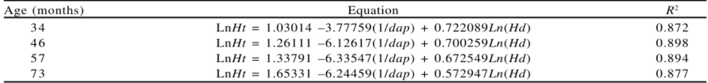
The model LnHt = β0 + β1/dbh + β2LnHd + ε (3) was fitted with data of each measurement from the 25 permanent fixed- and variable-area plots, where Hd
is the mean dominant height of the plot. The equations obtained were used to estimate the trees that had only the dbh measurement in each type of plot.
The equations obtained by the fit of the models (1), and (2), and (3) were used to process the fixed-area and variable-fixed-area plots.
The volume and basal area estimates obtained for each year, with fixed and variable-area plots, were compared using the procedure proposed by Leite and Oliveira (2002). A synthesis of this procedure is presented in the Appendix.
To obtain the site index of each plot, the dominant height and age data were used to fit the Richards model as follows:
(4)
where Hd is the mean dominant height of the plot
in meter, and I is the age, in months.
Specific site index equations were not generated for variable area methodology because the variable-area plots were in the same locations as the fixed-variable-area plots, resulting in the same guide-curve. The age index adopted was 60 months.
To estimate growth and yield for each type of plot, the models including the variables I, I and S,
and I, S and B were fitted. The models were adjusted
for volume (V) and mass (W) with bark up to a minimum
commercial diameter of 4.0 cm using the Quasi Newton procedure, except for the Clutter model , V=f(I,S,B),
fitted by the two stages least squared method. The models fitted were
(5)
(6)
(7a)
(7b)
where:
Y2 = volume, m3ha-1 or mass, kgha-1, at the future age I2;
I1 and I2 = current and future ages, in months;
B1 and B2 = current and future basal areas, in m3ha-1;
S1 = site index at the current age, m;
bi = regression parameters;
e = random error, ;
Ln = neperian logarithm base.
Growth and yield curves were constructed with the equations obtained from the fixed and variable-area plot data and the technical rotation was determined for each case. The estimates of yield in wood volume and mass obtained with the two data sources were compared using the procedure proposed by Leite and Oliveira (2002).
3. RESULTS AND DISCUSSION
Age Statistic Total Quadratic Basal area Volume Mass (months) heigth (m) diameter (cm) (m2ha-1) (m3ha-1) (kg.ha-1)
F V F V F V F V F V
34 Mean 10.8 11.5 8.1 9.2 5.98 7.24 28.98 34.74 12697.342 15587.13
34 Standard deviation 1.9 2.1 0.9 1.4 1.88 2.14 14.13 16.31 6156.05 6958.63 34 Standard error 0.4 0.4 0.2 0.3 0.38 0.43 2.83 3.26 1231.21 1391.73 34 Sampling error (%) 7.2 7.4 4.7 6.4 12.93 12.18 9.75 9.39 9.70 8.93 46 Mean 13.3 14.5 10.4 11.7 9.68 9.76 62.76 62.97 27553.02 23087.70 46 Standard deviation 2.3 2.4 1.1 1.3 2.02 2.89 22.94 25.65 9947.77 9559.96 46 Standard error 0.5 0.5 0.2 0.3 0.40 0.58 4.59 5.13 1989.55 1911.99 46 Sampling error (%) 7.1 7.0 4.2 4.5 8.58 12.19 15.06 16.78 14.87 17.06 57 Mean 15.5 17.1 11.7 13.5 14.02 14.04 108.55 108.87 47567.39 47737.25 57 Standard deviation 2.4 2.7 1.1 1.4 2.79 3.54 36.92 39.67 15985.16 17243.89 57 Standard error 0.5 0.5 0.2 0.3 0.56 0.71 7.38 7.93 3197.03 3448.78 57 Sampling error (%) 6.4 6.4 3.8 4.2 8.21 10.38 14.01 15.01 13.85 14.88 73 Mean 17.5 19.2 12.5 14.2 16.12 17.00 144.22 148.97 62973.83 65002.61 73 Standard deviation 2.3 2.5 1.2 1.5 3.45 4.07 48.99 48.78 21221.29 21129.83 73 Standard error 0.5 0.5 0.2 0.3 0.69 0.81 9.80 9.76 4244.26 4225.97 73 Sampling error (%) 5.4 5.3 3.9 4.2 8.83 9.86 14.00 13.49 13.88 13.39
Table 2 – Statistics obtained using fixed-area plot (F) and variable-area plot (V), with basal area factor k = 1 Tabela 2 – Estatísticas obtidas usando parcela de área fixa (F) e de área variável (V), com fator de área basal k = 1
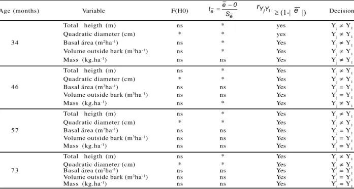
The total height and quadratic diameter measurements obtained with the fixed- and variable-area plot were significantly different (p < 0.05) by the statistical procedure proposed by Leite and Oliveira (2002) (Table 3). Similar results were reported by Couto et al. (1993) in a temporary inventory conducted in a four-year-old Eucalyptus saligna stand. Basal area statistics were statistically equal after 46 months, by the same statistical procedure (p > 0.05). Except for the first volume measurement and the second mass measurement, the wood volume and mass measurements obtained with the two types of plots were statistically equal (p > 0.05).
Generally, it can be inferred that both types of plots can be used to estimate basal area, wood volume and mass at consecutive ages, that is, for continuous forest inventory. Although the precision of the inventory was not assessed, when interpreting the confidence intervals for wood volume and mass, implicit in Table 2, it was found that both intervals contained the means
obtained with the two types of plots, at 46, 57 and 73 months.
3.1. Growth and yield modeling
The equation obtained to estimate the dominant height with determination coefficient (R2) equal to 0.736 was:
Considering the functional relationship above and that the site index is the dominant height at the index age (60 months), it results in:
and
Age (months) Equation R2
3 4 LnHt = 1.03014 –3.77759(1/dap) + 0.722089Ln(Hd) 0.872 4 6 LnHt = 1.26111 –6.12617(1/dap) + 0.700259Ln(Hd) 0.898
5 7 LnHt = 1.33791 –6.33547(1/dap) + 0.672549Ln(Hd) 0.894 7 3 LnHt = 1.65331 –6.24459(1/dap) + 0.572947Ln(Hd) 0.877
Table 1 – Height equations for Eucalyptus stands in high bole system in the Central Western Region of Minas Gerais, Brazil Tabela 1 – Equações de altura para povoamentos de eucalipto em sistema de toras longas na Região Centro-oeste de Minas
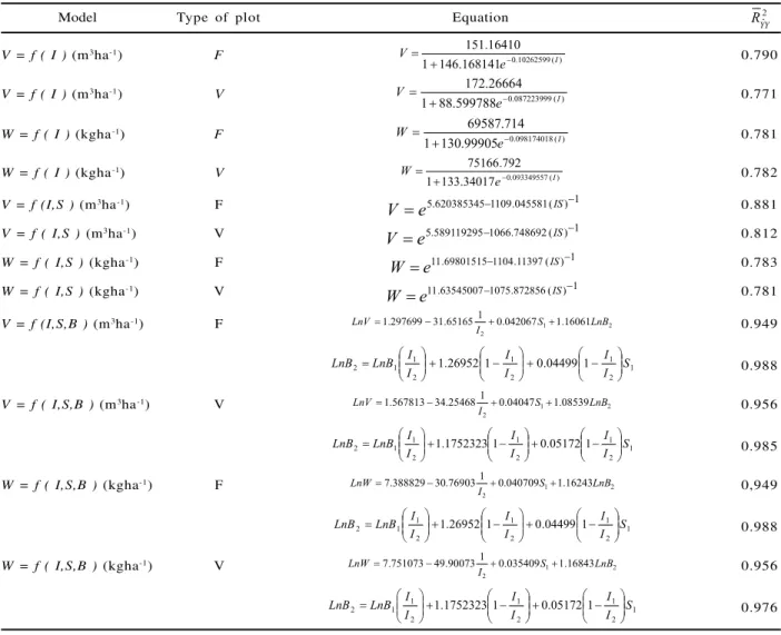
These expressions were used to generate the anamorphic site index curves (Figure 1) and the site indexes per plot. Table 4 shows the growth and yield models fitted with the fixed- area and variable-area plot data.
Residual analyses do not indicate bias. However, more precise estimates were obtained with the V=f(I,S,B)
model type, as expected. This type of model is frequently used for eucalyptus and pine plantations in Brazil.
Using the equations V=f(I,S,B) and W=f(I,S,B), Table 4, the technical rotations were determined for the site indexes 28, 22 and 16, considering the mean initial basal areas observed at 34 months. The rotation did not differ greatly when one or the other plot type was adopted (Table 5). This indicates that the variable-area plots can in principle be used in growth and yield modeling. The rotations were obtained by -β1 S-1 for the models V=f(I,S) and W=f(I,S); the models V=f(I) and W=f(I) were those corresponding to the maximum mean monthly increase. Except for model W=f(I,S,B), the rotations indicated in Table 5 are in line with the expectations for the species and region where the stands were located.
Age (months) Variable F(H0) Decision
Total heigth (m) ns * yes Yj ≠ Y1
Quadratic diameter (cm) * * yes Yj ≠ Y1
3 4 Basal área (m2ha-1) ns * Yes Y
j ≠ Y1
Volume outside bark (m3ha-1) ns * Yes Y
j ≠ Y1
Mass (kg.ha-1) ns ns Yes Y
j ≠ Y1
Total heigth (m) ns * Yes Yj ≠ Y1
Quadratic diameter (cm) * * Yes Yj ≠ Y1
4 6 Basal área (m2ha-1) ns ns Yes Y
j = Y1
Volume outside bark (m3ha-1) ns ns Yes Y
j = Y1
Mass (kg.ha-1) ns * Yes Y
j ≠ Y1
Total heigth (m) ns * Yes Yj ≠ Y1
Quadratic diameter (cm) * * Yes Yj ≠ Y1
5 7 Basal área (m2ha-1) ns ns Yes Y
j = Y1
Volume outside bark (m3ha-1) ns ns Yes Y
j = Y1
Mass (kg.ha-1) ns ns Yes Y
j = Y1
Total heigth (m) ns * Yes Yj ≠ Y1
Quadratic diameter (cm) * * Yes Yj ≠ Y1
7 3 Basal área (m2ha-1) ns ns Yes Y
j = Y1
Volume outside bark (m3ha-1) ns ns Yes Y
j = Y1
Mass (kg.ha-1) ns ns Yes Y
j = Y1 Yj and Yi indicate estimates obtained with variable- and fixed-area plots, respectively. ns = p> 0.05 and * = p< 0.05.
Table 3 – Results of the L&O procedure applied to compare the estimates of mean total height, mean diameter, basal area, wood volume and mass, at different ages *
Tabela 3 – Resultados do procedimento L&O utilizado para comparar as estimativas de altura total média, diâmetro médio, área basal, volume e massa de madeira e, em idades diferentes *
Figure 1 – Site index anamorphic curves for even-aged Eucalyptus
stands in the central western region of Minas Gerais State, Brazil. (Index age = 60 months). Figura 1 – Curvas anamórficas de índices de local para
The model L n B34=β0+β1S+ε was fitted to simulate growth and yield using the Clutter model,
V=f(I,S,B) and W=f(I,S,B) from different site indexes
and initial basal areas, using data from the first measurement of the permanent plots, resulting in LnB34 = -0,068004289 + 0,088872711(S) with r
2
= 0.691 and B34, the basal area at 34 months. Although statistically equal (Table 6), the difference among volume estimates increase with the decrease in the site index (Figure 2). The yield curves are coincident from the 24 m site index. The greatest
differences detected when the W=f(I,S,B) model was adopted may have occurred because of the worse fit found for this model when variable-area plots were adopted to estimate mass (Table 4).
The statistical procedure proposed by Leite and Oliveira (2002) was also used to compare the models generated with data from fixed and variable area plots. For this purpose, volume and mass estimates were generated for the site index and basal area recorded at the first measurement (34 months). Wood volume and mass were projected from these data for the ages
Model Type of plot Equation
V = f ( I ) (m3ha-1) F 0.790
V = f ( I ) (m3ha-1) V 0.771
W = f ( I ) (kgha-1) F 0.781
W = f ( I ) (kgha-1) V 0.782
V = f (I,S ) (m3ha-1) F 0.881
V = f ( I,S ) (m3ha-1) V 0.812
W = f ( I,S ) (kgha-1) F 0.783
W = f ( I,S ) (kgha-1) V 0.781
V = f (I,S,B ) (m3ha-1) F 0.949
0.988
V = f ( I,S,B ) (m3ha-1) V 0.956
0.985
W = f ( I,S,B ) (kgha-1) F 0,949
0.988
W = f ( I,S,B ) (kgha-1) V 0.956
0.976
Table 4 – Growth and yield models, in wood mass and volume, fitted with data from fixed-area and variable-area plots considering different independent variables
46, 57 and 73 months. These estimates were then compared (Table 6). Significant difference was only detected for wood mass, using the models V=f(I,S,B) and w=f(I,S,B). The volume estimates generated by the
model V=f(I,S) for site indexes 16, 22 and 26 were coincident (Figure 3). Therefore, it can be inferred that permanent sampling point can be used for growth and yield modeling.
Figure 2 – Yield curves for even-aged Eucalyptus stands in the Central Western Region of Minas Gerais, Brazil, obtained with the Clutter model fitted with data from fixed- and variable-area plots.
Model Site index (m) Fixed-area plot Permanent sample point
Volume Mass Volume Mass
2 8 6 3 6 3 6 6 8 5
2 2 6 4 6 3 6 6 8 4
V = f(I,S,B) 1 6 6 8 6 7 6 8 8 7
2 8 4 0 3 9 3 8 3 8
V = f(I,S) 2 2 5 0 5 0 4 8 4 9
1 6 6 9 6 9 6 7 6 7
2 8 6 6 6 7 7 0 7 1
V = f(I) 2 2 6 6 6 7 7 0 7 1
1 6 6 6 6 7 7 0 7 1
Table 5 – Rotation in months obtained from the models V=f(I,S,B), V=f(I,S) and V=f(I), for wood volume and mass, for site index 28, 22 and 16 m
Tabela 5 – Rotação em meses obtida dos modelos V=f(I,S,B), V=f(I,S) e V=f(I), para volume e massa de madeira, para índices de local 28, 22 e 16 m
Figure 3 – Growth curves (m3ha-1 and t.ha-1) for even-aged Eucalyptus stands in the Central Western Region of Minas Gerais, Brazil, using models of the V=f(I) and V=f(I,S) fitted with data from fixed- and variable-area plots.
Figura 3 – Curvas de crescimento (m3ha-1 e t.ha-1) para povoamentos homogêneos de Eucalipto na Região Centro-oeste
de Minas Gerais, Brasil, usando modelos de V=f(I) e V=f(I,S) ajustados com dados de parcela de área fixa e variável.
Model Variable F(H0) Decision
V = f(I,S,B) Volume (m3ha-1) ns ns yes Y
j = Y1
V = f(I,S,B) Mass (t.ha-1) * * yes Y
j ≠ Y1
V = f(I,S) Volume (m3ha-1) ns ns yes Y
j = Y1
V = f(I,S) Mass (t.ha-1) ns ns yes Y
j = Y1
V = f(I) Volume (m3ha-1) ns ns yes Y
j = Y1
V = f(I) Mass (t.ha-1) ns ns yes Y
j = Y1
ns = p>0.05 and * = p< 0.05.
Table 6 – L&O test applied to compare the models fitted with fixed-area (Y1) and variable-area (Yj) plots
4. CONCLUSIONS
Based on the results it can be concluded:
- permanent sampling point are efficient to conduct continuous forest inventories;
- data obtained from permanent sampling points are efficient for growth and yield modeling at stand level;
- the Bitterlich method enables precise and umbiased estimates of basal area, volume and mass per hectare in eucalyptus plantations, at different ages;
Although it was not the objective to study regular mortality, it can be inferred that the use of permanent sampling points does not hinder its quantification. Quantification can be carried out between any two ages if only the trees classified on the first of these two occasions is considered.
5. REFERENCES
AVERY, T.E. Gross volume estimation using “plotless cruising” in Southern Arkansas.
Journal. Forest, v.53, p.206-207, 1955.
BELL, J.F.; ALEXANDER, L.B. Application of the variable plot method of sampling forest stands.
Oregon State Board Forestry Research, Note 30, 22 p., Illus.1967.
CAMPOS, J.C.C. Aplicação de um modelo compatível de crescimento e produção de densidade variável em plantações de
E u c a l y p t u s g r a n d i s. Revista Árvore, v.2, n.10, p.121-134,1986.
CAMPOS, J.C.C.; SILVA CAMPOS, A.L.A.; LEITE, H.G. Decisão silvicultural empregando um sistema de predição do crescimento e da produção.
Revista Árvore, v.12, n.2, p.100-110, 1988.
CAMPOS, J.C.C.; RIBEIRO, J.C. Efeito da qualidade de local na rotação técnica de eucalipto. Revista Árvore, v.11, n.2, p.146-157, 1987.
CAMPOS, J.C.C.; LEITE, H.G. Mensuração florestal: perguntas e respostas. Editora UFV, Universidade Federal de Viçosa, 2002. 407 p.
COUTO, H.T.Z.; BASTOS, N.L.M.; LACERDA, J.S. A amostragem por pontos na estimativa de área basal em povoamentos de Eucalyptus. IPEF, v.46, p.86-95, 1993.
GRAYBILL, F. A. Theory and application of the linear model. Massachusetts: Duxburg Press, 1976. 704p.
GROSENBAUGH, L.R. Point-sampling a n d l i n e - s a m p l i n g: p r o b a b i l i t y t h e o r y, geometric implications, synthesis ocasional. Washington: USDA, Forest Service, 1952. 34p. (Paper, 160).
GROSENBAUGH, L.R; STOVER, W.S. Point-samplig compared with plot-sampling in southeast Texas. Forest Science, v.3. p.3-14, 1957.
GUIMARÃES, D.P. Desenvolvimento de um modelo de distribuição diamétrica de passo invariante para prognose e projeção da estrutura de povoamentos de eucalipto. 1994. 160f. Tese (Doutorado em Ciência Florestal) – Universidade Federal de Viçosa, Viçosa, MG, 1994.
HIRATA, T. Heigth estimation through Bitterlich´s method vertical angle-count s a m p l i n g . J a p a n e s e J o u r n a l F o re s t r y, v.37, p.479-480, 1955.
KIRBY, C.L. Accuracy of point sampling in white spruce-aspen stands. Sasktchewan Journal Forest, v.63, n.12, p.924-926, 1965.
LEITE, H.G. Ajuste de um modelo de estimação de frequência e produção por classe de diâmetro, para
povoamentos de Eucalyptus saligna Smith.
1990. 78f. Dissertação (Mestrado em Ciência Florestal) – Universidade Federal de Viçosa, Viçosa, MG, 1990.
LEITE, H.G.; OLIVEIRA, F.L.T. Statistical procedure to test the identity of analytical methods.
Communications in Soil Science and Plant Analysis, v.33, p.7-8, 2002.
LEITE, H.G.; GUIMARÃES, D.P.; CAMPOS, J.C.C. Descrição e emprego de um modelo para estimar múltiplos volumes de árvores. Revista
LISITA, A. Efeitos de reespaçamentos no crescimento e na produção de
povoamentos de Eucalyptus camaldulensis
Procedência Petford. 1997. 70 f. Dissertação (Mestrado em Ciência Florestal) - Universidade Federal de Viçosa, Viçosa, MG, 1997.
NOGUEIRA, G.S. et al. Determinação da idade técnica de desbaste em plantações de eucalipto utilizando o método dos ingressos percentuais.
Scientia Forestalis, n.59, p.51-59, 2001.
NOGUEIRA, G. S. Modelagem do
crescimento e produção de povoamentos de Eucalyptus sp. e de Tectona grandis
submetidos a desbaste. 146f. Tese (Doutorado em Ciência Florestal) – Universidade Federal de Viçosa, Viçosa, MG, 2003.
ROSAS, M.P. Alternativas de
determinação da idade técnica de corte de Eucalyptus urophylla. 1994. 70f. Dissertação (Mestrado em Ciência Florestal) -Universidade Federal de Viçosa, Viçosa, MG, 1994.
SILVA, A.A.L. Emprego de modelos de crescimento e produção em análise econômica de decisões de manejo florestal. 2001. 69f. Tese (Doutorado em Ciência Florestal) – Universidade Federal de Viçosa, Viçosa, MG, 2001.
SILVA, L.B.X. Tamanho e forma de unidades de amostra em amostragem aleatória e sistemática para florestas plantadas em
E u c a l y p t u s a l b a Rewien. Revista
Floresta, v.8. n.1, p.13-18, 1977.
SOARES, C.P.B. Um modelo para o gerenciamento da produção de madeira em plantios comerciais de eucalipto. 1999. 71f. Tese (Doutorado em Ciência Florestal) – Universidade Federal de Viçosa, Viçoa, MG, 1999.
S O U Z A , A . L . C o m p a r a ç ã o d e t i p o s d e a m o s t r a g e n s , c o m p a r c e l a s
c i r c u l a r e s d e á r e a f i x a e v a r i á v e l , e m p o v o a m e n t o s d e E u c a l y p t u s g r a n d i s
d e o r i g e m h í b r i d a , c u l t i v a d a s n a r e g i ã o d e B o m D e s p a c h o , M i n a s Gerais.1981. 79f. Dissertação (Mestrado em Ciência Florestal) – Universidade Federal de Viçosa, Viçosa, MG, 1981.
STRAND, L. Relaskopik hoyde- og
kubikkmassebestemmelse. Norsk Skogbruk, v.3, p.535-538, 1957.
THOMSON, G.W.; DEITSCHMAN, G.H.
APPENDIX
The procedure proposed by Leite and Oliveira (2002) named L&O test, consists of a decision rule constructed on the basis of the F statistic proposed by Graybill (1976) for the assessment of the mean error and the analysis of the coefficient of linear correlation among two quantitative data vectors. According to the authors, y1 and yj are two vectors of quantitative data, where j indicates an alternative method, procedure or treatment and 1 the standard treatment. The relationship between y1 and yj can be expressed matrixically by Yj=Y1β+ε , where Yj = yj and Yj =[y1∅], ∅ = [1 …1].
Under normality, , where
is the mean square of the residues of the simple linear regression: Yj = Y1β+ ε. Thus, with n-2 degrees
of freedom and a level of significance α, the F statistic is used to assess the hypothesis H0: β’ = [0 1]. If F(H0) ≥Fa (2, n-2 g.l.) H0 is rejected, on the contrary H0 is accepted.
Considering that the errors ei = (Yji - Y1i)/Y1i follow
normal distribution, the H0: hypothesis vs Ha: not H0 can be tested using the t statistic, given by
and with n-1 degrees of freedom. If ≥
tα(n-1 g.l.) the H0 hypothesis is rejected; on the contrary H0 is accepted.