ABSTRACT: The main purpose of this study was to assess nonlinear models generated by in-tegrating the basal area growth rate to estimate the growth and yield of forest stands. The database was collected from permanent sample units, in Paraopeba county, in the state of Minas Gerais, Brazil. The stands were represented by Eucalyptus camaldulensis × Eucalyptus urophylla hybrid trees, with 3 × 3 meters of spacing. The data were divided into two groups: fit-ting and validafit-ting databases. Two nonlinear models (Strategy A and Strategy B) were developed using differential equations to estimate the basal area growth and yield of the sample units. The logistic model was fitted to estimate the volumetric yield as a function of age, site index and basal area. The efficiency of the systems generated by logistic model and models obtained by differential equations (Strategy A and Strategy B) was also compared to the efficiency of the system estimated by the Clutter model (Strategy C). The projection models used to estimate basal area obtained by differential equations were compatible with forest growth and yield, and the logistic model with covariates was compatible with volumetric growth and yield. Strategy A and Strategy B generated different thinning and harvesting options for different site indices, which is biologically consistent.
Keywords: nonlinear models, compatible models, biological consistency
Growth and yield models for eucalyptus stands obtained by differential equations
Adriano Ribeiro de Mendonça1*, Natalino Calegario2, Gilson Fernandes da Silva1, Samuel de Pádua Chaves e Carvalho3
1Federal University of Espírito Santo – Dept. of Forest and Wood Science, Av. Governador Lindemberg, 316 – 29550-000 – Jerônimo Monteiro, ES – Brazil.
2Federal University of Lavras – Dept. of Forest Science, C.P. 3037 – Campus Universitário – 37200-0000 – Lavras, MG – Brazil.
3Federal University of Mato Grosso/Faculty of Forest Engineering – Dept. of Forest Engineering, Av. Fernando Correa da Costa, 2367 – 78060-900 – Cuiabá, MT – Brazil. *Corresponding author <[email protected]>
Edited by: Rafael Rubilar Pons
Received January 24, 2016 Accepted September 11, 2016
Introduction
An accurate estimation of forest growth and yield is fundamental to the achievement of forestry planning objectives. The stand growth and yield volume, both present and future, are the most important items of in-formation if forestry planning is to be successful.
Moreover, an important positive in growth and yield studies is the opportunity to implement prognosis models. Growth models represent the relationship between the quantity of yield and growth and the various factors that explain or allow for the estimation of this growth (Davis et al., 2000) and several studies on forest growth and yield have been completed in the past including the following: Bonet et al. (2012), Burkhart (1971), Clutter (1963), Pi-enaar (1979), PiPi-enaar and Turnbull (1973), Schumacher (1939) and Sullivan and Clutter (1972).
The sampling process for estimating the present yield of forest stands and their dynamics has led to the continued improvement of techniques used to construct growth and yield models. Growth models can be repre-sented by differential equations or by systems with two or more differential equations (Wraith and Or, 1988). Clutter (1963) and Schumacher (1939) have used differential equa-tions in their models, but most of them have used linear relationships only. Furthermore, Garcia (1980) developed a stochastic differential equation model for the height growth of even-aged stands in which the deterministic part is equivalent to the Bertalanffy-Richards model.
By using nonlinear models, important assump-tions are incorporated in the problem of obtaining a the-oretical relationship between the variables of interest, instead of an empirical description. Another advantage of nonlinear models lies in parameter interpretation and parsimony. In many situations, nonlinear models require
fewer parameters than linear models, which can sim-plify the interpretation of the model results. Nonlinear yield models, with sigmoidal trend lines, represent the growth of individuals, or populations by presenting the same trend line of the yield over time. Examples using models to project growth by nonlinear equations are Koya and Goshu (2013) and Zeide (1993, 2004). In a uni-fied sigmoid growth equation, Garcia (2005) states that a general model can simplify the study of properties such as the presence and nature of asymptotes and inflection points, and facilitate the development of more widely applicable software.
In this context, the main objective of the present study was to model basal area differential equations in order to generate nonlinear models that can estimate the growth and yield of forest stands.
Materials and Methods
Study area and databaseThe database used in this study was obtained from an area located in Paraopeba county (19º16’28” S, 44º24’15” W and altitude of 761m), in the state of Minas Gerais, Brazil. The average temperature in this region is 20.9 °C, the annual mean precipitation 1328 mm.
Development of the growth and yield models The approach used in this study is quite different from that taken by Clutter (1963). In this study the de-pendent variable was not transformed and the growth function used had a nonlinear parameter combination. Two modeling strategies were developed (Strategies A and B). When implementing Strategy A, the first step was to choose a model that represented variations of the current annual increment (CAI) over time. The model chosen was Y =β A e−βX
0 1
. (1) (Ratkowsky, 1990). Considering the methodology proposed by Clutter (1963) for linear approach and the expression (1), wherein Y is equal to the CAI in basal area of the stand and X is equal to the age of the stand, it is possible to compose the fol-lowing expression for CAI:
CAI dB
dA Ae
A
= =β −β
0
1 (2)
wherein B = basal area of ith stand (m² ha−1), A = age of the stand (years), βi = parameters of the model and e = base of the natural logarithm.
Expression (2) is a separable differential equation and was integrated to obtain a basal area yield function:
dB= Ae− AdA
∫
∫
β β0 1
B e A e
A A =
(
− −)
− − β β β β β 0 1 1 2 1 1 (3)The projection model for the basal area of the stand was derived by integrating equation (2) from basal areas B1 to B2 and from ages A1 to A2:
dB Ae dA
B B A A A 1 2 1 1 2 0
∫
=∫
β −βB B e A e A
A A
2 1 0
1 2 1 1
1 2
1 2 1 1 1 1
− = −
(
+)
+(
+)
− −β β β
β
β β
B B e A e A
A A
2 1 0
1 2 1 1
1 2
12 1 1 1 1
= + −
(
+)
+(
+)
− −β β β
β
β β
(4)
wherein B1 = basal area for age A1, B2 = basal area for age A2, A1 = present age, and A2 = future age.
The basal area also depends on the stand site quality. Next, in expression (4) the effect of the site in-dex was incorporated (S) as a covariate (Guimarães et al., 2009):
B B S e S A e
A
2 1 00 01
10 11 2
10 11 2 1 10 11
= =( + ) − ( + ) + +
−( + ) − +
β β β β
β β β β SS A
S A S ( ) ( + ) + + ( ) 1
10 11 1 10 11 2 1 β β β β (5)
The next step was to choose a model to estimate the stand volume. The logistic model was used to esti-mate volumetric yield:
V
e A
2 0
1 1 2 2
=
+ ( − ) +
β ε
β β (6)
wherein V2 = the stand volume for age A2, and ε = sto-chastic error.
The logistic model, like other nonlinear models, can be fitted using the initial parameter values generated by interpreting them. The parameter β0represents the upper horizontal asymptote (UHA); specifically, the maximum response value (V2) as time tends to +∞. The parameter β1represents the inflexion point of the curve; in other words, the age (A2) where the yield (V2) reaches half of β0.The parameter β2 represents the difference between the age when the yield reaches approximately 73 % of β0 and the age corresponding to the inflexion point. This interpretation is very useful, as the greatest limitation in using nonlinear models is the correct choice of initial parameters for the iteration process. Based on the fact that the variation of the total stand volume is explained by more than their age, the parameters of the logistic model were decomposed inserting the site index (S) and the basal area of the stand (B) as covariates (ex-pression 7).
V S B
e S B A S B
2
00 01 01 2
1 10 11 12 2 2 20 21 22 2
= + +
+ ( + + )− ( + +
β β β
β β β β β β ))
{ }+ ε (7)
To test the compatibility of the logistic model with covariates, the first derivative of the growth function was solved as a function of age.
To develop Strategy B, the expression (1) was re-placed by the following CAI expression (Ratkowsky, 1990):
CAI dB
dA A e
A
= =
(
β −β)
−β0 1
0 (8)
The replacement of the expression (1) by expres-sion (8) is the only difference between Strategies A and B, i.e., the other steps are the same. Considering that the Clutter model is widely used in forest studies, Strate-gies A and B were compared to his model. To simplify the result interpretations, the Clutter model was called Strategy C. In summary, we had the following systems of equations for Strategies A, B and C:
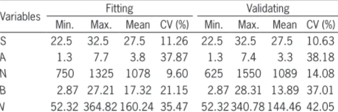
Table 1 − Descriptive statistics of variables related to stands of the
Eucalyptus camaldulensis × Eucalyptus urophylla.
Variables Fitting Validating
Min. Max. Mean CV (%) Min. Max. Mean CV (%)
S 22.5 32.5 27.5 11.26 22.5 32.5 27.5 10.63
A 1.3 7.7 3.8 37.87 1.3 7.4 3.3 38.18
N 750 1325 1078 9.60 625 1550 1089 14.08
B 2.87 27.21 17.32 21.15 2.87 28.31 13.89 37.01 V 52.32 364.82 160.24 35.47 52.32 340.78 144.46 42.05 Wherein: S = site index (m); A= age (years); N= number of trees per hectare (trees ha−1)
; B = basal area (m
Strategy A:
B B S e S A e
A
2 1 00 01
10 11 2
10 11 2 1 10 11
= =( + ) − ( + ) + +
−( + ) − +
β β β β
β β β β SS A
S A S ( ) ( + ) + + ( ) 1
10 11 1 10 11 2 1 β β β β (5)
V S B
e S B A S B
2 00 01 01 2
1 10 11 12 2 2 20 21 22 2
= + +
+ ( + + )− ( + +
β β β
β β β β β β ))
{ }+ ε (7)
Strategy B:
B B
e S A S
e
S A
2 1
00 01 2 10 11
00 01 2
00 1 = + −
(
+)
− +(
+)
+ − + − + ( ) ( β β ββ β β β
ββ β β β β
β β
01 1
00 01 1 10 11
00 01
1
S A
S A S
S )
(
+)
+ −(
+)
+(
)
(9)V S B
e S B A S B
2
00 01 01 2
1 10 11 12 2 2 20 21 22 2
= + +
+ ( + + )− ( + +
β β β
β β β β β β ))
{ }+ ε
(7)
Strategy C:
LnV
A S LnB
2 0 1
2
2 3 2
1 = + + + +
β β β β ε (10)
LnB LnB A
A
A A
A
A S
2 1 1
2 0 1 2 1 1 2 1 1 = + − + − +
α α ε (11)
wherein Ln = natural logarithm, and αi = parameters of the model.
The stand’s basal area projection and volume models were fitted by R statistical software (Version 2.10.1). The projection models of Strategies A and B (expressions 5, 7 and 9) were fitted using the nlme
package. The Clutter model (expressions 10 and 11) was fitted using the least squares method in two stages (systemfit package).
Evaluation of the models
To compare the models evaluated in terms of ac-curacy, the following statistics were applied:
a)R2as proposed by Kvalseth (1985)
R Y Y Y Y i i i n i i n 2 2 1 2 1 1 = − −
(
)
−(
)
= =∑
∑
ˆR R n
n p
2= −1
(
1− 2)
(
−1)
−
wherein R2= adjusted coefficient of determination;
R² = coefficient of determination, n = number of observations, p = number of parameters. Yˆ
i = the
estimated values of stand basal area or volume by the model, Yi = observed values of stand basal area or volume,Y= average of the stand basal area or volume.
b) Root mean square error:
RMSE Y Y n p i i i n = =
(
)
− =∑
ˆ 1 2 RMSE RMSE Y(%)= 100
wherein RMSE = root mean square error.
c) Bias B Y Y n i i n i i n = − = =
∑
∑
1 1 ˆ B B Y %( )
=100wherein B = bias.
Furthermore, error graphical analyses (%) were performed to check the quality of the model estimations. The values of the error (%) used in the construction of the graphs were expressed by:
i i i i Y Y Error Y ˆ
(%)=100 − .
Results and Discussion
Analysis of the growth and yield modelsTable 2 presents the statistics corresponding to the fit of the basal area projection considering Strategies A, B and C.
The parameter α1of Clutter’s system of equations was removed from the model because it was not signifi-cant (p-value > 0.05). In terms of the root mean square error [RMSE (%)], Strategy B had a better performance, followed by Strategies A and C. The results were similar using the statistical R2and Bias (%), with Strategy B per-forming better than either Strategy A or C.
The results in Table 2 show that Strategies A, B and C presented similar performance in projecting the basal area with a slight advantage for Strategy B. On the
Table 2 − Statistics for the basal area projection models for the stands for the fit data.
Strategy A (R2= 0.9255; RMSE % = 5.69 %; Bias (%) = 0.55 %)
Parameter Estimate Standard error t p-value
β00 25.64821 5.38068 4.77 < 0.001
β01 -0.54550 0.18440 -2.96 0.004
β10 1.13779 0.16258 7.00 < 0.001
β11 -0.01382 0.00590 -3.02 0.003
Strategy B (R2 = 0.9349; RMSE % = 5.32; Bias (%) = 0.24 %)
Parameter Estimate Standard error t p-value
β00 0.85473 0.14296 5.98 < 0.001
β01 -0.01830 0.00520 -3.52 < 0.001
β10 -28.08757 5.19361 -5.41 < 0.001
β11 0.60196 0.17786 3.38 < 0.001
Strategy C (R2= 0.9229; RMSE %= 5.85; Bias (%) = -0.29 %)
Parameter Estimate Standard error t p-value
α0 3.564632 0.03804 93.69 < 0.001
other hand, if the basal area databases, from forest inven-tory, are available and it is not necessary to project this variable, it is possible to compare the volumes projected by Strategies A and B with the volume projected by the Clutter model. As Strategies A and B used the same expres-sion to project the volume, i.e., the Logistics model, a com-parison was then made between this model and Clutter’s volumetric model (Table 3).
However, when comparing the logistics model (ex-pression 7) with the Clutter model (ex(ex-pression 10), a num-ber of inconsistent results were found; for example, lower cutting ages in less productive sites. Thus, expression 7 was rearranged by testing different combinations of S and B2 as covariates in order to find consistent results. The combina-tion of S and B2 that best met consistent results is presented in Table 3.
All of the parameters were significant (p-value < 0.001). The models evaluated showed accurate volumetric growth and yield estimates (RMSE < 4 % and R2 > 0.98) and the Clutter model performed slightly better than the logistics model. This indicates that both models can be used for estimating stand volume. However, the logistics model presented smaller Bias (%) and often this is the model of choice.
Compatibility of the logistics model with covariates in estimating the volumetric yield
The compatibility of the logistic model was tested by taking the first derivative of the yield model as a func-tion of age:
∂ ∂ =
+
+
{
( + )− }
V A
S
e
i
i Bi Ai
ˆ ˆ
ˆ ˆ ˆ
β β
β β β
00 01
1 10 11 2
(12)
The basal area was estimated for Strategy B (9), site index of 20 m and ages from 2 to 4 years old. The basal area estimated for 2 years old was equal to 2.50 m2 ha–1. After integrating the growth equation, the yield estimated
was 25.35 m3 ha–1. For three years old, the basal area was 7.65 m2 ha–1 and the yield was 43.82 m3 ha–1. For four years old, the basal area was 11.03 m2 ha–1 and the yield was 74.66 m3 ha–1. The same yields were obtained using equa-tion (7), demonstrating the compatibility of the proposed estimation process.
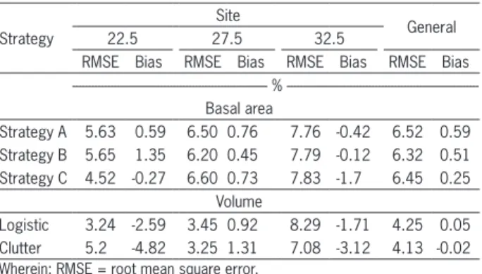
Analysis of validation data of growth and yield models for calculating basal area and volume
Table 4 shows the RMSE (%) and the Bias (%) of the growth and yield projection used to estimate stand basal area (Strategies A, B and C) and volume. The comparison of the volumetric models was made in the same way to produce the results in Table 3.
In general, the models showed to be accurate when estimating basal area (RMSE < 8 % and Bias < 1.5 %) and volume (RMSE < 9 % and Bias < 5 %) in all sites. The results obtained with the validation data were similar to those obtained with the data used for fitting the models.
The residual distributions estimated with the basal area projection models are shown in Figure 1. Most errors were concentrated within the range of ± 10 % (Figure 1). Despite this, the models had a certain tendency to underes-timate the stand basal area located above 25 m2 ha−1. The range of stand basal area observed, approximately from 8.1 to 28.3 m² ha−1, was the same as estimated by both the proposed and the Strategy C models.
The residual distribution for the logistic model with covariates and the Clutter model for volumetric growth and yield estimates is shown in Figure 2. The majority of errors were ± 10 %. The low error from Figure 2 is in agree-ment with the low value of RMSE as reported in Table 4.
Table 5 shows the RMSE (%) and Bias (%) for the strategies’ stand volume projections.
The results (Table 5) demonstrated that the strategies were accurate and similar to estimate stand volume. When comparing the RMSE values (%), Strategy B presented the best volume projection result followed by Strategy A and Strategy C in all sites. But, when comparing the value of Bias (%), the best result was obtained when using Strategy C. Table 3 − Statistics of the logistics model with addition of covariates
and statistics of the Clutter model to estimate volumetric growth and yield for the fit data.
Logistic with Covariates (R2=0.9881; RMSE % = 3.80; Bias (%) = -0.03)
Parameter Estimate Standard error t p-value
β00 218.65999 23.50651 9.30 < 0.001 β01 S 10.83302 0.73223 14.79 < 0.001
β10 27.06476 1.76727 15.31 < 0.001
β11B2 -0.91066 0.06159 -14.79 < 0.001
β2 8.30707 0.52370 15.86 < 0.001 Clutter (R2= 0.9890; RMSE % = 3.68; Bias (%) = 0.22)
Parameter Estimate Standard error t p-value
β0 1.40134 0.07886 17.77 < 0.001
β1 -1.53391 0.07412 -20.69 < 0.001
β2 0.02136 0.00111 19.18 < 0.001
β3 1.20767 0.02577 46.86 < 0.001
Wherein: R2
= adjusted determination coefficient; RMSE= root mean square error; S = site index (S) and B2 = basal area for age A2.
Table 4 − Root mean square error [RMSE (%)] and relative bias [Bias (%)] for growth and yield projection models used to estimate the basal area and volume of Eucalyptus camaldulensis × Eucalyptus
urophylla stands for the validation data.
Strategy
Site
General
22.5 27.5 32.5
RMSE Bias RMSE Bias RMSE Bias RMSE Bias - %
---Basal area
Strategy A 5.63 0.59 6.50 0.76 7.76 -0.42 6.52 0.59 Strategy B 5.65 1.35 6.20 0.45 7.79 -0.12 6.32 0.51 Strategy C 4.52 -0.27 6.60 0.73 7.83 -1.7 6.45 0.25
Volume
The real volume distribution of the stands is approxi-mately between 52.3 m3 ha−1 and 340.8 m3 ha−1 (Table 1). Strategy B was the most accurate for estimating this range (between 62.56 m3 ha−1 and 336.01 m3 ha−1), followed by Strategy A (between 59.93 m3 ha−1 and 330.04 m3 ha−1) and Strategy C (between 47.57 m3 ha−1 and 319.12 m3 ha−1), respectively.
Application of the proposed strategies for volumetric growth and yield estimation
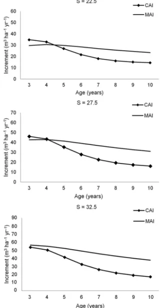
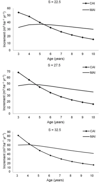
The estimations of the current annual increments and the mean annual increments in different site indexes are shown in Figures 4, 5, and 6.
Strategy A showed harvesting or thinning alterna-tives (where the MAI and CAI crossed each other) with approximately 4.6 years for the site index of 22.5 m and 4.2 years for the site index of 27.5 m (Figure 4). However, for the site index of 32.5 m, the curves of CAI and MAI did not intercept. Strategy B generated alternatives of harvesting or thinning approximately at 5.5 years for the site index of 2.5 m, 5.4 years for the site index of 27.5 m, and 5.0 years for the site index of 32.5 m. Strategy C, representing the Clutter models (Figure 6), generated alternatives at 5.1 years for the site index of 22.5 m, 4.9 years for the site index of 27.5 m, and 4.3 years for the site index of 32.5 m. Strategies A, B and C generated biologically consistent harvesting alternatives (i.e., higher rotations for less pro-ductive sites; Schumacher, 1939; Sevillano-Marco, 2009). This characteristic is very important to growth and yield Table 5 − Root mean square error [RMSE (%)] and relative bias
[Bias (%)] for the growth and yield equation strategies analyzed in volume of Eucalyptus camaldulensis × Eucalyptus urophylla
stands for the validation data.
Strategy
Site
General
22.5 27.5 32.5
RMSE Bias RMSE Bias RMSE Bias RMSE Bias % ---Strategy A 7.82 -0.90 8.22 2.28 5.37 -1.16 7.98 1.37 Strategy B 7.75 -0.19 8.01 1.95 5.81 -0.64 7.83 1.30 Strategy C 7.51 -4.84 9.05 2.48 5.82 -3.12 8.65 0.65 Where in: RMSE = root mean square error.
Figure 1 − Residual distribution (%) in function of the basal area estimated for Strategies A, B and C, respectively.
Figure 2 − Residual distribution (%) as a function of the volume estimated for the logistics model with covariates and the Clutter Model, respectively.
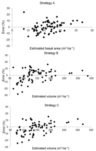
Figure 3 shows the residual distribution as a func-tion of the estimated volume for the projecfunc-tion growth and yield systems.
models because it constitutes a method for evaluating these models (Vanclay, 1994; Vanclay and Skovsgaard, 1997).
Conclusions
Models for projecting stand growth and yield, based on differential equations, can generate precise es-timations. The basal area projection models obtained by using differential equations were compatible with forest growth and yield. The logistics model with covariates was compatible with volume growth and yield. Strate-gies A and B generated different harvesting/thinning al-ternatives for different site indexes, presenting biological consistency. These equation systems are alternatives for projecting the growth and yield of forest plantations.
Acknowledgments
We thank the Coordination for the Improvement of Higher Level Personnel (CAPES) institute for the scholar-ship and the Minas Gerais State Foundation for Research Support (FAPEMIG) as a research project sponsor.
References
Bonet, J.A.; De-Miguel, S.; Martinez de Aragón, J.; Pukkala, T.; Palahí, M. 2012. Immediate effect of thinning on the yield of Lactarius group deliciosus in Pinus pinaster forests in Northeastern Spain. Forest Ecology and Management 265: 211-217.
Burkhart, H.E. 1971. Slash pine plantation yield estimates based on diameter distributions: an evaluation. Forest Science 17: 452-453. Clutter, J.L. 1963. Compatible growth and yield models for
loblolly pine. Forest Science 9: 355-371.
Davis, L.S.; Johnson, K.N.; Bettinger, P.; Howard, T. 2000. Forest Management. 4ed. McGraw-Hill, New York, NY, USA. Garcia, O. 1980. Modelling stand development with stochastic
differential equations. Biometrics 1: 63-68.
Garcia, O. 2005. Unifying sigmoid univariate growth equations. Forest Biometry, Modelling and Information Sciences 39: 1059-1072. Figure 3 − Residual distribution (%) as a function of the volume
estimated for the Strategies A, B and C, respectively.
Guimarães, M.A.M.; Calegario, N.; Carvalho, L.M.T.; Trugilho, P.F. 2009. Height-diameter models in forestry with inclusion of covariates. Cerne 15: 313-321.
Koya, P.R.; Goshu, A.T. 2013. Generalized mathematical model for biological growths. Open Journal of Modelling and Simulation 2: 42-54.
Kvalseth, T.O. 1985. Cautionary note about R². The American Statistician 39: 279-285.
Pienaar, L.V. 1979. An approximation of basal area growth after thinning based on growth in unthinned plantations. Forest Science 25: 223-232.
Pienaar, L.V.; Turnbull, K.J. 1973. The Chapman-Richards generalization of Von Bertalanffy’s growth model for basal area growth and yield in even-aged stands. Forest Science 19: 2-22. Ratkowsky, D.A. 1990. Handbook of Nonlinear Regression
Models. Marcel Dekker, New York, NY, USA.
Schumacher, X.A. 1939. A new growth curve and its application to timber yield. Journal of Forestry 37: 817-820.
Sevillano-Marco, E.; Fernández-Manso, A.; Castedo-Dorado, F. 2009. Development and applications of a growth model for Pinus radiata D. Don plantations in El Bierzo (Spain). Investigación Agraria: Sistemas y Recursos Forestales 18: 64-80.
Sullivan, A.D.; Clutter, J.L. 1972. A simultaneous growth and yield model for loblolly pine. Forest Science 18: 76-86.
Vanclay, J.K. 1994. Modelling Forest Growth and Yield: Applications to Mixed Tropical Forests. CAB International, Wallingford, UK.
Vanclay, J.K.; Skovsgaard, J.P. 1997. Evaluating forest growth models. Ecological Modelling 98: 1-12.
Wraith, J.M.; Or, D. 1998. Nonlinear parameter estimation using spreadsheet software. Journal of Natural Resources Life Sciences Education 27: 13-19.
Zeide, B. 1993. Analysis of growth equations. Forest Science 39: 594-616.
Zeide, B. 2004. Intrinsic units in growth modeling. Ecological Modelling 175: 249-259.
Figure 5 − Relationship between current annual increment (CAI) and mean annual increment (MAI) for Strategy B.