Block-based and structure-based techniques for
large-scale graph processing and visualization
Hugo Armando Gualdron Colmenares
Block-based and structure-based techniques for
large-scale graph processing and visualization
Master disssertation submitted to the Instituto de Ciências Matemáticas e de Computação – ICMC-USP, in partial fulfillment of the requirements for the degree of the Master Program in Computer Science and Computational Mathematics. FINAL VERSION
Concentration Area: Computer Science and Computational Mathematics
Advisor: Prof. Dr. José Fernando Rodrigues Júnior
USP – São Carlos January 2016
SERVIÇO DE PÓS-GRADUAÇÃO DO ICMC-USP Data de Depósito:
Ficha catalográfica elaborada pela Biblioteca Prof. Achille Bassi e Seção Técnica de Informática, ICMC/USP,
com os dados fornecidos pelo(a) autor(a)
Colmenares, Hugo Armando Gualdron
CGualdb Block-based and structure-based techniques for large-scale graph processing and visualization / Hugo Armando Gualdron Colmenares; orientador José Fernando Rodrigues Júnior. – São Carlos – SP, 2016.
80 p.
Dissertação (Mestrado - Programa de Pós-Graduação em Ciências de Computação e Matemática Computacional) – Instituto de Ciências Matemáticas e de Computação,
Universidade de São Paulo, 2016.
Hugo Armando Gualdron Colmenares
Tecnicas baseadas em bloco e em estrutura para
o processamento e visualização de grafos em
larga escala
Dissertação apresentada ao Instituto de Ciências Matemáticas e de Computação – ICMC-USP, como parte dos requisitos para obtenção do título de Mestre em Ciências – Ciências de Computação e Matemática Computacional. VERSÃO REVISADA
Área de Concentração: Ciências de Computação e Matemática Computacional
Orientador: Prof. Dr. José Fernando Rodrigues Júnior
For my wife Diana and my child Santiago,
Perseverance is stronger than fear.
ACKNOWLEDGEMENTS
I would like to express my sincere gratitude to my advisor Dr. José Fernado Rodrigues Júnior for his patience, motivation, and immense knowledge. His guidance helped me in all the time of research. My sincere thanks also goes to professor Dr. Duen Horng Chau for his research support during my internship at Georgia Tech University. I would also like to thank FAPESP for financially supporting my research. I thank my fellow labmates in for the inspiring discussions.
RESUMO
GUALDRON, H.. Block-based and structure-based techniques for large-scale graph pro-cessing and visualization. 2016. 80 f. Master dissertation (Master student Program in Computer Science and Computational Mathematics) – Instituto de Ciências Matemáticas e de Computação (ICMC/USP), São Carlos – SP.
Técnicas de análise de dados podem ser úteis em processos de tomada de decisão, quando padrões de interesse indicam tendências em domínios específicos. Tais tendências podem auxiliar a avaliação, a definição de alternativas ou a predição de eventos. Atualmente, os conjuntos de dados têm aumentado em tamanho e complexidade, impondo desafios para recursos modernos de hardware. No caso de grandes conjuntos de dados que podem ser representados como grafos, aspectos de visualização e processamento escalável têm despertado interesse. Arcabouços distribuídos são comumente usados para lidar com esses dados, mas a implantação e o gerenciamento de clusters computacionais podem ser complexos, exigindo recursos técnicos e financeiros que podem ser proibitivos em vários cenários. Portanto é desejável conceber técnicas eficazes para o processamento e visualização de grafos em larga escala que otimizam recursos de hardware em um único nó computacional. Desse modo, este trabalho apresenta uma técnica de visualização chamadaStructMatrixpara identificar relacionamentos estruturais em grafos reais. Adicionalmente, foi proposta uma estratégia de processamento bimodal em blocos, denominada
Bimodal Block Processing(BBP), que minimiza o custo de I/O para melhorar o desempenho do processamento. Essa estratégia foi incorporada a um arcabouço de processamento de grafos denominado M-Flashe desenvolvido durante a realização deste trabalho.Foram conduzidos experimentos a fim de avaliar as técnicas propostas. Os resultados mostraram que a técnica de visualização StructMatrix permitiu uma exploração eficiente e interativa de grandes grafos. Além disso, a avaliação do arcabouço M-Flash apresentou ganhos significativos sobre todas as abordagens baseadas em memória secundária do estado da arte. Ambas as contribuições foram validadas em eventos de revisão por pares, demonstrando o potencial analítico deste trabalho em domínios associados a grafos em larga escala.
ABSTRACT
GUALDRON, H.. Block-based and structure-based techniques for large-scale graph pro-cessing and visualization. 2016. 80 f. Master dissertation (Master student Program in Computer Science and Computational Mathematics) – Instituto de Ciências Matemáticas e de Computação (ICMC/USP), São Carlos – SP.
Data analysis techniques can be useful in decision-making processes, when patterns of interest can indicate trends in specific domains. Such trends might support evaluation, definition of alternatives, or prediction of events. Currently, datasets have increased in size and complexity, posing challenges to modern hardware resources. In the case of large datasets that can be represented as graphs, issues of visualization and scalable processing are of current concern. Distributed frameworks are commonly used to deal with this data, but the deployment and the management of computational clusters can be complex, demanding technical and financial resources that can be prohibitive in several scenarios. Therefore, it is desirable to design efficient techniques for processing and visualization of large scale graphs that optimize hardware resources in a single computational node. In this course of action, we developed a visualization technique namedStructMatrixto find interesting insights on real-life graphs. In addition, we proposed a graph processing frameworkM-Flashthat used a novel, bimodal block processing strategy (BBP) to boost computation speed by minimizing I/O cost. Our results show that our visualization technique allows an efficient and interactive exploration of big graphs and our framework M-Flash significantly outperformed all state-of-the-art approaches based on secondary memory. Our contributions have been validated in peer-review events demonstrating the potential of our finding in fostering the analytical possibilities related to large-graph data domains.
LIST OF FIGURES
Figure 1 – The vocabulary of graph structures considered in our methodology. From (a) to (g), illustrative examples of the patterns that we consider; we process variations on the number of nodes and edges of such patterns. . . 30 Figure 2 – Adjacency Matrix layout. . . 34 Figure 3 – StructMatrix in the WWW-barabasi graph with colors displaying the sum of
the sizes of two connected structures; in the graph, stars refer to websites with links to other websites. . . 35 Figure 4 – StructMatrix in the Wikipedia-vote graph with values displaying the sum of
the sizes of two connected structures; in this graph, stars refer to users who got/gave votes from/to other users. . . 35 Figure 5 – Scalability of theStructMatrixand VoG techniques; although VoG is
near-linear to the graph edges, StructMatrix overcomes VoG for all the graph sizes. . . 37 Figure 6 – DBLP Zooming on thefullclique section. . . 39 Figure 7 – StructMatrix with colors in log scale indicating the size of the structures
interconnected in the road networks of Pennsylvania (PA), California (CA) and Texas(TX). Again, stars appear as the major structure type; in this case they correspond to cities or to major intersections. . . 39 Figure 8 – Organization of edges and vertices in M-Flash. Left (edges): example of a
graph’s adjacency matrix (in light blue color) organized in M-Flash using 3 logical intervals (β =3); G(p,q) is an edge block with source vertices in interval I(p) and destination vertices in interval I(q); SP(p) is a source-partitioncontaning all blocks with source vertices in intervalI(p);DP(q)is a
destination-partitioncontaning all blocks with destination vertices in interval
I(q). Right (vertices): the data of the vertices askvectors (γ1 ... γk), each
one divided intoβ logical segments. . . 46 Figure 9 – M-Flash’s computation schedule for a graph with 3 intervals. Vertex intervals
Figure 10 – Example I/O operations to process thedenseblockG(2,1). . . 48 Figure 11 – Example I/O operations for step 1 ofsource-partitionSP3. Edges of SP1are
combined with their source vertex values. Next, the edges are divided by
β destination-partitionsin memory; and finally, edges are written to disk. On Step 2 ,destination-partitionsare processed sequentially. Example I/O operations for step 2 ofdestination-partitionDP(1). . . 49 Figure 12 – Runtime of PageRank for LiveJournal, Twitter and YahooWeb graphs with
8GB of RAM. M-Flash is 3X faster than GraphChi and TurboGraph. (a & b): for smaller graphs, such as Twitter, M-Flash is as fast as some exist-ing approaches (e.g., MMap) and significantly faster than other (e.g., 4X of X-Stream). (c): M-Flash is significantly faster than all state-of-the-art approaches for YahooWeb: 3X of GraphChi and TurboGraph, 2.5X of X-Stream, 2.2X of MMap. . . 57 Figure 13 – Runtimes of the Weakly Connected Component problem for LiveJournal,
Twitter, and YahooWeb graphs with 8GB of RAM. (a & b): for the small (LiveJournal) and medium (Twitter) graphs, M-Flash is faster than, or as fast as, all the other approaches. (c) M-Flash is pronouncedly faster than all the state-of-the-art approaches for the large graph (YahooWeb): 9.2X of GraphChi and 5.8X of X-Stream. . . 58 Figure 14 – Runtime comparison for PageRank (1 iteration) over the YahooWeb graph.
M-Flash is significantly faster than all the state-of-the-art for three different memory settings, 4 GB, 8 GB, and 16 GB. . . 60 Figure 15 – I/O operations for 1 iteration of PageRank over the YahooWeb graph.
M-Flash performs significantly fewer reads and writes (in green) than other approaches. M-Flash achieves and sustains high-speed reading from disk (the “plateau” in top-right), while other methods do not. . . 60 Figure 16 – I/O cost usingDBP,SPP, andBBPfor LiveJournal, Twitter and YahooWeb
Graphs using different memory sizes. BBPmodel always performs fewer I/O operations on disk for all memory configurations. . . 62 Figure 17 – I/O cost using DBP, SPP, and BBP for a graph with densitiesk={3,5,10,30}.
Graph density is the average vertex degree, |E| ≈ k|V|. DBP increases considerably I/O cost when RAM is reduced,SPPhas a constant I/O cost andBBPchooses the best configuration considering the graph density and available RAM. . . 63 Figure 18 – This results were published in our paper [1]. . . 67 Figure 19 – AUC visualization of the data generated for a co-authoring snapshot of DBLP
Figure 20 – Plot of metric SP′Importance. (a) Raw curve of Equation 4.1. (b) Count-ing (3D histogram) of authors in relation to the possible values of metric
LIST OF ALGORITHMS
Algoritmo 1 – StructMatrix algorithm . . . 32
Algoritmo 2 – Structure classification . . . 32
Algoritmo 3 – MAlgorithm: Algorithm Interface for coding in M-Flash . . . 51
Algoritmo 4 – PageRank in M-Flash . . . 51
Algoritmo 5 – Weak Connected Component in M-Flash . . . 52
Algoritmo 6 – SpMV for weighted graphs in M-Flash . . . 52
Algoritmo 7 – Lanczos Selective Orthogonalization . . . 53
LIST OF TABLES
Table 1 – Description of the major symbols used in this work. . . 31
Table 3 – Structures found in the datasets considering a minimum size of 5 nodes. . . . 36
Table 2 – Description of the graphs used in our experiments. . . 36
Table 4 – Real graph datasets used in our experiments. . . 55
Table 5 – Preprocessing time (seconds) . . . 56
CONTENTS
1 INTRODUCTION . . . 23
1.1 Motivation . . . 23
1.2 Problem . . . 23
1.3 Hypotheses . . . 24
1.4 Rationale . . . 24
1.5 Contributions . . . 25
2 MILLION-SCALE VISUALIZATION OF GRAPHS BY MEANS OF
STRUCTURE DETECTION AND DENSE MATRICES . . . 27
2.1 Initial considerations . . . 27
2.2 Introduction . . . 27
2.3 Related works . . . 28
2.3.1 Large graph visualization . . . 28 2.3.2 Structure detection . . . 29
2.4 Proposed method: StructMatrix . . . 30
2.4.1 Overview of the graph condensation approach . . . 30 2.4.2 StructMatrix algorithm . . . 32 2.4.3 Adjacency Matrix Layout . . . 33
2.5 Experiments . . . 36
2.5.1 Graph condensations . . . 36 2.5.2 Scalability . . . 36 2.5.3 WWW and Wikipedia . . . 37 2.5.4 Road networks . . . 38 2.5.5 DBLP . . . 40
2.6 Conclusions . . . 40
2.7 Final considerations . . . 41
3 M-FLASH: FAST BILLION-SCALE GRAPH COMPUTATION
US-ING A BIMODAL BLOCK PROCESSUS-ING MODEL . . . 43
3.1 Initial considerations . . . 43
3.2 Introduction . . . 43
3.3 Related work . . . 45
3.4.1 Graphs Representation in M-Flash . . . 46 3.4.2 The M-Flash Processing Model . . . 47 3.4.3 Programming Model in M-Flash . . . 51 3.4.4 System Design & Implementation . . . 52
3.5 Evaluation . . . 54
3.5.1 Graph Datasets . . . 55 3.5.2 Experimental Setup . . . 55 3.5.3 PageRank . . . 56 3.5.4 Weakly Connected Component . . . 57 3.5.5 Spectral Analysis using The Lanczos Algorithm . . . 58 3.5.6 Effect of Memory Size . . . 59 3.5.7 Input/Output (I/O) Operations Analysis . . . 59 3.5.8 Theoretical (I/O) Analysis . . . 60
3.6 Conclusions . . . 62
3.7 Final considerations . . . 63
4 FURTHER RESULTS . . . 65
4.1 Initial considerations . . . 65
4.2 Multimodal analysis of DBLP . . . 65
4.3 Final considerations . . . 68
5 CONCLUSIONS . . . 71
23
CHAPTER
1
INTRODUCTION
1.1
Motivation
The computational technology in the XXI century has provided powerful resources to generate digital content, massive access to information, and connectivity between systems, people and electronic devices. This technology produces data in unprecedented scale, having received different denominations: big data, web scale, massive data, planetary or large scale 1. It is not easy to measure the size of the digital information currently being produced, but some works suggest its size and growth. The Twitter company, for instance, publicly demonstrated the evolution of its social network in 2011 [3]; according to which the time between the first and the billion-th message was of only three years. Recently, a work of Gudinava et al.[4] estimates that just a small share of 1 petabyte of the data currently produced is public; and that only 22 percent of this data can be considered useful. This data contains intrinsic and valuable information, and companies likeGeneral ElectricandAccenturehave shown that data analysis techniques are a differential factor in industrial competitiveness [5].
1.2
Problem
A relevant set of the data produced in planetary scale describes relations that can be represented using graphs. Graph representations are useful to analyze and optimize problems in domains such as public politics, commercial decisions, security and social networks. Usual graph processing and visualization systems assume that the graph data fit entirely in the main memory; however, the current size of big graphs can be equivalent to a whole disk or even an array of disks with storage needs up to 100x larger than RAM. For instance, the Twitter graph [6] can be measured in terabyte units; the Yahoo Web graph [7] has more than 1 billion nodes and almost 7 billion edges; and the clickstreams graph [8] reaches petabyte magnitude. Such graphs are a challenge
24 Chapter 1. Introduction
for data analysis because they require powerful resources for processing, and complex models to achieve tasks with limited resources. This issue happens because graph algorithms usually are based on depth or on breadth processing techniques that are not parallelizable. Existing frameworks, based on vertex-centric [9] [10] and edge-centric [11] processing, tackle with those limitations; but they do not optimize resource utilization, failing in sub-optimal approaches for processing planetary-scale graphs.
1.3
Hypotheses
Considering optimization of resources as a cornerstone for processing planetary-scale graphs, and for interactive visualization as a desirable tool in decision-making, we explored two possibilities:
1. we researched on how to detect macro features of very large graphs, mining recurrent patterns like cliques, bi-partite cores, stars and chains; we also analyzed relevant graph domains, characterizing them according to the cardinality, distribution, and relationship of their patterns, leading to the following hypothesis:relations between recurrent and simple patterns characterize graph domains providing interesting insights through exploratory visualization;
2. we designed an algorithmic framework that minimizes disk and memory access during vertex-centric and edge-centric processing using only one computational node. We fo-cused on how to minimize I/O communication, taking advantage of hardware capabilities and advanced algorithm design. Accordingly, we worked on validating the following hypothesis:a framework focused on minimizing I/O communication is able to boost the processing speed of planetary-scale graphs that do not fit in RAM.
1.4
Rationale
Large graph visualization is a research area widely studied [12, 13, 14, 15, 16, 17, 18, 19, 20, 21, 22, 23]; however, there are not optimal solutions considering scalability and interaction for many visual tasks [24]. In this research area, visual analysis has two predominant paradigms:
1.5. Contributions 25
(both visual and computational) and interactivity in order to make sense of planetary-scale graphs, as delineated in our first hypothesis. We detail this work in Chapter 2 along with further literature review.
Graph visualization techniques usually require efficient algorithms for graph partitioning, summarization, filtering, clustering or some other task related to graph mining. The computation of such patterns properties, considering planetary-scale graphs, demands distributed and parallel frameworks. The work of Pregel [9], for example, defines a seminal framework that provides a simple programming interface based on message passing; it uses the paradigm “think like vertex” hiding the complexity of distributed systems. Another framework, named GBase [38], uses a MapReduce [39]/Hadoop[40] implementation for graph processing through a block compress partition scheme; in turn, GraphLab [10] introduces an asynchronous, dynamic and graph-parallel scheme for machine learning that permits implementations of many algorithms for graphs; and PowerGraph [41] improves the approach of GraphLab by exploiting power-law distributions – common in graphs of many domains. There are other distributed implementations as the Apache Giraph [42], Trinity [43] and GraphX [44]; but, in general, distributed approaches may not always be the best option, because they can be expensive to build [45] and hard to maintain and optimize.
In addition to the distributed frameworks, single-node processing solutions have recently reached a comparative performance to distributed systems for similar algorithms [46]. These frameworks use secondary memory as an extension of main memory (RAM). GraphChi [45] was one of the first single-node approaches to avoid random disk/edge accesses; it uses a vertex-centric model improving the performance for mechanical disks. Another solution, X-Stream [11] introduced an edge-centric model that achieved better performance over the vertex-centric approaches, it did so by favoring sequential disk access over unordered data. In another way, the FlashGraph framework [47] provides an efficient implementation that considers enough RAM memory for storing vertex values, but its scalability is limited. Among the existing works designed for single-node processing, some of them are restricted to SSDs. These works rely on the remarkable low-latency and improved I/O of SSDs compared to magnetic disks. This is the case of TurboGraph [48] and RASP [49], which rely on random accesses to the edges — not well supported over magnetic disks. In the current research, we have extensively studied these framework in order to design a new methodology that surpasses the performance of all of the previous single-node processing frameworks. In Chapter 3, we provide further details and results that demonstrate our second hypothesis.
1.5
Contributions
26 Chapter 1. Introduction
Firstly, we proposed a visualization technique concerning the principle that graphs can be characterized using simple structures, common in many graph domains. Instead of node relations, we represented the graph using an upper level of abstraction where sets of nodes and edges are associated with chains, stars, cliques and bipartite-cores. We designed an efficient algorithm that cuts power-law graphs iteratively. It removes hubs progressively to detect connected components in the graph; at once, it classifies each connected component in a simple structure when is possible and, when not, it applies the same cut process for each one. After detection of structures, as detailed in chapter 2, our algorithm visualizes the structures using a dense-matrix layout in which we can study the distribution of structures, their size, and how they are related.
27
CHAPTER
2
MILLION-SCALE VISUALIZATION OF
GRAPHS BY MEANS OF STRUCTURE
DETECTION AND DENSE MATRICES
2.1
Initial considerations
Large graph visualization has been a prolific research area for years, and new techniques for processing, interaction and visualization of big graphs are usually proposed to deal with sensemaking and scalability. Given a large-scale graph with millions of nodes and millions of edges, how to reveal macro patterns of interest, like cliques, bi-partite cores, stars, and chains? Furthermore, how to visualize such patterns altogether getting insights from the graph to support wise decision-making? Although there are many algorithmic and visual techniques to analyze graphs, none of the existing approaches are able to present the structural information of graphs at million scale; hence, in this chapter, we present our first contribution StructMatrix, a methodology aimed at high-scale visual inspection of graph structures with the goal of revealing macro patterns of interest.
2.2
Introduction
28 Chapter 2. Million-scale visualization of graphs by means of structure detection and dense matrices
characterizes the way a given graph is understood.
While some features of large graphs are detected by algorithms that produce hundreds of tabular data, these features can be better noticed with the aid of visual representations. In fact, some of these features, given their large cardinality, are intelligible, in a timely manner, exclusively with visualization. Considering this approach, we propose StructMatrix, a method-ology that combines a highly scalable algorithm for structure detection with a dense matrix visualization. With StructMatrix, we introduce the following contributions:
1. Methodology:we introduce innovative graph processing and visualization techniques to detect macro features of very large graphs;
2. Scalability:we show how to visually inspect graphs with magnitudes far bigger than those of previous works;
3. Analysis:we analyze relevant graph domains, characterizing them according to the cardi-nality, distribution, and relationship of their structures.
The rest of the paper presents related works in Section 3.3, the proposed methodology in Section 2.4, experimentation in Section 2.5, and conclusions in Section 2.6. Table 1 lists the symbols used in our notation.
2.3
Related works
2.3.1
Large graph visualization
There are many works about graph visualization, however, the vast majority of them is not suited for large-scale. Techniques that are based on node-link drawings cannot, at all, cope with the needs of just a few thousand edges that would not fit in the display space. Edge bundling [50] techniques are also limited since they do not scale to millions of nodes and also because they are able to present only the main connection pathways in the graph, disregarding potentially useful details. Other large-scale techniques are visual in a different sense; they present plots of calculated features of the graph instead of depicting their structural information. This is the case of Apolo [51], Pegasus [52], and OddBall [53]. There are also techniques [54] that rely on sampling to gain scalability, but this approach assumes that parts of the graph will be absent; parts that are of potential interest.
2.3. Related works 29
The main challenge of using clustering techniques is to find an aggregation algorithm that produces a hierarchy that is meaningful to the user. There are also matrix visualization layouts as MatLink [57] and NodeTrix [58] combining Node-Link and adjacency representations to increase readability and scalability, but those approaches are not enough to visualize large-scale graphs.
Net-Ray [30] is another technique working at large scale; it plots the original adjacency matrix of one large graph in the much smaller display space using a simple projection: the original matrix is scaled down by means of straight proportion. This approach causes many edges to be mapped to one same pixel; this is used to generate a heat map that informs the user of how many edges are in a certain position of the dense matrix.
In this work, we extend the approach of adjacency matrices, as proposed by Net-Ray, improving its scalability and also its ability to represent data. In our methodology, we introduce two main improvements: (1) our adjacency matrix is not based on the classic node-to-node representation; we first condense the graph as a collection of smaller structures, defining a structure-to-structure representation that enhances scalability as more information is represented and less compression of the adjacency matrix is necessary; and (2) our projection is not a static image but rather an interactive plotting from which different resolutions can be extracted, including the adjacency matrix with no overlapping – of course, considering only parts of the matrix that fit in the display.
2.3.2
Structure detection
The principle of StructMatrix is that graphs are made of simple structures that appear recurrently in any graph domain. These structures include cliques, bipartite cores, stars, and chains that we want to identify. Therefore, a given network can be represented in an upper level of abstraction; instead of nodes, we use sets of nodes and edges that correspond to substructures. The motivation here is that analysts cannot grasp intelligible meaning out of huge network structures; meanwhile, a few simple substructures are easily understood and often meaningful. Moreover, analyzing the distribution of substructures, instead of the distribution of single nodes, might reveal macro aspects of a given network.
Partitioning (shattering) algorithms
StructMatrix, hence, depends on a partitioning (shattering) algorithm to work. Many algorithms can solve this problem, like Cross-associations [59], Eigenspokes [60], and METIS [61], and VoG [62]. We verified that VoG overcomes the others in detecting simple recurrent structures considering a limited well-known set.
30 Chapter 2. Million-scale visualization of graphs by means of structure detection and dense matrices
Figure 1 – The vocabulary of graph structures considered in our methodology. From (a) to (g), illustrative examples of the patterns that we consider; we process variations on the number of nodes and edges of such patterns.
lattices, the degree distribution of real-world networks obeys to power laws; in such graphs, a few nodes have a very high degree, while the majority of the nodes have low degree. Kang and Faloutsos also demonstrated that large networks are easily shattered by an ordered “removal” of the hub nodes. In fact, after each removal, a small set of disconnected components (satellites) appear, while the majority of the nodes still belong to the giant connected component. That is, the disconnected components were connected to the network only by the hub that was removed and, by progressively removing the hubs, the entire graph is scanned part by part. Interestingly, the small components that appear determine a partitioning of the network that is more coherent than cut-based approaches [64]. The technique works for any power-law graph without domain-specific knowledge or specific ordering of the nodes.
For the sake of completeness and performance, we designed a new algorithm that, following the Slash-Burn technique, extends algorithm Vog with parallelism, optimizations, and an extended vocabulary of structures, as detailed in Section 2.4.2. Our results demonstrated better performance while considering a larger set of structures.
2.4
Proposed method: StructMatrix
As we mentioned before,StructMatrixdraws an adjacency matrix in which each line/column is a structure, not a single node; besides that, it uses a projection-based technique to “squeeze” the edges of the graph in the available display space, together with a heat mapping to inform the user of how big are the structures of the graph. In the following, we formally present the technique.
2.4.1
Overview of the graph condensation approach
2.4. Proposed method: StructMatrix 31
Notation Description
G(V,E) graph with V vertices and E edges
S,Sx structure-set n,|S| cardinality ofS M,mx,y StructMatrix
f c,nc full and near clique resp.
f b,nb full and near bipartite core resp.
st, f s,ch star, false star and chain resp.
ψ vocabulary (set) of structures
D(si,sj) Number of edges between
structure instancessiandsj
Table 1 – Description of the major symbols used in this work.
Falsestars are structures similar to stars (a central node surrounded by satellites), but whose satellites have edges to other nodes, indicating that the star may be only a substructure of a bigger structure – see Figure 1. A near-clique or ε-near clique is a structure with 1−ε
(0<ε<1) percent of the edges that a similar full clique would have; the same holds for near bipartite cores. In our case, we are considering ε=0.2 so that a structure is considered near cliqueornearbipartite core, if it has at least 80 percent of the edges of the corresponding full structure.
The rationale behind the set of structuresψ is that (a) cliques correspond to strongly connected sets of individuals in which everyone is related to everyone else; cliques indicate communities, closed groups, or mutual-collaboration societies, for instance. (b) Chains corre-spond to sequences of phenomena/events like those of “spread the word”, according to which one individual passes his experience/feeling/impression/contact with someone else, and so on, and so forth; chains indicate special paths, viral behavior, or hierarchical processes. (c) Bipartite cores correspond to sets of individuals with specific features, but with complementary interac-tion; bipartite cores indicate the relationship between professors and students, customers and products, clients and servers, to name a few. And, (d) stars correspond to special individuals highly connected to many others; stars indicate hub behavior, authoritative sites, intersecting paths, and many other patterns.
32 Chapter 2. Million-scale visualization of graphs by means of structure detection and dense matrices
2.4.2
StructMatrix algorithm
As mentioned earlier, our algorithm is based on a high-degree ordered removal of hub nodes from the graph; the goal is to accomplish an efficient shattering of the graph, as introduced in Section 2.3.2. As we describe in Algorithm 1, our process relies on a queue, Φ, which contains the unprocessed connected components (initially the whole graph), and a setΓthat contains the discovered structures. In line 4, we explore the fact that the problem is straight parallelizable by triggering threads that will process each connected component in queueΦ. In the process, we proceed with the ordered removal of hubs – see line 5, which produces a new set of connected components. With each connected component, we proceed by detecting a structure instance in line 7, or else, pushing it for processing in line 10. The detection of structures and the identification of their respective types occur according to Algorithm 2, which uses edge arithmetic to characterize each kind of structure.
Algorithm 1StructMatrix algorithm
Require: GraphG= (E,V)
Ensure: ArrayΓcontaining the structures found inG
1: Let be queueΦ={G}and setΓ={} 2: whileΦis not emptydo
3: H=Pop(Φ) /*Extract the first item from queueΦ*/
4: SUBFUNCTION Thread(H) BEGIN /*In parallel*/
5: H′=“H without the 1% nodes with highest degree”
6: foreach connected componentcc∈H′do
7: ifcc∈ψ using Algorithm 2 then
8: Add(Γ, cc)
9: else
10: Push(Φ, cc)
11: end if
12: end for
13: END Thread(H)
14: end while
Algorithm 2Structure classification
Require: SubgraphH= (E,V);n=|V|andm=|E|
1: ifm = n(n2−1) then returnfc
2: else ifm>(1−ε)∗n(n2−1) then returnnc
3: else ifm< n2
4 andH= (E,Va∪Vb)is bipartitethen
4: ifm=|Va| ∗ |Vb|then returnfb
5: else ifm>(1−ε)∗ |Va| ∗ |Vb|then returnnb
6: else if|Va|=1 or|Vb|=1then returnst
7: else ifm=n−1then returnch
8: end if
9: end ifreturnundefined structure
2.4. Proposed method: StructMatrix 33
of structures rather than favoring optimum compression; it uses parallelism for improved per-formance; and considers a larger set of structures. In Section 2.5, we demonstrate these aspects through experimentation.
2.4.3
Adjacency Matrix Layout
A graphG=hV,EiwithV vertices andE edges can be expressed as a set of structural instances
S={s0,s2, . . . ,s|S|−1}, wheresiis a subgraph ofGthat is categorized – see Figure 1 and Table 1
– according to the functiontype(s):S→ψ. To create the adjacency matrix of structures, first we identify the setSof structures in the graph and categorize each one. Following, we definen=|S|
to refer to the cardinality ofS.
As depicted in Figure 2, each type of structure defines a partition in the matrix, both horizontally and vertically, determining subregions in the visualization matrix. In this matrix, a given structure instance corresponds to a horizontal and to a vertical line (w.r.t. the subregions) in which each pixel represents the presence of edges (one or more) between this structure and the others in the matrix. Therefore, the matrix is symmetric and supports the representation of relationships (edges) between all kinds of structure types. Formally, the elementsmi,jof a
StructMatrixMn×n, 0<i<(n−1)and 0< j<(n−1)are given by:
mi,j=
(
1, i f D(si,sj)>0;
0otherwise. (2.1)
whereD:S×S→Nis a function that returns the number of edges between two given structure
instances. For quick reference, please refer to Table 1.
In this work, we focus on large-scale graphs whose corresponding adjacency matrices do not fit in the display. This problem is lessened when we plot the structures-structures matrix, instead of the nodes-nodes matrix. However, due to the magnitude of the graphs, the problem persists. We treat this issue with a density-based visualization for each subregion formed by two types of structures(ψi,ψj),ψi∈ψ andψj∈ψ – for example,(f s,f s),(f s,st), ..., and so on. In
each subregion, we map each point of the original matrix according to a straight proportion. We map the lower, left boundary point(xmin,ymin)to the center of the lower, left boundary pixel;
and the upper, right boundary point(xmax,ymax)to the center of the upper, right boundary pixel.
The remaining points are mapped as(x,y)→(ρx,ρy)for:
ρx=R(ψi,ψj) +
l
(Resx−1)xmax−x−xminxmin+12
m
ρy=R(ψi,ψj) +
l
(Rexy−1)ymaxy−−yminymin+12
m
(2.2)
34 Chapter 2. Million-scale visualization of graphs by means of structure detection and dense matrices
Figure 2 – Adjacency Matrix layout.
presented, these parameters allow for interactive grasping of details.
Each set of edges connecting two given structures is then mapped to the respective subregion of the visualization where the structures’ types cross. Inside each structure subregion we add an extra information by ordering the structure instances according to the number of edges that they have to other structures; that is, by|
S|−1
∑
i=0
D(s,si).
Therefore, the structures with the largest number of edges to other structures appear first – more at the bottom left, less at the top right, of each subregion as explained in Figure 2.
In the visualization, each horizontal/vertical line (w.r.t. the subregions) corresponds to a few hundred or thousand structure instances; and each pixel corresponds to a few hundred or thousand edges. We deal with that by not plotting the matrix as a static image, but as a dynamic plot that adapts to the available space; hence, it is possible to select specific areas of the matrix and see more details of the edges. It is possible to regain details until reaching parts the original plot, when all the edges are visible.
2.4. Proposed method: StructMatrix 35
(a)Normal scale. (b)Log scale.
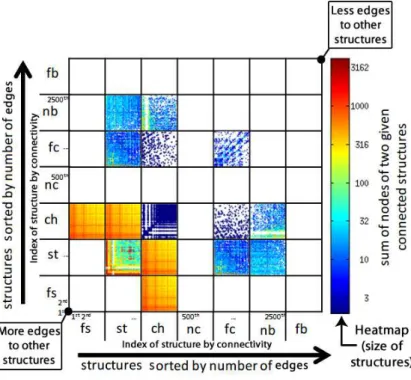
Figure 3 – StructMatrix in the WWW-barabasi graph with colors displaying the sum of the sizes of two connected structures; in the graph, stars refer to websites with links to other websites.
(c)Normal scale. (d)Log scale.
Figure 4 – StructMatrix in the Wikipedia-vote graph with values displaying the sum of the sizes of two connected structures; in this graph, stars refer to users who got/gave votes from/to other users.
of a StructMatrixMn×n, 0<i<(n−1)and 0< j<(n−1)are given by:
mi,j=
C(NNodes(si) +NNodes(sj)),
i f D(si,sj)>0;
0otherwise.
(2.3)
whereNNodes:S→Nis a function that returns the number of nodes of a given structure
instance; andC:N→[0.0,1.0]is a function that returns a continuous value between 0.0 (cool
36 Chapter 2. Million-scale visualization of graphs by means of structure detection and dense matrices
Graph fs st ch nc fc nb fb
DBLP 122,983 (76%) 7,585(5%) 3,096(2%) 2,656(2%) 24,551(15%) 14(<1%)
-WWW-barabasi 4,957(32%) 8,146(52%) 851(5%) 541(3%) 283(2%) 556(4%) 318(2%)
cit-HepPh 11,449(79%) 1,948(13%) 840(6%) 120(1%) 44 (4<1%) 35(<1%) 43(<1%)
Wikipedia-vote 1,112(65%) 564(33%) 29 (2%) - - 1(<1%)
-Epinions 4,518(52%) 2,725(31%) 1,247(14%) 28 (%) 21(%) 150(2%) 3(<1%)
Roadnet PA 11,825(23%) 22,934(45%) 13,748(27%) - - 2,668(5%)
-Roadnet CA 24,193(27%) 34,781(39%) 26,236(29%) - - 3,763(4%)
-Roadnet TX 15,595(25%) 27,094(43%) 17,457(28%) - - 2,468(4%)
-Table 3 – Structures found in the datasets considering a minimum size of 5 nodes.
2.5
Experiments
Table 2 describes the graphs we use in the experiments.
Name Nodes Edges Description
DBLP 1,366,099 5,716,654 Collaboration network Roads of PA 1,088,092 1,541,898 Road net of Pennsylvania
Roads of CA 1,965,206 2,766,607 Road net of California Roads of TX 1,379,917 1,921,660 Road net of Texas
WWW-barabasi 325,729 1,090,108 WWW in nd.edu Epinions 75,879 405,740 Who-trusts-whom network
cit-HepPh 34,546 420,877 Co-citation network
Wiki-vote 7,115 100,762 Wikipedia votes
Table 2 – Description of the graphs used in our experiments.
2.5.1
Graph condensations
Table 3 shows the condensation results of the structure detection algorithm over each dataset, already considering the extended vocabulary and structures with minimum size of 5 nodes – less than 5 nodes could prevent to tell apart the structure types. The columns of the table indicate the percentage of each structure identified by the algorithm. For all the datasets, the false star was the most common structure; the second most common structure was the star, and then the chain, especially observed in the road networks. The improvement of the visual scalability of
StructMatrix, compared to former work Net-Ray, is as big as the amount of information that is “saved” when a graph is modeled as a structure-to-structure adjacency matrix, instead of a node-to-node matrix.
2.5.2
Scalability
2.5. Experiments 37
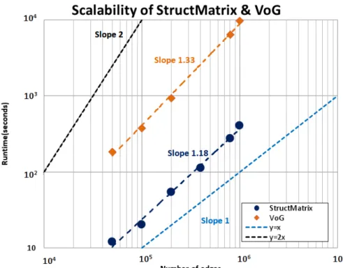
Figure 5 – Scalability of theStructMatrixand VoG techniques; although VoG is near-linear to the graph edges, StructMatrix overcomes VoG for all the graph sizes.
VoG are near-linear on the number of edges of the input graph, however StructMatrix overcomes VoG for all the graph sizes.
2.5.3
WWW and Wikipedia
In Figures 3 and 4, one can see the results of StructMatrix for graphs WWW-barabasi (325,729 nodes and 1,090,108 edges) and Wikipedia-vote (7,115 nodes and 100,762 edges) condensed as described in Table 3. For graph WWW-barabasi, Figure 3a shows the StructMatrix with linear color encoding, and Figure 3b shows the StructMatrix with logarithmic color encoding. For the Wikipedia-vote graph, the same visualizations are presented in Figures 3c and 3d. We observe the following factors in the visualizations:
• the share of structures: WWW-barabasi presents a clear majority of stars, followed by false stars, and chains, while the Wikipedia-vote presents a majority of false stars, followed by stars, and chains; in both cases, stars strongly characterize each domain, as expected in websites and in elections;
• the presence of outliers in WWW-barabasi, spotted in red; and the presence of structures globally and strongly connected in Wikipedia-vote, depicted as reddish lines across the visualization;
38 Chapter 2. Million-scale visualization of graphs by means of structure detection and dense matrices
• the effect of the logarithmic color scale; its use results in a clearer discrimination of the magnitudes of the color-mapped values, what helps to perceive the distribution of the values; more skewed in WWW and more uniform in Wikipedia.
The stars and false stars of the WWW graph in Figure 3b refer to sites with multiple pages and many out-links – bigger sites are reddish, more connected sites to the left. The visualization is able to indicate the big stars (sites) that are well-connected to other sites (reddish lines), and also the big sites that demand more connectivity – reddish isolated pixels. The chains indicate site-to-site paths of possibly related semantics, an occurrence not so rare for the WWW domain. There is also a set of reasonably small, interconnected sites that connect only with each other and not with the others – these sites determine blank lines in the visualization and their sizes are noticeable in dark blue at the bottom-left corner of the star-to-star subregion. Such sites should be considered as outliers because, although strongly connected, they limit their connectivity to a specific set of sites.
While the Wikipedia graph is mainly composed of stars, just like the WWW graph, the Wikipedia graph is quite different. Its structures are more interconnected defining a highly populated matrix. That means that users (contributors) who got many votes to be elected as administrators in Wikipedia, also voted in many other users. The sizes of the structures, indicated by color, reveal the most voted users, positioned at the bottom-left corner – the color pretty much corresponds to the results of the elections: of the 2,794 users, only 1,235 users had enough votes to be elected administrators (nearly 50% of the reddish area of the matrix). There are also a few chains, most of them connected to stars (users), especially the most voted ones – it becomes evident that the most voted users also voted on the most voted users. This is possibly because, in Wikipedia, the most active contributors are aware of each other.
2.5.4
Road networks
On the road networks, if we consider the stars segment (“st”), each structure corresponds to a city (the intersecting center of the star); therefore, the horizontal/vertical lines of pixels correspond to the more important cities that act as hubs in the road system. ItsStructMatrixvisualization – Figure 7 – showed an interesting pattern for all the three road datasets: in the figure, one can see that the relationships between the road structures is more probable in structures with similar connectivity. This fact is observable in the curves (diagonal lines of pixels) that occur in the visualization – remember that the structures are first ordered by type into segments, and then by their connectivity (more connected first) in each segment.
2.5. Experiments 39
(a)All types of structures. (b)Only thefc-fcsub region with details.
Figure 6 – DBLP Zooming on thefullclique section.
Figure 7 – StructMatrix with colors in log scale indicating the size of the structures interconnected in the road networks of Pennsylvania (PA), California (CA) and Texas(TX). Again, stars appear as the major structure type; in this case they correspond to cities or to major intersections.
1. cities that connect to most of the other cities acting as interconnecting centers in the road structure; these cities are of different importance and occur in small number – around 6 for each state that we studied;
2. there is a hierarchical structure dictated by the connectivity (importance) of the cities; in this hierarchy, the connections tend to occur between cities with similar connectivity; one consequence of this fact is that going from one city to some other city may require one to first “ascend” to a more connected city; actually, for this domain, the lines of pixels in the visualization correspond to paths between cities, passing through other cities – the bigger the inclination of the line, the shorter the path (the diagonal is the longest path);
40 Chapter 2. Million-scale visualization of graphs by means of structure detection and dense matrices
From these visualizations and patterns, we notice that the StructMatrix visualization is a quick way (seconds) to represent the structure of graphs on the order of million-nodes (intersections) and million-edges (roads). For the specific domain of roads, the visualization spots the more important cities, the hierarchy structure, outlier roads that should be inspected closer, and even, the adequacy of the roads’ inter connectivity. This last issue, for example, may indicate where there should be more roads so as to reduce the pathway between cities.
2.5.5
DBLP
In theStructMatrixof the DBLP co-authoring graph – see Figure 6a – it is possible to see a huge number of false stars. This fact reflects the nature of DBLP, in which works are done by advisors who orient multiple students along time; these students in turn connect to other students defining new stars and so on. A minority of authors, as seen in the matrix, concerns authors whose students do not interact with other students defining stars properly said. The presence of full cliques (fc) is of great interest; sets of authors that have co-authorship with every other author. Full cliques are expected in the specific domain of DBLP because every paper defines a full clique among its authors – this is not true for all clique structures, but for most of them.
In Figure 6b, we can see the full clique-to-full clique region in more details and with some highlights indicated by arrows. The Figure highlights some notorious cliques:k1refers to
the publication with title “A 130.7mm 2-layer 32Gb ReRAM memory device in 24nm technology" with 47 authors; k2 refers to paper “PRE-EARTHQUAKES, an FP7 project for integrating observations and knowledge on earthquake precursors: Preliminary results and strategy" with 45 authors; andk3refers to paper “The Biomolecular Interaction Network Database and related tools 2005 update" with 75 authors. These specific structures were noticed due to their colors, which indicate large sizes. Structuresk1andk3, although large, are mostly isolated since they
do not connect to other structures;k2, on the other hand, defines a line of pixels (vertical and
horizontal) of similarly colored dots, indicating that it has connections to other cliques.
2.6
Conclusions
We focused on the problem of visualizing graphs so big that their adjacency matrices demand much more pixels than what is available in regular displays. We advocate that these graphs deserve macro analysis; that is, analysis that reveal the behavior of thousands of nodes altogether, and not of specific nodes, as that would not make sense for such magnitudes. In this sense, we provide a visualization methodology that benefits from a graph analytical technique. Our contributions are:
2.7. Final considerations 41
• Analytical scalability: our technique extends the most scalable technique found in the literature; plus, it is engineered to plot millions of edges in a matter of seconds;
• Practical analysis:we show that large-scale graphs have well-defined behaviors concern-ing the distribution of structures, their size, and how they are related one to each other; finally, using a standard laptop, our techniques allowed us to experiment in real, large-scale graphs coming from domains of high impact, i.e., WWW, Wikipedia, Roadnet, and DBLP.
Our approach can provide interesting insights on real-life graphs of several domains answering to the demand that has emerged in the last years. By converting the graph’s properties into a visual plot, one can quickly see details that algorithmic approaches either would not detect, or that would be hidden in thousand-lines tabular data.
2.7
Final considerations
43
CHAPTER
3
M-FLASH: FAST BILLION-SCALE GRAPH
COMPUTATION USING A BIMODAL BLOCK
PROCESSING MODEL
3.1
Initial considerations
Recent graph computation approaches such as GraphChi, X-Stream, TurboGraph and MMap demonstrated that a single PC can perform efficient computation on billion-scale graphs. While they use different techniques to achieve scalability through optimizing I/O operations, such optimization often does not fully exploit the capabilities of modern hard drives. In this chapter, we present our novel and scalable graph computation framework called M-Flash, which uses a new, bimodal block processing strategy (BBP) to boost computation speed by minimizing I/O cost.
3.2
Introduction
Large graphs with billionsof nodes and edges are increasingly common in many domains and applications, such as in studies of social networks, transportation route networks, citation networks, and many others. Distributed frameworks have become popular choices for analyzing these large graphs (e.g., GraphLab [41], PEGASUS [65] and Pregel [9]). However, distributed approaches may not always be the best option, because they can be expensive to build [45], hard to maintain and optimize.
44 Chapter 3. M-Flash: Fast Billion-scale Graph Computation Using a Bimodal Block Processing Model
to overcome challenges induced by limited main memory and poor locality of memory access observed in many graph algorithms [66]. For example, most frameworks use an iterative, vertex-centric programming model to implement algorithms: in each iteration, a scatter step first propagates the data or information associated with vertices (e.g., node degrees) to their neighbors, followed by agatherstep, where a vertex accumulates incoming updates from its neighbors to recalculate its own vertex data.
Recently, X-Stream [11] introduced a related edge-centric, scatter-gather processing scheme that achieved better performance over the vertex-centric approaches, by favoring sequen-tial disk access over unordered data, instead of favoring random access over ordered and indexed data (as it occurs in most other approaches). When studying this and other approaches [67][45], we noticed that despite their sophisticated schemes and novel programming models, they often do not optimize for disk operations, which is the core of performance in graph processing frameworks. For example, reading or writing to disk is often performed at a lower speed than the disk supports; or, reading from disk is commonly executed more times than it is necessary, what could be avoided. In the context of single-node, billion-scalegraph processing frame-works, we presentM-Flash, a novel scalable framework that overcomes many of the critical issues of the existing approaches. M-Flash outperforms the state-of-the-art approaches in large graph computation, being many times faster than the others. More specifically, our contributions include:
1. M-Flash Framework & Methodology: we propose the novel M-Flash framework that achieves fast and scalable graph computation via our new bimodal block model that significantly boosts computation speed and reduces disk accesses by dividing a graph and its node data into blocks (dense and sparse), thus minimizing the cost of I/O. Complete source-code of M-Flash is released in open source:https://github.com/M-Flash.
2. Programming Model:M-Flash provides a flexible, and deliberately simple programming model, made possible by our new bimodal block processing strategy. We demonstrate how popular, essential graph algorithms may be easily implemented (e.g., PageRank, connected components, thefirstsingle-machine eigensolver over billion-node graphs, etc.), and how a number of others can be supported.
3.3. Related work 45
3.3
Related work
A typical approach to scalable graph processing is to develop a distributed framework. This is the case of PEGASUS [65], Apache Giraph (http://giraph.apache.org.), Powergraph [41], and Pregel [9]. Differently, in this work, we aim to scale up by maximizing what a single machine can do, which is considerably cheaper and easier to manage. Single-node processing solutions have recently reached a comparative performance with distributed systems for similar tasks [46].
Among the existing works designed for single-node processing, some of them are restricted to SSDs. These works rely on the remarkable low-latency and improved I/O of SSDs compared to magnetic disks. This is the case of TurboGraph [48] and RASP [49], which rely on random accesses to the edges — not well supported over magnetic disks. Our proposal, M-Flash, avoids this drawback at the same time that it demonstrates better performance over TurboGraph. GraphChi [45] was one of the first single-node approaches to avoid random disk/edge accesses, improving the performance for mechanical disks. GraphChi partitions the graph on disk into units called shards, requiring a preprocessing step to sort the data by source vertex. GraphChi uses a vertex-centric approach that requires a shard to fit entirely in memory, including both the vertices in the shard and all their edges (in and out). As we demonstrate, this fact makes GraphChi less efficient when compared to our work. Our M-Flash requires only a subset of the vertex data to be stored in memory.
MMap [67] introduced an interesting approach based on OS-supported mapping of disk data into memory (virtual memory). It allows graph data to be accessed as if they were stored in unlimited memory, avoiding the need to manage data buffering. This enables high performance with minimal code. Inspired by MMap, our framework uses memory-mapping when processing edge blocks, but with an improved engineering, our M-Flash consistently outperforms MMap, as we demonstrate.
Our M-Flash also draws inspiration from the edge streaming approach introduced by X-Stream’s processing model [11], improving it with fewer disk writes for dense regions of the graph. Edge streaming is a sort of stream processing referring to unrestricted data flows over a bounded amount of buffering. As we demonstrate, this leads to optimized data transfer by means of less I/O and more processing per data transfer.
3.4
M-Flash
46 Chapter 3. M-Flash: Fast Billion-scale Graph Computation Using a Bimodal Block Processing Model
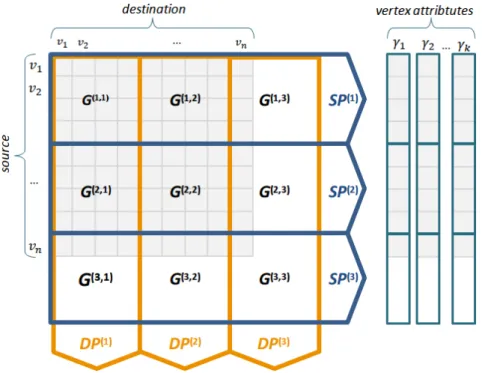
Figure 8 – Organization of edges and vertices in M-Flash.Left (edges): example of a graph’s adjacency matrix (in light blue color) organized in M-Flash using 3 logical intervals (β =3);G(p,q) is an edge block
with source vertices in intervalI(p)and destination vertices in intervalI(q);SP(p)is asource-partition contaning all blocks with source vertices in intervalI(p);DP(q)is adestination-partitioncontaning all blocks with destination vertices in intervalI(q).Right (vertices):the data of the vertices askvectors (γ1
...γk), each one divided intoβ logical segments.
Finally, system design and implementation are discussed in Section 3.4.4.
The design of M-Flash considers the fact that real graphs have varying density of edges; that is, a given graph contains dense regions with more edges than other regions that are sparse. In the development of M-Flash, and through experimentation with existing works, we noticed that these dense and sparse regions could not be processed in the same way. We also noticed that this was the reason why existing works failed to achieve superior performance. To cope with this issue, we designed M-Flash to work according to two distinct processing schemes: Dense Block Processing (DBP) and Streaming Partition Processing (SPP). Hence, for full performance, M-Flash uses a theoretical I/O cost to decide the kind of processing for a given block, which can be dense or sparse. The final approach, which combines DBP and SPP, was named Bimodal Block Processing (BBP).
3.4.1
Graphs Representation in M-Flash
A graph in M-Flash is a directed graphG= (V,E)with verticesv∈V labeled with integers from 1 to|V|, and edgese= (source,destination),e∈E. Each vertex has a set of attributes
γ={γ1,γ2, . . . ,γK}.
3.4. M-Flash 47
G (3,3)
Source I(2) Source I(1)
Source I(3)
Destination I(3)
Destination I(2) Destination I(1)
G (2,3)
G (1,3)
G (3,2)
G (2,2)
G (1,2)
G (3,1)
G (2,1)
G (1,1)
Figure 9 – M-Flash’s computation schedule for a graph with 3 intervals. Vertex intervals are represented by vertical (Source I) and horizontal (Destination I) vectors. Blocks are loaded into memory, and processed, in a vertical zigzag manner, indicated by the sequence of red, orange and yellow arrows. This enables the reuse of input (e.g., when going fromG(3,1)toG(3,2), M-Flash reuses source node intervalI(3)), which reduces data transfer from disk to memory, boosting the speed.
where 1≤p≤β. Note thatI(p)∩I(p′)=∅ for p6= p′, andS
p I(p) =V. Thus, as shown in
Figure 8, the edges are divided intoβ2blocks. Each blockG(p,q)has a source node interval pand a destination node intervalq, where 1≤ p,q≤β. In Figure 8, for example, G(2,1) is the block that contains edges with source vertices in the intervalI(2) and destination vertices in the intervalI(1). In total, we haveβ2blocks. We call this on-disk organization of the graph as
partitioning. Since M-Flash works by alternating one entire block in memory for each running thread, the value ofβ is automatically determined by equation:
β =
2φT|V| M
(3.1)
in which, M is the available RAM, |V| is the total number of vertices in the graph,φ is the amount of data needed to store each vertex, and T is the number of threads. For example, for 1 GB RAM, a graph with 2 billion nodes, 2 threads, and 4 bytes of data per node, β =
⌈(2×8×2×2∗109)/(230)⌉=30, thus requiring 302=900 blocks.
3.4.2
The M-Flash Processing Model
This section presents our proposed M-Flash. We first describe two strategies targeted at processing dense and sparse blocks. Next, we explain the cost-based optimization of M-Flash to take the best of them.
48 Chapter 3. M-Flash: Fast Billion-scale Graph Computation Using a Bimodal Block Processing Model
Figure 10 – Example I/O operations to process thedenseblockG(2,1).
partitioning the graph intoblocks, we process them in a vertical zigzag order, as illustrated in Figure 9. There are three reasons for this order: (1) we store the computation results in the destination vertices; so, we can “pin” a destination interval (e.g.,I(1)) and process all the vertices that are sources to this destination interval (see the red vertical arrow); (2) using this order leads to fewer reads because the attributes of the destination vertices (horizontal vectors in the illustration) only need to be read once, regardless of the number of source intervals. (3) after reading all the blocks in a column, we take a “U turn” (see the orange arrow) to benefit from the fact that the data associated with the previously-read source interval is already in memory, so we can reuse that.
Within a block, besides loading the attributes of the source and destination intervals of vertices into RAM, the corresponding edgese=hsource,destination,edge propertiesiare sequentially read from disk, as explained in Fig. 10. These edges, then, are processed using a user-defined function so to achieve a given desired computation. After all blocks in a column are processed, the updated attributes of the destination vertices are written to disk.
Streaming Partition Processing (SPP): The performance of DBP decreases for graphs with very low density (sparse) blocks; this is because, for a given block, we have to read more data from the source intervals of vertices than from the very blocks of edges. For such situations, we designed the technique namedStreaming Partition Processing (SPP). The SPP processes a given graph using partitions instead of blocks. A graphpartitioncan be a set ofblockssharing the samesource node interval– a line in the logical partitioning, or, similarly, a set ofblocks
sharing the samedestination node interval– a column in the logical partitioning. Formally, a
source-partition SP(p)=S
qG(p,q) contains all blocks with edges having source vertices in the
intervalI(p); a destination-partition DP(q) =S
pG(p,q) contains all blocks with edges having
destination vertices in the intervalI(q). For example, in Figure 8,DP(3) is the union of the blocks
3.4. M-Flash 49
Figure 11 – Example I/O operations for step 1 ofsource-partitionSP3. Edges of SP1are combined with their source
vertex values. Next, the edges are divided byβ destination-partitionsin memory; and finally, edges are written to disk. On Step 2 ,destination-partitionsare processed sequentially. Example I/O operations for step 2 ofdestination-partitionDP(1).
For processing the graph usingSPP, we divide the graph inβ source-partitions. Then, we process partitions using a two-step approach (see Fig. 11). In the first step for each source-partition, we load vertex values of the intervalI(p); next, we read edges of the partitionSP(p)
sequentially from disk, storing in a temporal buffer edges together with their in-vertex values until the buffer is full. Later, we shuffle the buffer in-place, grouping edges bydestination-partition. Finally, we store to disk edges inβ different files, one bydestination-partition. After we process theβ source-partitions, we getβ destination-partitionscontaining edges with their source values. In the second step for eachdestination-partition, we initialize vertex values of intervalI(q); next, we read edges sequentially, processing their values through a user-defined function. Finally, we store vertex values of intervalI(q)on disk. TheSPPmodel is an improvement of the edge streaming approach used in X-Stream [11]; different from former proposals, SSP uses only one buffer to shuffle edges, reducing memory requirements.
Bimodal Block Processing (BBP): SchemesDBPandSPPimprove the graph performance in opposite directions.
• how can we decide which processing scheme to use when we are given a graph block to process?