www.solid-earth.net/5/1055/2014/ doi:10.5194/se-5-1055-2014
© Author(s) 2014. CC Attribution 3.0 License.
Fully probabilistic seismic source inversion – Part 1: Efficient
parameterisation
S. C. Stähler1and K. Sigloch1,2
1Dept. of Earth and Environmental Sciences, Ludwig-Maximilians-Universität (LMU), Munich, Germany 2Dept. of Earth Sciences, University of Oxford, South Parks Road, Oxford OX1 3AN, UK
Correspondence to:S. C. Stähler ([email protected]) Received: 3 July 2013 – Published in Solid Earth Discuss.: 23 July 2013
Revised: 14 October 2013 – Accepted: 28 October 2013 – Published: 17 November 2014
Abstract. Seismic source inversion is a non-linear prob-lem in seismology where not just the earthquake param-eters themselves but also estimates of their uncertainties are of great practical importance. Probabilistic source in-version (Bayesian inference) is very adapted to this chal-lenge, provided that the parameter space can be chosen small enough to make Bayesian sampling computationally feasi-ble. We propose a framework for PRobabilistic Inference of Seismic source Mechanisms (PRISM) that parameterises and samples earthquake depth, moment tensor, and source time function efficiently by using information from previ-ous non-Bayesian inversions. The source time function is expressed as a weighted sum of a small number of empir-ical orthogonal functions, which were derived from a cata-logue of >1000 source time functions (STFs) by a princi-pal component analysis. We use a likelihood model based on the cross-correlation misfit between observed and predicted waveforms. The resulting ensemble of solutions provides full uncertainty and covariance information for the source pa-rameters, and permits propagating these source uncertainties into travel time estimates used for seismic tomography. The computational effort is such that routine, global estimation of earthquake mechanisms and source time functions from teleseismic broadband waveforms is feasible.
1 Introduction
Seismic source inversion is one of the primary tasks of seis-mology, and the need to explain devastating ground move-ments was at the origin of the discipline. The interest is to locate the earthquake source using seismogram recordings,
and to combine this information with geological knowledge, in order to estimate the probability of further earthquakes in the same region. This purpose is served well by a vari-ety of existing source catalogues, global and regional. Large earthquakes and those in densely instrumented areas are be-ing studied in detail, usbe-ing extended-source frameworks like finite-fault or back-projection.
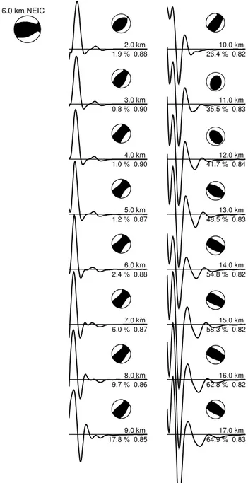
A few recent catalogues now include STF estimates (Vallée et al., 2011; Garcia et al., 2013), but the treatment of parameter uncertainties is still incomplete. Uncertain-ties in the STF correlate most strongly with source depth estimates, especially for shallow earthquakes (Sigloch and Nolet, 2006), where surface-reflected phases (pP, sP) in-evitably enter the time window for STF estimation (see Fig. 1). Inversion for the STF and the moment tensor is linear, whereas inversion for depth is inherently non-linear. Hence gradient-free optimisation techniques like simulated anneal-ing (Kirkpatrick et al., 1983) or the first stage of the neigh-bourhood algorithm (NA) (Sambridge, 1999a) have become popular; Table 4 presents an overview of gradient-free source inversion algorithms from recent years. These optimisation algorithms provide only rudimentary uncertainty estimates.
A natural alternative, pursued here, is Bayesian sampling, where an ensemble of models is generated. The members of this ensemble are distributed according to the posterior probability densityP (m), wherem is the model parameter vector to estimate. Integrating over certain parameters of this joint posterior P (m), or linear combinations thereof, yields marginal distributions over arbitrary individual parameters or parameter combinations. To the best of our knowledge, en-semble sampling in the context of source parameter estima-tion has been tried twice so far (Wéber, 2006; Deb¸ski, 2008), and has been limited to a few events in either case.
A hurdle to using sampling algorithms has been the ef-ficient parameterisation of the source time function. We propose a parameterisation based on empirical orthogonal wavelets (Sect. 2.1), which reduces the number of free pa-rameters to less than 12 for the STF, and to around 18 in to-tal. We show that this makes Bayesian sampling of the entire model space computationally feasible.
A normalised moment tensor is sampled explicitly, and the scalar moment and absolute values for Mj are derived
from the amplitude misfit (Sect. 2.2). Section 3 introduces Bayesian inference as a concept and explains the model space and prior assumptions. The ensemble inference is done with the neighbourhood algorithm (Sambridge, 1999a, b). In Sect. 4, the code is applied to a magnitude 5.7 earthquake in Virginia, 2011. Section 5 discusses aspects of our algorithm and potential alternatives, which we compare to related stud-ies by other workers in Sect. 5.4 and in the Appendix.
Our procedure is called PRISM (PRobabilistic Inference of Source Mechanisms); by applying it routinely, we plan to publish ensemble solutions for intermediate-size earthquakes in the near future. A usage of uncertainty information gained from the ensemble is demonstrated in Sect. 4.3, where the influence of source uncertainties on tomographic travel time observables is estimated. Further investigations of noise and of inter-station covariances are presented in a companion pa-per (Stähler et al., 2014).
Figure 1.Source time function solutions for aMW5.7 earthquake in
2 Method
2.1 Parameterisation of the source time function Source time function (STF) is a synonym for the moment rate m(t )˙ of a point source, denoting a time series that de-scribes the rupture evolution of the earthquake. It is related tou(t ), the vertical or transverse component of the displace-ment seismogram observed at location rr by convolution with the Green function:
u(t )= 3 X j=1
3 X k=1
∂Gj
∂xk
(rs,rr, t )∗s(t )·Mj,k, (1)
wheres(t )≡ ˙m(t )is the STF;Mj,kdenotes the elements of
the symmetric, 3×3 moment tensor,M; andG(rs,rr, t )is the Green function between the hypocentre rs and receiver locationrr.
Due to the symmetry of M, we can reduce Eq. (1) to a simpler form:
u(t )= 6 X j=1
gl(t )·s(t )·Ml, (2)
where Ml are the unique moment tensor elements and gl
are the respective derivatives of the Green function. The el-ements gj are not 3-D vectors because we compute either
only its vertical component (for P waves) or its transverse component (for SH waves). In either case,g is a superpo-sition of six partial functionsgj, corresponding to
contribu-tions from six unique moment tensor elements Ml, with a
weighting for the non-diagonal elements ofM, which appear twice in Eq. (1). The orientation of the source is considered to remain fixed during the rupture – i.e.,Mldoes not depend
ont– so that a single time seriess(t )is sufficient to describe rupture evolution.
For intermediate-size earthquakes (5.5< MW<7.0) the STF typically has a duration of several seconds, which is not short compared to the rapid sequence of P–pP–sP or S–sS pulses that shallow earthquakes produce in broadband seismograms. Most earthquakes are shallow in this sense, i.e., shallower than 50 km. In order to assemble tomography-sized data sets, it is therefore imperative to account for the source time function in any waveform fitting attempt that goes to frequencies above ≈0.05 Hz (Sigloch and Nolet, 2006).
Equations (1) and (2) are linear ins(t ), so thats(t )can be determined by deconvolvingg fromuifMj in considered
fixed. However, gdepends strongly on source depth (third component of vectorrs), so that a misestimated source depth will strongly distort the shape of the STF, as demonstrated by Fig. 1. Another complication is present in the fact that ob-served seismogramsu(t )(as opposed to the predicted Green functions) are time-shifted relative to each other due to 3-D heterogeneity in the earth, and should be empirically aligned before deconvolvings(t ).
These issues can be overcome by solving iteratively for s(t ) andMj with a fixed depth (Sigloch and Nolet, 2006;
Stähler et al., 2012), but the approach requires significant hu-man interaction, which poses a challenge for the amounts of data now available for regional or global tomography. More-over, such an optimisation approach does not provide sys-tematic estimates of parameter uncertainties.
Monte Carlo sampling avoids the unstable deconvolution and permits straightforward estimation of full parameter un-certainties and covariances. However, the model space to sample grows exponentially with the number of parameters, and the STF adds a significant number of parameters. In a naive approach, this number could easily be on the order of 100, i.e., computationally prohibitive. For example, the STFs deconvolved in Fig. 1 were parameterised as a time series of 25 s duration, sampled at 10 Hz, and thus yielding 250 un-knowns – not efficient, since neighbouring samples are ex-pected to be strongly correlated. This raises the question of how many independent parameters or degrees of freedom this problem actually has.
Due to intrinsic attenuation of the earth, the high-est frequencies still significantly represented in teleseismic P waves are around 1 Hz. If from experience we require a duration of 25 s to render the longest possible STFs oc-curring for our magnitude range (Houston, 2001), then the time-bandwidth product is 1 Hz·25 s=25, and the problem cannot have more degrees of freedom than that.
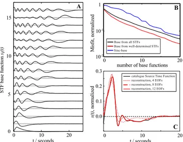
Efficient parameterisation then amounts to finding a basis of not more than 25 orthogonal functions that span the sub-space of the real-world, band-limited STFs just described. In fact, we can empirically decrease the number of parameters even further. By the method of Sigloch and Nolet (2006), we have semi-automatically deconvolved more than 3000 broad-band STFs while building data sets for finite-frequency to-mography. Of these, we propose to use the 1000 STFs that we consider most confidently determined as prior informa-tion for what the range of possible STFs looks like, for earth-quakes of magnitude 5.5< MW<7.5. By performing a prin-cipal component analysis on this large set of prior STFs, we find that only around 10 empirical orthogonal wavelets are needed to satisfactorily explain almost all of the STFs, as shown in Fig. 2.
In concrete terms, we applied the MATLAB function prin-comp.m to a matrix containing the 1000 prior STFs in its rows. The mean over the matrix columns (time samples) was subtracted prior to performing the decomposition, and is shown in Fig. 2a as wavelet s0(t ). Principal component analysis then determiness1(t )as the function orthonormal to s0(t ) that explains as much of the variance in the ma-trix rows as possible. After subtracting (optimally weighted) s1(t )from each row, functions2(t )is determined such that it is orthonormal tos0(t )ands1(t ), and explains as much as possible of the remaining variance. Each subsequent iteration generates another orthonormalsi untili=256, the number
Figure 2.Efficient parameterisation of the STF in terms of empiri-cal orthogonal functions, computed from a large set of manually de-convolved STFs that effectively serve as prior information.(a)First 16 members of the basis of empirical orthogonal functions.(b) Me-dian RMS misfit between members of the prior STF catalogue and their projection on a subspace of the model space spanned by the first wavelet basis functions.(c)A typical STF from the catalogue, and its projection onto several subspaces spanned by the first few basis functions (N= [4,8,12]).
can now be expressed as
s(t )= 256 X i=1
aisi(t )+s0(t ). (3)
In this parameterisation, the new unknowns to solve for dur-ing source estimation are theai. Since principal component
analysis has sorted theai by their importance to explaining
a typical STF, we may choose to truncate this sum at a rela-tively low valueN≪256:
sN(t )= N X i=1
aisi(t )+s0(t ). (4)
In practice, N will be chosen based on the residual misfit between s(t )andsN(t )that one is willing to tolerate.
Fig-ure 2b shows the dependence of this misfit onN. If we tol-erate an average root mean square (RMS) misfit of 10 % in total signal variance, N=10 base functions are sufficient, compared to 16, when using asincbase. In the following we useN=12.
A set of potentially problematic STFs expressed by our base functions is shown in an electronic supplement to this paper.
2.2 Parameterisation of the moment tensor
The orientation of the source can be parameterised either by a moment tensor using 6 parameters or as a pure shear
displacement source (Aki and Richards, 2002, p. 112) with strike, slip and dip (to which a term for an isotropic com-ponent might be added). Here we want to estimate the non-double-couple content of the solutions, and hence we sam-ple the full moment tensor. The scalar moment is fixed to 1, so that only relativeMj are estimated. This is equivalent to
sampling a hypersphere in the six-dimensional vector space
{Mxx, Myy, Mzz, Mxy, Myz, Mxz}with
M0 = 1
√
2 q
M2
xx+Myy2 +Mzz2 +2(Mxy2 +Myz2 +Mxz2)
= 1. (5)
Uniform sampling on a n-D hypersphere can be achieved by the method of Tashiro (1977), which transforms n−1 uniformly distributed random variablesxi to producen
ran-dom variablesri that are distributed uniformly on a
hyper-sphere with q
P6
i=1ri2=1. We identifyri with the moment
tensor components and note that the non-diagonal elements Mkl, k6=lappear twice in the sum (thus we actually sample
an ellipsoid rather than a hypersphere). We then have xi∼U (0,1), i=1,2, . . . ,5
Y3=1; Y2=√x2; Y1=Y2x1
Mxx/M0= p
Y1·cos(2π x3)
√
2 Myy/M0=
p
Y1·sin(2π x3)
√
2 (6)
Mzz/M0= p
Y2−Y1·cos(2π x4)
√
2 Mxy/M0=
p
Y2−Y1·sin(2π x4) Myz/M0=
p
Y3−Y2·cos(2π x5) Mzx/M0=
p
Y3−Y2·sin(2π x5) 2.3 Forward simulation
3 Source parameter estimation by Bayesian sampling 3.1 Bayesian inversion
Bayesian inversion is an application of Bayes’ rule:
P (m|d)=P (d|m)P (m)
P (d) , (7)
wheremis a vector of model parameters (in our case depth, moment tensor elementsMj and STF weightsai), andd is
a vector of data, i.e., a concatenation of P and SH wave-forms. These quantities are considered to be random vari-ables that follow Bayes’ rule. We can then identify P (m) with the prior probability density of a model. This is the in-formation on the model parameters that we have independent of the experiment. The conditional probability ofdgivenm, P (d|m), also calledL(m|d), is thelikelihoodof a modelm
to produce the datad. TermP (d)is constant for all models and is therefore dropped in what follows.P (m|d)is called the posterior probability density (short, “the posterior”) and denotes the probability assigned to a model mafter having done the experiment.
P (m|d)=P (m)L(m|d)k−1 (8) Since the posteriorP (m|d)may vary by orders of magnitude for differentd, we work with its logarithm. We introduce the quantity8(m|d)to denote some kind of data misfit such that the likelihood can be written asL(m)=exp[−8(m|d)]. ln(P (m|d))= −8(m|d)+lnP (m)−lnk (9) The normalisation constantkis
k= Z
exp[−8(m|d)]P (m)dm (10) and calculated by the neighbourhood algorithm in the ensem-ble inference stage.
In the case of multivariate, Gaussian-distributed noise on the data with a covariance matrixSD,
d=g(m)+ǫ, ǫ∼N(0,SD), (11)
whereg(m)is the data predicted by modelm, we would ob-tain the familiar expression
8(m|d)=k′
1
2(d−g(m))
TS−1
D (d−g(m))
. (12)
This term is usually called Mahalanobis distance orℓ2-misfit. We do not choose this sample-wise difference between ob-served and predicted waveforms as our measure of misfit. There are questions about the Gaussian noise assumption for real data, but mainly we consider there to be a measure that is more robust and adapted to our purpose, the cross-correlation (mis-)fit between data and synthetics (Stähler et al., 2014),
which essentially quantifies phase misfit. In the optimisation-based, linearised approach to tomography, fitting the phase shift between two waveforms remains a near-linear problem in a wider range around the reference model than fitting the waveforms sample-wise. The cross-correlation fit is defined as
CC(1Ti)=
R t u
c
i(t−1Ti)·ui(t )dt
q R
t u c
i(t−1Ti) 2
dt· q
R
t(ui(t−1Ti))2dt
, (13)
whereui(t )is the measured anduci(t )is the synthetic
wave-form for a modelmat stationi. In general,CCis a function of the time lag1Ti for which we compare the observed and
predicted waveforms, but here we imply that1Tihas already
been chosen such as to maximiseCC(1Ti). (This value of
1Tithat maximises the cross-correlation is called the
“finite-frequency travel time anomaly” of waveformui(t ), and
rep-resents the most important observable for finite-frequency tomography (Nolet, 2008; Sigloch and Nolet, 2006). Sec-tion 4.3, which discusses error propagaSec-tion from source in-version into tomographic observables, further clarifies this motivation of the cross-correlation criterion further.)
Correlation CC(1Ti) measures goodness of fit, so we
choose decorrelationDi=1−CC(1Ti)as our measure of
misfit (one scalar per wave pathi). From the large set of pre-existing deterministic source solutions described in Sect. 2.1, we estimated the distribution of this misfit Di, based on
our reference data set of about 1000 very confidently de-convolved STF solutions. For this large and highly quality-controlled set of earthquakes, we empirically find that the decorrelation Di of its associated seismograms ui(t ) and
uci(t ) follows a log-normal distribution in the presence of the actual noise and modelling errors. The statistics of this finding are discussed further in the companion paper (Stähler et al., 2014), but here we use it to state our likelihood func-tionL, which is the multivariate log-normal distribution:
L=exp
−12(ln(D)−µ) TS−1
D (ln(D)−µ) (2π )n2√|det(SD)|
. (14)
Dis the decorrelation vector into whichndecorrelation coef-ficientsDi are gathered. EachDi was measured on a pair of
observed/predicted broadband waveforms that contained ei-ther aP or an SH arrival. The parameters of this multivariate log-normal distribution are its mean vectorµcontaining n meansµi and its covariance matrixSD. Empirically we find
that theµiand the standard deviationsσi(diagonal elements
ofSD) depend mainly on the signal-to-noise-ratio (SNR) of
waveformui. The data covariance between two stationsiand
j (off-diagonal elements inSD) is predominantly a function
of the distance between stationiand stationj. We estimate their values from the data set of the 1000 trustworthy STF so-lutions, i.e., from prior information, and proceed to use these
It follows from Eq. (14) that the misfit8is
8 = 1
2
n X
i n X
j
ln(Dj)−µjTSD,ij−1 ln(Dj)−µj !
+ 1
2ln (2π )
n
|det(SD)| (15)
3.2 Construction of the prior probability density A crucial step in Bayesian inference is the selection of prior probabilitiesP (m)on the model parametersm. Our model parameters are as follows:
– m1: source depth. We assume a uniform prior based on the assumed depth of the event in the National Earthquake Information Center (NEIC) catalogue. If the event is shallow according to the International Seismological Centre (ISC) catalogue (<30 km), we draw from depths between 0 km and 50 km; i.e.,m1∼
U(0,50). For deeper events, we draw from depths
be-tween 20 km and 100 km. Events deeper than 100 km have to be treated separately, using a longer time win-dow in Eq. (13) that includes the surface reflected phasespPandsP.
– m2, . . . , m13=a1, . . . , a12: the weights of the source time function (Eq. 4). The samples are chosen from uni-form distributions with ranges shown in Table 1, but are subjected to a prior,πSTF(see below).
– m14, . . . , m18=x1, . . . x5: the constructor variables for the moment tensor (Eq. 6). xi∼U(0,1), but they are
subjected to two priors,πisoandπCLVD(see below). Intermediate-sized and large earthquakes are caused by the release of stress that has built up along a fault, driven by shear motion in the underlying, viscously flowing mantle. Hence the rupture is expected to proceed in only one direc-tion, the direction that releases the stress. The source time function is defined as the time derivative of the moment, s(t )= ˙m(t ). The moment is proportional to the stress and thus monotonous, and hence s(t ) should be non-negative. In practice, an estimated STF is often not completely non-negative (unless this characteristic was strictly enforced). The reason for smaller amounts of “negative energy” (time samples with negative values) in the STF include reverber-ations at heterogeneities close to the source, which produce systematic oscillations that are present in most or all of the observed seismograms. Motivated by waveform tomography, our primary aim is to fit predicted to observed waveforms. If a moderately non-negative STF produces better-fitting syn-thetics, then our pragmatic approach is to accept it, since we are not interested in source physics per se. However, we still need to moderately penalise non-negative samples in the STF, because otherwise they creep in unduly when the prob-lem is underconstrained, due to poor azimuthal receiver cov-erage. In such cases, severely negative STFs often produce
Table 1.Sampling of the prior probability distribution: range of STF weightsai that are permitted in the first stage of the neighbourhood algorithm.
i Range i Range i Range
1 ±1.5 7 ±0.8 12 ±0.5 2 ±1.0 8 ±0.7 13 ±0.5 3 ±0.9 9 ±0.7 14 ±0.4 4 ±0.8 10 ±0.6 15 ±0.4
marginally better fits by fitting the noise. Smaller earthquakes in other contexts, like mining tremors or dyke collapse in volcanic settings, may have strong volume changes involved and therefore polarity changes in the STF (e.g. Chouet et al., 2003). However, such events are outside of the scope of this study.
Our approach is to punish slightly non-negative STF esti-mates only slightly, but to severely increase the penalty once the fraction of “negative energy”I exceeds a certain thresh-oldI0. To quantify this, we defineI as the squared negative part of the STF divided by the entire STF squared:
I= RT
0 sN(t )2·2(−sN(t ))dt RT
0 sN(t )2
, where (16)
sN=s0(t )+ N X i=1
aisi(t ) (17)
and 2 is the Heaviside function. Based on I, we define a priorπSTF:
πSTF(m2, . . . , m13)=exp "
−
I I0
3#
, (18)
where the third power andI0=0.1 have been found to work best. In other words, up to 10 % of STF variance may be contributed by negative samples (mostly oscillations) with-out penalty, but any larger contribution is strongly penalized by the priorπSTF.
The neighbourhood algorithm supports only uniform dis-tributions on parameters. The introduction ofπSTF defined by Eq. (18) leads to a certain inefficiency, in that parts of the model space are sampled that are essentially ruled out by the prior. We carefully selected the ranges of theai by
examin-ing their distributions for the 1000 catalogue solutions. A test was to count which fraction of random models were consis-tent withI <0.1. For the ranges given in Table 1, we found that roughly 10 % of the random STF estimates hadI <0.1. A second prior constraint is that earthquakes caused by stress release on a fault should involve no volume change, meaning that the isotropic componentMiso=Mxx+Myy+
Mzzof the moment tensor should vanish. Hence we introduce
πiso(m14, . . . , m18)=exp "
−
M
iso/M0 σiso
3#
, (19)
whereM0is the scalar moment, andσiso=0.1 is chosen em-pirically.
Third, we also want to encourage the source to be double-couple-like. A suitable prior is defined on the compensated linear vector dipole (CLVD) content, which is the ratio ǫ=
|λ3|/|λ1|between smallest and largest deviatoric eigenvalues of the moment tensor:
πCLVD(m14, . . . , m18)=exp "
−
ǫ
σCLVD 3#
. (20)
In the absence of volume change, a moment tensor with ǫ=0.5 corresponds to a purely CLVD source, whileǫ=0 is a pure DC source. Again we have to decide on a sensi-ble value for the characteristic constant σCLVD. We choose σCLVD=0.2, which seems to be a reasonable value for the intermediate-sized earthquakes of the kind we are interested in (Kuge and Lay, 1994).
The total prior probability density is then
P (m)=πSTF(m2, . . . , m13) (21)
+πiso(m14, . . . , m18)+πCLVD(m14, . . . , m18). 3.3 Sampling with the neighbourhood algorithm Our efficient wavelet parameterisation of the STF reduces the total number of model parameters to around 18, but sam-pling this space remains non-trivial. The popular Metropolis– Hastings algorithm (MH) (Hastings, 1970) can handle prob-lems of this dimensionality, but is non-trivial to use for sam-pling multimodal distributions (see the discussion for de-tails). These problems are less severe for a Gibbs sampler, but this algorithm needs to know the conditional distribu-tionp(xj|x1, . . . xj−1, xj+1, xn)along parameterxj in the
n-dimensional model space (Geman and Geman, 1984). This conditional distribution is usually not available, especially not for non-linear inverse problems.
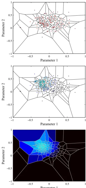
To overcome the problem of navigation in complex high-dimensional model spaces, the neighbourhood algorithm uses Voronoi cells (Sambridge, 1998) to approximate a map of the misfit landscape (Sambridge, 1999a, first stage), fol-lowed by a Gibbs sampler to appraise an ensemble based on this map (Sambridge, 1999b, second stage).
In order to point the map-making first stage of the NA into the direction of a priori allowed models, we use a pre-calculated set of starting models. For that, the NA is run with-out forward simulations and withwith-out calculating the likeli-hood, so that only a map of the prior landscape is produced, from 32 768 samples (Fig. 3a). This means that from the start the map will be more detailed in a priori favourable regions, and avoids the algorithm wasting too much time refining the map in regions that are essentially ruled out by the prior.
−1 −0.5 0 0.5 1
−1 −0.5 0 0.5 1
Parameter 1
Parameter 2
−1 −0.5 0 0.5 1
−1 −0.5 0 0.5 1
Parameter 1
Parameter 2
−1 −0.5 0 0.5 1
−1 −0.5 0 0.5 1
Parameter 1
Parameter 2
Next, the prior landscape is loaded and a forward simula-tion is run for each member in order to evaluate its posterior probability. Then this map is further refined by 512 forward simulations around the 128 best models. This is repeated un-til a total of 65 536 models have been evaluated.
In the second stage of the NA, which is the sampling stage, 400 000 ensemble members are drawn according to the pos-terior landscape from the first step. This process runs on a 16-core Xeon machine and takes around 2 h in total per earthquake.
4 A fully worked example
4.1 2011/08/23 Virginia earthquake
In the following we present a fully worked example for a Bayesian source inversion, by applying our software to the MW 5.7 earthquake that occurred in central Virginia on 23 August 2011 (Figs. 4 and 5, also compare to Fig. 1). While not considered a typical earthquake region, events from this area have nevertheless been recorded since the early days of quantitative seismology (Taber, 1913). Due to its occur-rence in an unusual but densely populated area, this relatively small earthquake was studied in considerable detail, afford-ing us the opportunity to compare to results of other workers. Moderate-sized events of this kind are typical for our tar-geted application of assembling a large catalogue. The great-est abundance of suitable events is found just below magni-tude 6; toward smaller magnimagni-tudes, the teleseismic signal-to-noise ratio quickly deteriorates below the usable level.
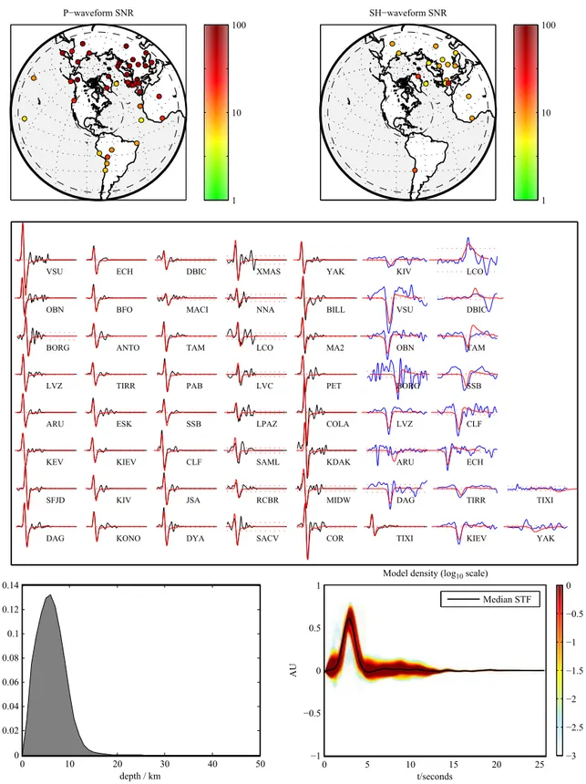
For the inversion, we used a set of 41P waveforms and 17 SH waveforms recorded by broadband stations at teleseismic distances (Fig. 4). For waveform modelling, a simplified ver-sion of the crustal model CRUST2.0 (Bassin et al., 2000) was assumed around the source region. Layers 3-5 of CRUST2.0 were averaged into one layer above the Conrad discontinuity, and layers 6-7 were averaged into one layer from the Con-rad discontinuity to the Moho; the resulting values are given in Table 2. The algorithm ran 65 536 forward simulations to generate a map of the posterior landscape, and produced an ensemble of 400 000 members in the second step. From this ensemble, the source parameters were estimated. Table 3 shows the estimated credible intervals and the median of the probability distribution for the depth and the moment ten-sor. These quantiles represent only a tiny part of the infor-mation contained in the ensemble, i.e., two statistics of 1-dimensional marginals derived from a 16-1-dimensional prob-ability density function. Some credible intervals are large; for example we cannot constrain the depth to a range nar-rower than 10 km with 90 % credibility. Using such credible interval estimates, routine production runs of our software should be able to clarify whether depth uncertainties in ex-isting catalogues tend to be overly optimistic or pessimistic.
Table 2.Crustal model assumed for the source region of the 2011 Virginia earthquake (CRUST2.0).
VP VS ρ Depth
Upper 4.10 km s−1 2.15 km s−1 2.51 Mg m−3 10.5 km crust
Lower 6.89 km s−1 3.84 km s−1 2.98 Mg m−3 24.5 km crust
Table 3.Credible intervals for source parameters of the Virginia earthquake. The moment tensor componentsMklneed to be multi-plied by 1016Nm.
1st decile Median 9th decile
Depth 1.8 5.9 11
MW 5.57 5.67 5.74
Myy −0.233 1.38 2.54
Mxy −1.99 −0.955 −0.165
Mxz −2.7 −0.325 2.72
Myy −9.4 −4.74 −2.7
Mzy −3.25 −0.563 1.87
Mzz 3.16 4.42 7.84
The complete marginal distribution of the source depth esti-mate is shown in Fig. 3, bottom left.
We aim for additional, informative ways of summarising and conveying the resulting ensemble. Figure 5 is what we call a “Bayesian beach ball”: an overlay of 1024 focal mech-anisms drawn from the ensemble at random. The thrust fault-ing character of the event is unambiguous, but the direction of slip is seen to be less well constrained. The estimate of the source time function and its uncertainty are displayed in Fig. 4, bottom right. Within their frequency limits, our tele-seismic data prefer a single-pulsed rupture of roughly 3 s du-ration, with a certain probability of a much smaller foreshock immediately preceding the main event. Smaller aftershocks are possible, but not constrained by our inversion.
P−waveform SNR
1 10
100 SH−waveform SNR
1 10 100
DAG SFJD KEV ARU LVZ BORG OBN VSU
KONO KIV KIEV ESK TIRR ANTO BFO ECH
DYA JSA CLF SSB PAB TAM MACI DBIC
SACV RCBR SAML LPAZ LVC LCO NNA XMAS
COR MIDW KDAK COLA PET MA2 BILL YAK
TIXI DAG ARU LVZ BORG OBN VSU KIV
KIEV TIRR ECH CLF SSB TAM DBIC LCO
YAK TIXI
0 10 20 30 40 50
0 0.02 0.04 0.06 0.08 0.1 0.12 0.14
depth / km
ppd
0 5 10 15 20 25
−1 −0.5 0 0.5 1
t/seconds
AU
Model density (log10scale)
−3 −2.5 −2 −1.5 −1 −0.5 0 Median STF
Figure 4.Waveform data and source estimates for the 2011/08/23 Virginia earthquake (MW5.7). Top row: distribution of 41 and 17
teleseis-mic broadband stations that recordedP andSwaveforms, respectively. Station colour corresponds to the signal-to-noise ratio in the relevant waveform window. Middle row: synthetic broadband waveforms (red), compared to the data for the best-fitting model. Black waveforms are
Figure 5.Bayesian beach ball: probabilistic display of focal mech-anism solutions for the 2011 Virginia earthquake.
50 % higher than ours, which may explain why he estimates the source 1–2 km deeper than our most probable depth of 5.9 km (Fig. 4, bottom left).
4.3 Uncertainty propagation into tomographic observables
We are interested in source estimation primarily because we want to account for the prominent signature of the source wavelet in the broadband waveforms that we use for wave-form tomography. Input data for the inversion, primarily travel time anomalies1Ti, whereiis the station index, are
generated by cross-correlating observed seismograms with predicted ones. A predicted waveform consists of the con-volution of a synthetic Green’s function with an estimated source time function (Eq. 2). Thus uncertainty in the STF estimate propagates into the cross-correlation measurements that generate our input data for tomography. Previous ex-perience has led us to believe that the source model plays a large role in the uncertainty of1Ti. The probabilistic
ap-proach presented here permits the quantification of this in-fluence by calculating 1Ti,j for each ensemble memberj.
From all values for one station, the ensemble mean1Ti and
its standard deviationσi can then be used as input data for
the tomographic inversion. Thus we obtain a new and robust observable: Bayesian travel time anomalies with full uncer-tainty information.
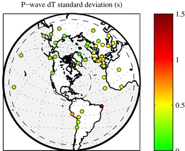
Figure 6 shows the standard deviationσi ofP wave1Ti
at all stations. Comparison to the signal-to-noise ratios of Fig. 6 shows no overall correlation, except for South Amer-ican stations, where a higher noise level is correlated with
P−wave dT standard deviation (s)
0 0.5 1 1.5
Figure 6.Standard deviationsσi ofP wave travel times1Ti, as calculated from the ensemble of solutions. The travel time estimates are by-products of using waveform cross-correlation as the measure for goodness of fit, and they represent our main input data for tomo-graphic inversions. The unit on the colour scale is seconds.
a somewhat larger uncertainty on1Ti. By contrast,
Euro-pean stations all have good SNR, but uncertainties in the travel times are large nonetheless, because source uncertainty happens to propagate into the estimates of1Timore severely
in this geographical region. This information would not have been available in a deterministic source inversion and could strongly affect the results of seismic tomography.
5 Discussion
5.1 Performance of the empirical orthogonal basis for STF parameterisation
events are no more valuable than smaller ones (often quite the opposite, since the point source approximation starts to break down for large events). For a detailed display of a set of po-tentially problematic STFs see the electronic supplement to this paper.
At first glance it might seem unintuitive that the basis func-tions have oscillatory character and thus negative parts, rather than resembling a set of non-negative basis functions (a set of triangles would be one such set). However, the training collection to which the principal components analysis was applied did consist of predominantly non-negative functions, which by construction are then represented particularly effi-ciently, even if the eofs may not give this appearance. On top of this, we explicitly encourage non-negativity of the solu-tion via the priorπSTF(Eq. 18). A rough estimation showed that roughly 90 % of the model space are ruled out by the condition that the source should have a vanishing negative part.
We wanted to know how many basis functions of a more generic basis (e.g., wavelets) would be required in order to approximate the STF collection equally well as with the eofs. A trial with a basis of sinc wavelets showed that 16 basis functions were needed to achieve the same residual misfit as delivered by our optimised basis of only 10 eofs. Since the size of the model space grows exponentially with the number of parameters, avoiding 6 additional parameters makes a big difference in terms of sampling efficiency.
5.2 Moment tensor parameterisation
The parameterisation of the moment tensor is a technically non-trivial point. We discuss the pros and cons of possible alternatives to our chosen solution:
– Parameterisation in terms of strikeφf, slipλand dipδ
is problematic for sampling. Strike and dip describe the orientation of the fault plane; an equivalent description would be the unit normal vectornon the fault.
n=
−sinδsinφf −sinδcosφf
cosδ
(22)
All possible normal vectors form a unit sphere. In or-der to sample uniformly on this unit sphere, samples have to be drawn from a uniform volumetric density (Tarantola, 2005, 6.1). Since the neighbourhood algo-rithm (and most other sampling algoalgo-rithms) implicitly assume Cartesian coordinates in the model space, the prior density has to be multiplied by the Jacobian of the transformation into the actual coordinate system, in our case 1/sinδ. To our knowledge, this consideration is neglected in most model space studies, but it would be more severe in ensemble sampling than in gradient-based optimisation.
– A different issue with strike-dip parameterisation is the following: the Euclidean distances applied to{φf, λ, δ}
by the NA and similar, Cartesian-based algorithms are in fact a rather poor measure of the similarity of two double-couple sources. A more suitable measure of mis-fit is the Kagan angle (Kagan, 1991), which is the small-est angle required to rotate the principal axes of one double couple into the corresponding principal axes of the other, or the Tape measure of source similarity (Tape and Tape, 2012).
This is an issue in model optimisation with the first stage of the neighbourhood algorithm (Kennett et al., 2000; Sambridge and Kennett, 2001; Vallée et al., 2011). Wathelet (2008) has introduced complex boundaries to the NA, but unfortunately no periodic ones.
– An alternative would be to sample {Mxx, Myy, Mzz,
Mxy, Myz, Mxz}independently, but this is inefficient
be-cause the range of physically sensible parameters spans several orders of magnitude.
– Finally, one might choose not to sample the moment tensor at all. Instead, one might sample only from the
{Si, d} model space, followed by direct, linear
inver-sion of the six moment tensor elements corresponding to each sample. This would speed up the sampling con-siderably since the dimensionality of the model space would be reduced from 16 to 10. Moment tensor inver-sion is a linear problem (Eq. 2), and hence we would not lose much information about uncertainties. In a poten-tial downside, moment tensor inversion can be unstable in presence of noise or bad stations, but from our ex-perience with supervised, linear inversions, this is typi-cally not a severe problem in practice. Therefore we are considering this pragmatic approach of reduced dimen-sionality for production runs.
5.3 Neighbourhood algorithm
The neighbourhood algorithm avoids some of the pitfalls of other sampling algorithms. Compared to the popular Metropolis–Hastings algorithm, we see several advantages for our problem:
– The MH is difficult to implement for multivariate distri-butions. This is especially true when the parameters are different physical quantities and follow different distri-butions as is the case in our study.
– As the MH is a random-walk algorithm, the step width is a very delicate parameter. It affects the convergence rate and also the correlation of models, which has to be taken into account when estimating probability density functions from the ensemble. This is a bigger problem than for the Gibbs sampler, which the NA is based on. – The MH is rather bad at crossing valleys of low
These problems are less severe for a Gibbs sampler, on which the second stage of the NA is based.
The first stage of the NA could be replaced by a completely separate mapping algorithm, like genetic algorithms or sim-ulated annealing. Like the first stage of the NA, they only ex-plore the model space for a best-fitting solution. Their results might be used as input for the second stage of the NA. Com-pared to those, the NA has the advantage of using only two tuning parameters, which control (a) how many new mod-els are generated in each step and (b) in how many different cells these models are generated. As in every optimisation al-gorithm, they control the tradeoff between exploration of the model space and exploitation of the region around the best models.
There is no hard-and-fast rule for choosing values for these tuning parameters. Since we do not want to optimise for only one “best” solution, we tend towards an explorative strategy and try to map large parts of the model space. Compared to other source inversion schemes, we are explicitly interested in local minima in the misfit landscape. Local minima are often seen as nuisance, especially in the rather aggressive it-erative optimisation frameworks, but in our view they contain valuable information. What may appear as a local minimum to the specific data set that we are using for inversion might turn out to be the preferred solution of another source inver-sion method (e.g., surface waves, GPS or InSAR).
However, an ensemble that does not resolve the best-fitting model is equally useless. The posterior of all models gets normalised after all forward simulations have been done (see Eq. 10). If one peak (the best solution) is missing, the normal-isation constant k will be too small, and thereforeP (m|d) will be too high for all other models, meaning that the credi-bility bounds will be too large. It is possible that other sam-pling schemes, such asparallel tempering, might find better compromises between exploration and exploitation, which could be a topic of further study.
5.4 Comparison with other source inversion schemes Table 4 shows a list of other point source inversion algo-rithms proposed and applied over the past 15 years. Most widely used is probably the Global Centroid Moment Tensor (CMT) catalogue (Dziewo´nski et al., 1981; Ekström et al., 2012), which is mostly based on intermediate-period (>40 s) waveforms to determine a centroid moment tensor solution. Its results are less applicable to short-period body wave studies, since waveforms in the latter are dominated by the hypocentre, which may differ significantly from the centroid. Another classical catalogue is the ISC bulletin (Bondár and Storchak, 2011), which goes back as far as 1960. The ISC catalogue focuses on estimating event times and locations, neither of which are the topic of this study. The ISC recently adopted a global search scheme based on the first stage of the NA, similar to Sambridge and Kennett (2001), followed by an attempt to refine the result by linearised inversion,
including inter-station covariances. Garcia et al. (2013) and Tocheport et al. (2007) use simulated annealing to infer depth and moment tensor. A STF is estimated from theP wave-forms. By neglecting all crustal contributions and reducing the forward simulation to mantle attenuation, this approach is very efficient.
Similarly, Koláˇr (2000) used a combination of simulated annealing and bootstrapping to estimate uncertainties of the moment tensor, depth and a source time function. The study was limited to two earthquakes.
Kennett et al. (2000) used the first stage of the NA to opti-mise for hypocentre depth, moment tensor, and the duration of a trapezoidal STF, using essentially the same kind of data as the present study, and an advanced reflectivity code for for-ward modelling. However, no uncertainties were estimated.
Deb¸ski (2008) is one of the only two studies, to our knowl-edge, obtained source time functions and their uncertainties by Bayesian inference. He studied magnitude 3 events in a copper mine in Poland. By using the empirical Green’s functions (EGF) method, it was not necessary to do an ex-plicit forward simulation. The study was limited to inverting for the STF, which he parameterised sample-wise. This was possible since the forward problem was computationally very inexpensive to solve.
The second sampling study is Wéber (2006), which used an octree importance sampling algorithm to infer probability density functions for depth and moment tensor rate function. The resulting ensemble was decomposed into focal mech-anisms and source time functions, a trivial and non-unique problem (Wéber, 2009). With this algorithm, a cat-alogue of Hungarian seismicity was produced until 2010, but apparently this promising work was not extended to a global context.
C.
Stähler
and
K.
Sigloch:
Bay
esian
sour
ce
in
v
ersion
P
art
1
1067
Table 4.Overview of similar source inversion algorithms.
Name Characteristics Inversion parameters Algorithms
Focus Pro
ba-bilistic
Depth range
Data
Cata-logue
Depth Location Moment tensor
STF Forward
algorithm and model
Inversion algorithm
PRISM (this paper) global yes full waveforms,
P, SH, teleseismic
yes yes no yes yes WKBJ,
IASP91 + crust
NAa, both stages
Tocheport et al. (2007) global no >100 km
waveforms,
P, teleseismic
no no no yes yes none SAb
Garcia et al. (2013) global no full waveforms,
P, teleseismic
no no no yes yes none SA
Marson-Pidgeon and Kennett (2000)
global no full waveforms,
P, SH, SV
no yes no yes duration reflectivity,
ak135 + crust
NA, first stage Sambridge and Kennett
(2001)
global no full travel times,
P,S
no yes yes no no ak135 NA, first
stage ISC (Bondár and
Storchak, 2011)
global no full travel times,
all phases
yes yesc yes no no ak135 NA, first
stage Global CMT (Ekström
et al., 2012)
global no full waveforms,
P,S+ surface
yes yes yes yes no normal
modes Sigloch and Nolet
(2006)
global no full waveforms,
P, teleseismic
no yes no yes yes WKBJ,
IASP91
LSQR, iterative
Koláˇr (2000) global
uncer-tainties
full waveforms,
P, SH, teleseismic
no yes yes strike,
slip, dip
yes reflectivity (?), local model
SA + boot-strapping SCARDEC (Vallée
et al., 2011)
global uncer-tainties
full waveforms,
P, SH, teleseismic
yes yes no strike,
slip, dip
RSTFd reflectivity, IASP91 + crust
NA, first stage
Wéber (2006) local yes shallow waveforms,
P, local
no yes yes yes MTRFe reflectivity,
local model
octree importance sampling
Deb¸ski (2008) local yes shallow waveforms,
P, local
no no no no yes EGFf Metropolis–
Hastings
aNeighbourhood algorithm (Sambridge, 1999b). bSimulated annealing (Kirkpatrick et al., 1983). cBinning allowed.
dRelative STF, one STF per station.
eMoment tensor rate function, one STF per MT component. fEmpirical Green’s functions.
.solid-earth.net/5/1055/
2014/
Solid
Earth,
5,
1055–
1069
,
6 Conclusions
We showed that routine Bayesian inference of source param-eters from teleseismic body waves is possible and provides valuable insights. From clearly stated a priori assumptions, followed by data assimilation, we obtain rigorous uncertainty estimates of the model parameters. The resulting ensemble of a posteriori plausible solutions permits estimating the prop-agation of uncertainties from the source inversion to other observables of practical interest to us, such as travel time anomalies for seismic tomography.
The Supplement related to this article is available online at doi:10.5194/se-5-1055-2014-supplement.
Acknowledgements. We thank M. Sambridge for sharing his expe-rience on Bayesian inference and B. L. N. Kennett and P. Cum-mins for fruitful discussions. P. Käufl introduced the Tape measure to us. M. Vallée and W. Deb¸ski helped improve the paper in the review process. S. C. Stähler was supported by the Munich Cen-tre of Advanced Computing (MAC) of the International Graduate School on Science and Engineering (IGSSE) at Technische Univer-sität München. IGGSE also funded his research stay at the Research School for Earth Sciences at A. N. U. in Canberra, where part of this work was done.
All waveform data came from the IRIS and ORFEUS data management centres.
Edited by: H. I. Koulakov
References
Aki, K. and Richards, P. G.: Quantitative Seismology, vol. II, Uni-versity Science Books, 2002.
Bassin, C., Laske, G., and Masters, G.: The Current Limits of Reso-lution for Surface Wave Tomography in North America, in: EOS Trans AGU, vol. 81, p. F897, 2000.
Bondár, I. and Storchak, D. A.: Improved location procedures at the International Seismological Centre, Geophys. J. Int., 186, 1220– 1244, 2011.
Chapman, C. H.: A new method for computing synthetic seismo-grams, Geophys. J. Roy. Astron. Soc., 54, 481–518, 1978. Chapman, M. C.: On the Rupture Process of the 23 August 2011
Virginia Earthquake, B. Seismol. Soc. Am., 103, 613–628, 2013. Chouet, B., Dawson, P., Ohminato, T., Martini, M., Saccorotti, G., Giudicepietro, F., De Luca, G., Milana, G., and Scarpa, R.: Source mechanisms of explosions at Stromboli Volcano, Italy, determined from moment-tensor inversions of very-long-period data, J. Geophys. Res., 108, 2825–2852, 2003.
Deb¸ski, W.: Estimating the Earthquake Source Time Function by Markov Chain Monte Carlo Sampling, Pure Appl. Geophys., 165, 1263–1287, 2008.
Dziewo´nski, A. M.: Preliminary reference Earth model, Phys. Earth Planet. In., 25, 297–356, 1981.
Dziewo´nski, A. M., Chou, T.-A., and Woodhouse, J. H.: Determina-tion of Earthquake Source Parameters From Waveform Data for Studies of Global and Regional Seismicity, J. Geophys. Res., 86, 2825–2852, 1981.
Ekström, G., Nettles, M., and Dziewo´nski, A. M.: The global CMT project 2004–2010: Centroid-moment tensors for 13,017 earth-quakes, Phys. Earth Planet. In., 200–201, 1–9, 2012.
Garcia, R. F., Schardong, L., and Chevrot, S.: A Nonlinear Method to Estimate Source Parameters, Amplitude, and Travel Times of Teleseismic Body Waves, B. Seismol. Soc. Am., 103, 268–282, 2013.
Geman, S. and Geman, D.: Stochastic relaxation, Gibbs distribu-tions, and the Bayesian restoration of images, IEEE T. Pattern Anal., 6, 721–741, 1984.
Gibowicz, S.: Chapter 1 – Seismicity Induced by Mining: Recent Research, in: Advances in Geophysics, edited by: Dmowska, R., 51, 1–53, Elsevier, 2009.
Hastings, W.: Monte Carlo Sampling Methods Using Markov Chains and Their Applications, Biometrika, 57, 97–109, 1970. Houston, H.: Influence of depth, focal mechanism, and tectonic
set-ting on the shape and duration of earthquake source time func-tions, J. Geophys. Res., 106, 11137–11150, 2001.
Kagan, Y.: 3-D rotation of double-couple earthquake sources, Geo-phys. J. Int., 106, 709–716, 1991.
Kennett, B. L. N. and Engdahl, E. R.: Traveltimes for global earth-quake location and phase identification, Geophys. J. Int., 105, 429–465, 1991.
Kennett, B. L. N., Marson-Pidgeon, K., and Sambridge, M.: Seis-mic Source characterization using a neighbourhood algorithm, Geophys. Res. Lett., 27, 3401–3404, 2000.
Kirkpatrick, S., Gelatt, C. D., and Vecchi, M. P.: Optimization by simulated annealing, Science, 220, 671–680, 1983.
Koláˇr, P.: Two attempts of study of seismic source from teleseismic data by simulated annealing non-linear inversion, J. Seismol., 4, 197–213, 2000.
Kuge, K. and Lay, T.: Data-dependent non-double-couple com-ponents of shallow earthquake source mechanisms: Effects of waveform inversion instability, Geophys. Res. Lett., 21, 9–12, 1994.
Marson-Pidgeon, K. and Kennett, B. L. N.: Source depth and mech-anism inversion at teleseismic distances using a neighborhood algorithm, B. Seismol. Soc. Am., 90, 1369–1383, 2000. Nolet, G.: A Breviary of Seismic Tomography: Imaging the Interior
of the Earth and Sun, Cambridge University Press, 2008. Ruff, L.: Multi-trace deconvolution with unknown trace scale
fac-tors: Omnilinear inversion of P and S waves for source time func-tions, Geophys. Res. Lett., 16, 1043–1046, 1989.
Sambridge, M.: Exploring multidimensional landscapes without a map, Inverse Probl., 14, 427–440, 1998.
Sambridge, M.: Geophysical inversion with a neighbourhood algo-rithm – I. Searching a parameter space, Geophys. J. Int., 138, 479–494, 1999a.
Sambridge, M.: Geophysical inversion with a neighbourhood algo-rithm – II. Appraising the ensemble, Geophys. J. Int., 138, 727– 746, 1999b.
Sigloch, K.: Mantle provinces under North America from multi-frequencyP wave tomography, Geochem. Geophy. Geosy., 12, Q02W08, doi:10.1029/2010GC003421, 2011.
Sigloch, K. and Nolet, G.: Measuring finite-frequency body-wave amplitudes and traveltimes, Geophys. J. Int, 167, 271–287, 2006. Stähler, S. C., Sigloch, K., and Nissen-Meyer, T.: Triplicated P-wave measurements for P-waveform tomography of the mantle transition zone, Solid Earth, 3, 339–354, 2012.
Stähler, S. C., Sigloch, K., and Zhang, R.: Probabilistic seismic source inversion – Part 2: Data misfits and covariances, Solid Earth, in preparation, 2014.
Taber, S.: Earthquakes in Buckingham County, Virginia, B. Seis-mol. Soc. Am., 3, 124–133, 1913.
Tanioka, Y. and Ruff, L. J.: Source Time Functions, Seismol. Res. Lett., 68, 386–400, 1997.
Tape, W. and Tape, C.: Angle between principal axis triples, Geo-phys. J. Int., 191, 813–831, 2012.
Tarantola, A.: Inverse problem theory and methods for model pa-rameter estimation, SIAM, Philadelphia, 2005.
Tashiro, Y.: On methods for generating uniform random points on the surface of a sphere, Ann. I. Stat. Math., 29, 295–300, 1977. Tocheport, A., Rivera, L., and Chevrot, S.: A systematic study
of source time functions and moment tensors of intermedi-ate and deep earthquakes, J. Geophys. Res., 112, B07311, doi:10.1029/2006JB004534, 2007.
Vallée, M.: SCARDEC solution for the 23/08/2011 Virginia earthquake, http://www.geoazur.net/scardec/Results/Previous_ events_of_year_2011/20110823_175103_VIRGINIA/carte.jpg, 2012.
Vallée, M.: Source Time Function properties indicate a strain drop independent of earthquake depth and magnitude, Nat. Commun., 4, 2606, doi:10.1038/ncomms3606, 2013.
Vallée, M., Charléty, J., Ferreira, A. M. G., Delouis, B., and Vergoz, J.: SCARDEC: a new technique for the rapid determination of seismic moment magnitude, focal mechanism and source time functions for large earthquakes using body-wave deconvolution, Geophys. J. Int., 184, 338–358, 2011.
Wathelet, M.: An improved neighborhood algorithm: parame-ter conditions and dynamic scaling, Geophys. Res. Lett., 35, L09301, doi:10.1029/2008GL033256 2008.
Wéber, Z.: Probabilistic local waveform inversion for moment ten-sor and hypocentral location, Geophys. J. Int., 165, 607–621, 2006.