Reduction of Systemic Risk by Means of
Pigouvian Taxation
Vinko Zlatić1*, Giampaolo Gabbi2,3, Hrvoje Abraham4
1Theoretical Physics Division, Rudjer BoškovićInstitute, P.O.Box 180, HR-10002 Zagreb, Croatia,
2University of Siena, Department of Management and Law, Piazza S. Francesco, 53100 Siena, Italy,3SDA Bocconi School of Management, via Bocconi 8, 20136 Milan, Italy,4Artes Calculi, Derenčinova 1, HR-10002 Zagreb, Croatia
Abstract
We analyze the possibility of reduction of systemic risk in financial markets through Pigou-vian taxation of financial institutions, which is used to support the rescue fund. We introduce the concept of the cascade risk with a clear operational definition as a subclass and a net-work related measure of the systemic risk. Using financial netnet-works constructed from real Italian money market data and using realistic parameters, we show that the cascade risk can be substantially reduced by a small rate of taxation and by means of a simple strategy of the money transfer from the rescue fund to interbanking market subjects. Furthermore, we show that while negative effects on the return on investment (ROI) are direct and certain, an overall positive effect on risk adjusted return on investments (ROIRA) is visible. Please note thatthe taxationis introduced as a monetary/regulatory, not as a _scal measure, as the term could suggest.The rescue fundis implemented in a form of a common reserve fund.
Introduction
Since the onset of the global financial and economic crisis there has been a lot of suggestions on how to prevent similar future turmoils, how to minimize the contagion likelihood and how to manage the trade-off between stability and ineficiency of the financial system [1–6]. One of the most severe issues that regulators and think-tanks encountered to assess the systemic risk was a lack of reliable data [7]. Microeconomic data with lending patterns are particularly scarce and the analyses of the money market (MM) stability with respect to interconnectedness of the system suffers with the issue to be adequately tested with real observations. The systemic risk as a consequence of interconnectivity of market subjects was marked as a clear cause for the wide spread of the crisis [5,6,8]. At the peak of the crisis, while central banks and regulatory bodies struggled to come up with short and long term refinancing facilities and/or quantitative easing solutions, it was clear that there are no metrics or models on how to manage negative implications of interconnectivity of market players. Not only was it not clear how to stabilize a11111
OPEN ACCESS
Citation:ZlatićV, Gabbi G, Abraham H (2015) Reduction of Systemic Risk by Means of Pigouvian Taxation. PLoS ONE 10(7): e0114928. doi:10.1371/ journal.pone.0114928
Editor:Matjaz Perc, University of Maribor, SLOVENIA
Received:February 24, 2014
Accepted:November 16, 2014
Published:July 15, 2015
Copyright:© 2015 Zlatićet al. This is an open access article distributed under the terms of the Creative Commons Attribution License, which permits unrestricted use, distribution, and reproduction in any medium, provided the original author and source are credited.
the system, but there was not a single available metric how to clearly manage any aspect of interconnectivity and its consequences.
There has been a substantial rise in systemic risk research, especially since 2008 [8]. Part of an effort targeted qualitative analysis of potential contagion spreading while others focused on quantifying the systemic risk of nodes. Relation between systemic risk and networks has drawn more attention [1–6,9–11].
One of the efforts to face the lack of reliable metrics to estimate the systemic risk exposure was the proposal of the DebtRank algorithm [12], a systemic risk metric designed to measure the impact of default of some subject on the entire system. This measure was thoroughly inves-tigated by a few central banks and we decided to use it as a proxy process for evaluation of cas-cade risk.
Aside DebtRank, during the last few years, other systemic risk measures were constructed as well. The most popular are Marginal Expected Shortfall (MES) [13], Systemic Risk Measure (SRISK) [14], Delta Conditional Value-at-Risk (DCoVaR) [15], Link-Aware Systemic Estima-tion of Risks (LASER) [16], and PA & GCA measures [17]. Only some of these metrics (DCo-VaR, LASER and PA & GCA) are network-based models. Moreover, most of them do not provide an analytical methodology.
Furthermore, there is a number of papers devoted to the network structure as promoter/ inhibitor of different contagion processes related to the default cascade [18–20]. These more theoretical approaches point to the very strong dependence of the generic contagion spreading on the details of the network structure.
The classification of contagion suggested by the World Bank distinguishes between three definitions (broad, restrictive and very restrictive) of contagion on the basis of the nature of its occurrence. According to the broad definition, contagion is referred to as a“cross-country transmission of shocks or general cross-country spillover effects”. This definition assumes that contagion can be caused by any type of linkages between countries (fundamental and non-fun-damental). According to the second, more restrictive, definition“contagion is a transmission of shocks to other countries beyond any fundamental links or common shocks”. Contagion in this sense can be caused by“irrational”phenomena (e.g., financial panic, herd behavior). According to the third, very restrictive, definition, financial contagion does not involve funda-mental linkages either. It assumes that“contagion occurs when cross-country correlations increase during“crisis times”relative to correlations during“tranquil times”. This definition allows a feasible econometric measurement of contagion. Within the money market, systemic risk can be associated with different feature of its microstructure: default cascades, freezing of the money flow, herding behavior and many possible unknown unknowns.
In this paper we focus on the the overall systemic risk that we namecascade risk. We argue that the cascade risk is a good measure of the systemic risk and clearly define conditions for applicability of our approach. For this purpose we use the following operational definition of cascade risk:
The cascade risk of the system is the probability that a randomly chosen financial institution will default due to a contagion propagating through a financial system initiated by the default of some other institution.
Clearly this definition does not take into account the impact on the real economy and the capital loss in the whole system, and it does not consider the increase of the individual proba-bility of default. Nevertheless, it clearifies the process we focus on within the set of all the possi-ble processes that constitute systemic risk.
manuscript. The specific roles of this author are articulated in the author contributions section.
We will find out and quantify the potential damage of systemic shocks to a well defined net-work of financial institutions. Also, we will discuss critical values of parameters for which one can expect to cover most of the risk. At the same time, policy implications of our proposal are consistent with the existing regulatory framework.
Past research proposed several measures for the reduction of systemic risk. One class of them include rising the capital requirements of market subjects [21–24]. Although increasing the quantity and quality of bank capital allows to reduce the exposure to some relevant risks, such as credit and market, it could be highly expensive when introduced in period of crisis. Another weakness of the capital increase is that banks are expected to pay the cost of capital creating a vicious cycle which concludes into a a higher financialization level, an unsustainable speculative exposure and, finally, a more probable systemic risk. The capital requirement for systemic financial institutions, as proposed by the Basel Committe after the crisis (Basel III framework) could also alter the purpose to guarantee a levelled playing field among competi-tors. In this approach every subject should rise enough capital to stop the contagion in its neighborhood so that the capital is available if contagion starts in the very proximity of any of the subjects.
Others propose a money market (MM) transactions tax [25–27]. One can tax all transac-tions or only transactransac-tions which increase systemic risk. We argue that this is not a viable approach because of two main reasons. First, taxing all transactions needlessly increases the cost of an entire MM segment even if it is in the process of reducing systemic risk. This approach would discourage MM activity although its main purpose is to reduce liquidity fluc-tuations in the network in a very short period of time, which is often measured in minutes. Applying a tax on MM transactions would affect reciprocity when trades compensate monthly, weekly or even daily. Taxing one transaction in a zero netted pair would just introduce point-less additional costs. Taxing only transactions which contribute to increase of systemic risk is in a similar category since it does not account for the transaction net effect over a period of time. For instance, a pair of zero netted transactions would be taxed despite the fact they have no effect on market stability. This approach would also discourage unconstrained MM activity with effects on market liquidity which are not discussed. Additionally, identifying transactions which increase systemic risk is an operational challenge. The implementation of the tax pro-posal appears to be tricky for the impossibility to identify in real time trades and allow financial agents to estimate the net fiscal impact on profitability. The effect would be to freeze the market and, consequently, the liquidity sources could rapidly evaporate. MM venues would seize to exist in the present form, market-making would be virtually impossible to implement, and it could all badly end up with the introduction of the quotation matrix.
The questions this paper tries to answer can be addressed as follows: How much a small por-tion of balance sheet reserves allocated to the rescue fund increases overall financial stability of the system? Is there any possible gain for the institutions subject to this regulation that could outweigh the decrease of market profitability as a consequence of the proposed taxation?
1. reduces systemic risk for realistic levels of reserve requirement;
2. increases the risk adjusted ROI for individual financial institutions and for the financial market in general;
3. in certain scenarios can assure the same level of stability for significantly reduced rates of reserve requirements;
4. produce qualitatively the same results in all the cases of the networks we report here.
In this paper we apply the DebtRank [12] to model the cascade risk, and we use real Euro-pean e-MID overnight money market data to calibrate the networks among agents [28–31]. Pigouvian taxation is then used to financethe rescue fund, which is used in the case of default of single financial players.
The paper is organized as follows. First, we describe the data and the additional parameters we use to originate financial networks. Second, we give an overview of the DebtRank methodol-ogy. Third, we propose the taxing mechanism and the strategy for the application of the rescue fund. Fourth, we explain the way we compute the systemic risk andROIRA. Fifth, we discuss our results and implications of the proposed taxation on market profitability and market stabil-ity in general.
Data
The model introduced in this research is based on a simplified financial agents’network, inter-connected via mutual lending and borrowing activities. To calibrate financial assets and liabili-ties we use the real European e-MID overnight money market data. This is the only electronic market for interbank deposits in the Euro area and the USA. The data base is composed by the records of all transactions registered in the period from 1999 to 2009. Based on the body of work done in the field of complex networks we know that:
1. Real financial networks are very heterogeneous both in node degree and in node strength in all previously reported cases [28–31].
2. Real financial networks exhibit a strong core-periphery structure [32,33].
3. Small (<10,000 nodes) and dense weighted networks, such as financial networks, are con-strained in configuration space and should be similar to each other [34].
Above mentioned facts support the use of e-MID data, since all previously reported facts suggest that e-MID is sufficiently representative for a broad class of financial networks. Clearly the difference between the sizes of, for example, U.S. and European financial systems are large, and although we could expect that the presented results would be quantitatively very different, we expect that qualitatively they should be very similar.
For the purpose of the paper we present 4 different networks taken in 4 different periods with respect to the overall economic conditions. The networks are aggregate of one month of transactions for: April 2000, October 2004, November 2008 and September 2009. We choose these periods to compare 2 periods before and 2 periods after the great financial crisis.
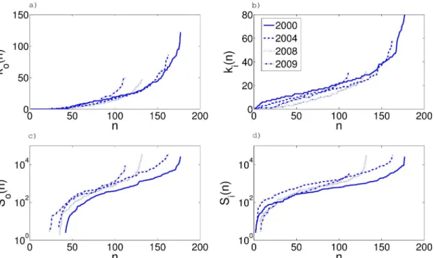
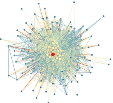
The networks we use are relatively small, ranging in size fromN= 112 toN= 177 nodes. Their out and in degree are presented inFig 1panels a) and b). Although small, these networks exhibit substantial heterogeneity in their connection patterns. This is a ubiquitous feature of all investigated financial networks. In the same figure on the panels c) and d) we present out and in network strength. Heterogeneity is again obvious in both cases. An example of one network used in simulations is presented inFig 2.
Methods
Parameters
In order to compute the cascade risk using the DebtRank methodology we impose some assumptions with respect to bank parameters. First, we define reserve requirements and then we simulate different levels of their ratios.
Assets and liabilities of subjecticonsist of five characteristic parts:total balance Bi,assets
lentto interbanking market network subjectj Aij,liabilities borrowed Ajifrom network subject
j,regulatory required balance sheet reserve Eiandregulatory required rescue fund Fi, held in the
rescue fund. Parameters found in e-MID data are interbanking market lendingAij, and
inter-banking market borrowingAji. Total assets lent to other participants of the trading network is
SL
i ¼
P
jAijand the total assets borrowed from other participants isS B
i ¼
P
jAji. We use this
two variables as out and in strength of the weighted network. We simulate balances as follows:
Bi ¼bmaxðS B
i;S
L
iÞ: ð1Þ
Fig 1. In this picture x-axis is the order of the node with respect to its value on the y-axis.The panel a) has out-degree on the y-axis, the panel b) has in-degree on the y-axis, the panel c) has out-strength on the y-axis and the panel d) has in-strength on the y-axis. The heterogeneity of all the properties is clear.
Parameterβis estimated through the publicly presented data of the money market activity compared to the total banking assets volume for the European region [35]. The typical value used in the paper isβ= 10 although we experimented with values ranging fromβ2[4, 20]. To calibrate assets and liabilities using MM data exposures, we a simple strategy of assigning the sameβto all market participants. Factorβcan be interpreted as an average of variablebi¼ Bi=maxðS
B
i;S
L
iÞcomputed separately for each institution. As long as the averageβis a good
rep-resentative of typical value of the variableβi, our estimates are economically and statistically robust.
Reserve requirementsEiare also kept in constant ratio to balance.
Ei ¼ZBi: ð2Þ
We report many different values ofη2[0,0.05] as reserve requirements vary largely depending on country and economic region [36]. Reserve requirements are regulatory attempt to force market participants to always retain some degree of resilience to market shocks and to manage the deposit multiplier for banks. In the simplified systemic liquidity crunch we assume that if the bank short term obligations become greater then its reserves—the bank would fail. Realisti-cally reserves can be very different from legally required minimum. In this case we can again assume that each institution has a reserve fractionηi=Ei/Biand that the distribution of these
fractions is well represented by their average valueη.
Fig 2. This figure shows a network of e-MID precipitants for April 2000.Thicknesses of edgesA0
ijare
recalculated from the real weightsA0
ij¼logðAij=ð0:25AminÞÞ. The core-periphery structure and weight
heterogeneity are easily observed. Size and color of the nodes correspond to out strength of the node computed with rescaled weights. Palette is color coded so that the blue links (nodes) have the lowest weight (out strength) while red carry the largest weight (out strength).
The last parameter designed in our paper is theireserve fund obligationFi(for any agent i)
affecting the market stability. We propose that each bank puts an amount
Fi ¼aEi ð3Þ
in the fund,α2[0, 1]. Therefore we use a simple strategy in which banks participate in the reserve fund proportionally to their size. Clearly different strategies in the real world are possi-ble—aflat amount tax, for instance. Other interesting choice would be to use some metric, like DebtRank, to asses banks importance to the stability of the system and to tax proportionally to that metric. We decided to use proportional tax as wefind it to be the most logical to minimize regulatory inequalities and arbitrage opportunities.
DebtRank
A previously mentioned level of defaultEiis assigned to each nodeiof the weighted directed
network. This level represents a threshold for the bank default, i.e. if the sum of noncollectable loans passes this threshold the subject fails. Theinitial level of distressψi2[0, 1] is also assigned
to each nodei.The level of distress hi(t) withhi(t)ψiis computed as an amount of losses
suf-fered by the bankiafter an iterationtof the model, divided by its own level of defaultEi. The
DebtRank starts from the initial set of nodes whoseψi>0. Loans are represented with
outgo-ing weighted links and each nodeiat iterationtincreases a level of distresshj(t) =min{1,hj(t
−1)+Wijhi(t−1)} to its neighborj. HereWij¼Aij
Ejis a fraction of distress that can pass through
the given link. Every link in the simulation can be used only once and we assign a labell2{0,1} to it. At time 0 all the links have labell= 0 and after they are used they get labell= 1 and are discarded from future consideration. The algorithm works in steps and all links have to be used before the next iteration. The last run is experienced when there are no more available links that could propagate the stress further. Finishing levels of distresshigive the impact of the
pro-cess onfinancial system.
In our simulations we start with a default of one agents, i.e.ψs= 1. We do not add additional
stress to other market subjects as this has one to one correspondence with loweringEifor the
same amount of stress. In realistic setting with additional data it would make sense to simulate additional levels of shock, if one would be interested in difference between the expected and the real systemic risk. Some other authors simulate and describe the dynamics of risk propagation process [37] and thus have to take into account subjects’correlations via mutual asset classes. We instead use the DebtRank procedure to estimate the influence of every node to the others and estimate their systemic importance. In this procedure subjects are connected only via their mutual financial dependencies. Timescale of the process is assumed small compared to the time-scale in which correlations among asset clases become important. Additionally at our timetime-scales, correlations can be represented as different initial probabilities of defaults for each node.
Rescue fund strategy
When the first bak defaults, we simulate cascading effects on other interbanking market coun-terparts. The strategy of the rescue fund operation we simulate is the following. First the initial subjectiupon request gets its fund amountFito try to prevent its default. We assume that the
initial subject always defaults. The rationale for such a decision is as follows: since every subject can ask for its own share from rescue fund if it is needed, the reserve levelEiis constant before
One of the issues for financial regulators is to minimize the moral hazard risk when bankers believe to be rescued with bail-outs solutions. In our model we introduce the opportunity to manage a default without a serious contagion, reducing the systemic risk.
When the first subject defaults all of its neighbors (lenders) receive all the money needed to stop further catastrophic cascading effects up to a value of the complete rescue fund. This is the Pigouvian idea devised in a way that no participant is subject to moral hazard of risky behavior under the protection of rescue fund, but all other market participants know that they are pro-tected with respect to risky behavior of their counter parties. If the fund is not big enough to cover all the loses the money is distributed proportionally to the sum each subject has requested.
To make this strategy viable it isa prioridesirable that:
1. the size of the rescue fund is big enough to cover the loss of financial intermediaries in the market, particularly network hubs, as a consequence of some subject default;
2. the size of the rescue fund is small enough to be easily and urgently replaced with the fresh liquidity once the fund has been used;
3. the implemented procedures of the rescue fund enable momentary usage of the fund.
Cascade risk
Here we finally present the cascade risk and the method we use to estimate it. Since we defined it a an measure of the probability of default, we address the probability of default of subjectiin a given time horizon. We split the probability of default into two components. The first compo-nent is exogenous and it is caused by an external market eventpO
i; the second component,
inde-pendent from thefirst factor, is endogenous and it caused by interbanking systemic network related riskpS
i:
pi ¼pOi þp S
i: ð4Þ
Here we operate with a simple assumption thatpO
i of every bank is small enough that we can
expect only one default in the monitored period for which we estimate systemic risk, i.e. maxðpO
iÞ N 1. We omit the“set intersection”term p O
ip
S
i assuming that it is small
com-pared to the linear approximation. This assumption does not change qualitative behavior of our taxation analysis but introduces only a slight quantitative changes. HereNis the number of subjects in the network. For the endogenous probability of defaultpS
i we can write:
pS
i ¼
X
j6¼i
QðijjÞpO
j; ð5Þ
whereQ(ijj) is conditional probability that subjectiwill default given that subjectjhas defaulted due to exogenous factors. Notice that if we would accept the possibility of simulta-neous events, the real exogenous probability would be:
pS i ¼ XN 1 s1 X
OðsÞOðN 1Þ
QðijOðsÞÞY
j2OðsÞ
pj
Y
j0=2OðsÞ ð1 p
j0Þ ð6Þ
of subjectss. Products weight the probability of occurrence of every given set of initially defaulting subjects under assumption that these events arenotcorrelated to each others.
We use the definition of the cascade riskpC
i, mentioned before and write within the
approxi-mation of only one defaulting subject:
pC
i ¼
P
j6¼iQðijjÞpOj
P
j6¼ipOj
: ð7Þ
The cascade risk of subjectiis the conditional probability that the cascade will reach the subjectinot depending on subjectjwhich initiated the cascade. Therefore we weight all the paths by probability calibrating proportionally topO
j, and we can label every cascade path by its
starting nodej. An important property of this measure is that it is invariant to scaling of exoge-nous probabilities, i.e. if we scale all the exogeexoge-nous probabilities for the same amount
gpO
j !p
0O
j )p
0C
i ¼p
C
i. This means that the values of exogenous probabilities are neutral.
We adopt the DebtRank algorithm for the simulation of default cascade, the conditional probbaility that thejdefault will affect theidefaultQ(ijj) will be coherently computed. Notice that DebtRank always provides the same solution for the same set of initial conditions, so theQ (ijj) is modelled as a binomial variable. If we further simplify our assumptions and suppose that exogenous probabilities of the default are all the same, i.e. that there is no difference among the subjects, theEq (5)reduces to
pS
i ¼DipO; ð8Þ
whereΔiis the number of times the subjectihas defaulted during the algorithm execution, and
pOis exogenous probability of default which is the same for all the subjects. In this case overall probability of default is
pi ¼ ð1þDiÞpO: ð9Þ
The cascade risk of subjectiin this case is:
pC
i ¼
Di
N 1: ð10Þ
The cascade risk of the system we define as the average cascade risk of all subjects:
pC¼
P
ipCi
N ¼
P
iDi
NðN 1Þ: ð11Þ
Eq (11)is the measure that quantifies individual exposure of the institution to risky behavior of other financial counterparts. Notice that the cascade risk does not explain anything about the number of subjects that can default or about the level of financial shock the MM will suffer in the case of default cascade. It should therefore be seen as an individual measure to explain the risk that the financial system estimates for the individual subject.
Effect on the return on investment (ROI)
significantly increased through the positive effects of the rescue fund taxation, there could also be positive effects to their debt cost along with the market acceptance of their securities, with a virtuous circle. To quantify this effect we use the following method.
Every subject records anominalreturn of investment of their assetsROIN
i and a
risk-adjustedcounterpartROIRA
i .
We classify the ROI in two categories: theROINfor assets inside the network isROIint, and the ROI for assets outside the network isROIext. We also introduceROIEwhich is the return on investment tied to the balance sheet reserve. In that case the total nominal return on invest-ment is
ROIN
i ¼
ROIintP
j6¼iAijþROI
extD
iþROI
EE
i
Bi
; ð12Þ
whereDi=Bi− ∑j6¼iAij−Eiis a total volume of assets allocated outside the money market.
Risk-adjustedROI is defined as
ROIRA
i ¼ROI
N
i ð1 piÞ pi; ð13Þ
wherepiis the bankiinvestment horizon default probability. This enables us to calculate the
effects of rescue fund on risk-adjusted return on investmentROIRA. Before the fund introduc-tion we can computeROIRAas follows:
ROIRA
i ¼ ROI
N
i ð1 p
O
i p
S
iÞ p
O
i p
S i
¼ ROIN
i 1 p
O i X j6¼i QðijjÞpO j ! pO i X j6¼i QðijjÞpO j: ð14Þ
Using the assumption that exogenous probabilities are all the same, i.e.8j: pO
j ¼pO, we
obtain:
ROIRA
i ¼ROI
N
i ð1 ð1þDiÞpOÞ ð1þDiÞpO: ð15Þ
After introducing the fund parametrized through the taxation rateαof the balance sheet reserves, default probabilities change topi(α) and systemic probabilities becomepSiðaÞ. Note
that exogenous default probabilitiespO
i andp
Odo not change as our strategy allows for every
subject to withdraw the money from the fund if needed. Now the risk-adjusted ROI becomes
ROIRA
i ðaÞ ¼ROI
N
i ðaÞ ð1 piðaÞÞ piðaÞ: ð16Þ
NominalROIN
i ðaÞalso depends onαbecause some portion of assets is allocated to the rescue
fund. We model nominal ROI with the rescue fund as:
ROIN
i ðaÞ ¼
ROIintP
j6¼iAijþROI
extD
iþROI
Eð1 aÞE
iþROI
FaE
i
Bi
: ð17Þ
Typical values of the parameters used in our simulations areROIint= 0.04,ROIext= 0.07, ROIE= 0.03,ROIF= 0.02 andpO= 0.001. We have thoroughly investigated other values of parameters, with special focus on thepO,ROIEandROIFfinding the same qualitative picture in all cases. In some scenarios we find a declining linear regime inROIRAfor the cases whenROIF
specific asset classes [35,38]. Note that in this analysis we assume total loss on the ROI after the default. Clearly, this assumption could be relaxed if needed.
Results
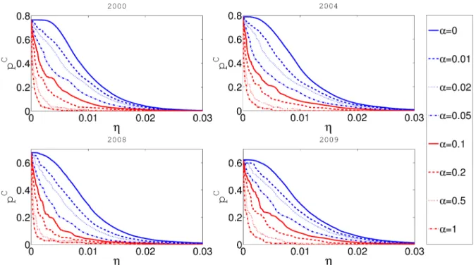
Using the methodology reported in previous sections of this paper we run a number of simula-tions to investigate the relasimula-tionships between systemic risk, risk-adjusted ROI, and the rescue fund. InFig 3we present the relationship between the level of balance sheet reserve require-mentsηand the cascade riskpC. Clearly, as the rate of reserve requirements increases, the cas-cade risk decreases. Also the cascas-cade risk is much lower if some taxation rateαis present. The effect of reserve fund is especially strong for small and most realistic values ofη. Different val-ues in different panels are a consequence of different networks used for each panel.
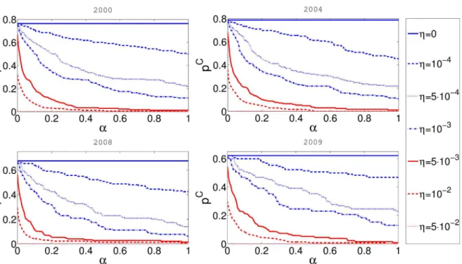
A more interesting question is how cascade risk changes with respect to taxation rateα. The results are presented inFig 4. It is obvious that the initial level of reserve requirementsηalso strongly influences the outcomes. If there are no reserves, the rescue fund will not be funded regardless of the value ofαand consequently the cascade risk does not depend onα. As reserves increase, the parameterαplays more important role. The largest ameliorating effect of the rescue fund is found for the reserve level ranging between 0.001 and 0.01. The reserves to network exposure ratio in our model is correlated with the productβη, as seen inEq (1)andEq (2). Therefore the ratio is most affected byαis roughly between 0.01 and 0.1. We believe that this effect depends on the details of the network and the chosen parameters. The sharp fall in the cascade risk for the small values ofα, points to the fact that the best strategy for the cascade risk mitigation is to combine both the reserve levels and the rescue fund.
Fig 3. In this figure x-axis representsηand y-axis represents cascade riskpC.Different panels represent the results for networks obtained from the
aggregate of some one month data for four different years. Fixed taxation rateαis constant for every curve in the plot.
It is also interesting to point out that according to our simulations, the cascade riskpCis lower for networks which were produced from the data for years 2008 and 2009, compared to networks produced from the period 2000–2004. It is possible that during the most intense period of 2007–2009 crisis banks traded with a higher level of systemic risk awareness and pro-duced a more stable network of relationships themselves.
The DebtRank algorithm is also used to define a per node systemic risk measure called DebtRank. It signals the impact of the distress of an initial node across the whole network. The DebtRank of the nodei, designated asDRi, equals the fraction of the total economic value that
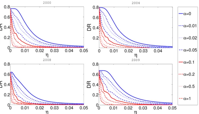
is potentially under distress after the shock at nodei. The averageDRis just the expected value of the DebtRank if initially shocked subject is chosen randomly (more details can be found in [12]). In theFig 5we present the dependence of average DebtRank with respect to different lev-els of reserve requirements. It is not surprising that the average DebtRank is decreasing with an increase of reserves, but is interesting to note that for a very modest taxation rate ofα= 0.01 the reduction of expected DR can be as high as 20%. Overall the curves on this figure look very similar to the curves inFig 3.
InFig 6we present the dependence between the taxation rateαand the DebtRankDR. The relationship is again similar to relationship between the taxation rateαand cascade riskp pre-sented inFig 4and the conclusions are similar. Again, it is clear that the reserve level and taxa-tion rate better work together to reduce the DebtRank of the system.
Aforementioned results indicate that a combination of the reserves and the taxation rate for rescue fund can greatly stabilize the system and reduce its systemic risk. As stated before, the proposed taxation strategy is devised so that it should not reduce the market liquidity, that it should be easy to implement and that it should not increase moral hazard in the system. In order to corroborate attractiveness of the proposed taxation scheme, we also compute the risk adjusted return on investments of the market players.
Fig 4. In this figure on the x-axis representsαand y-axis represents cascade riskpC.Different panels represent the results for networks obtained from
the aggregate of some one month data for four different years. Balance sheet reserve requirement rateηis constant for every curve in the plot.
Fig 5. In this figure x-axis representsηand y-axis represents systemic DebtRankDR.Different panels represent the results for networks obtained from the aggregate of some one month data for four different years. Fixed taxation rateαis constant for every curve in the plot.
doi:10.1371/journal.pone.0114928.g005
Fig 6. In this figure x-axis representsαand y-axis represents systemic DebtRankDR.Different panels represent the results for networks obtained from the aggregate of some one month data for four different years. Balance sheet reserve requirement rateηis constant for every curve in the plot.
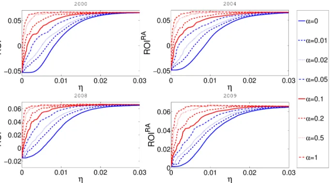
InFig 7we show the dependence betweenROIRAand the reserve levelη. Interestingly, we find a function as monotonically increasing despite the effect thatηhas on a nominal ROI. This feature is a consequence of chosen parameters becauseEiBiand the negative influence
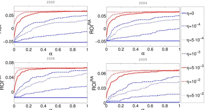
of the reserve on nominal ROI is small compared to its nonlinear influence on cascade risk. One could argue that this relation is in fact true as in reality financial institutions often hold more reserves then minimally required by imposed reserve requirements. TheFig 8shows that the influence of taxation onROIRAis not only strong but also beneficial for banks value.
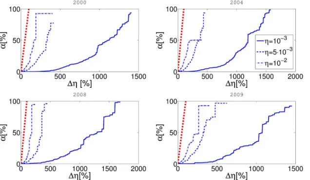
Finally inFig 9we present iso-curves for the cascade risk. Iso-curves are obtained in the fol-lowing way: First, a base reserve requirementsη0is chosen. Then we compute cascade risk for
each increase in reserve requirementsZ Z0Z0 andfindαwhich would producethe samevalue of
cascade risk,if there was no increase in reserve requirements(η=η0), but only in the taxation for the rescue fund. It is clear that for all the chosen parameters, imposing a tax ofα= 1% is much better than increasingηfor 1%. This is afinal proof that in our model, in order to reduce systemic risk, introducing a rescue fund and taxing the reserves is more effective than increas-ing reserve or capital requirements. However, in the real world, the level of reserves impacts the probability of defaultpO[39]. This is a feature we did not model in our approach, but [39] and [40] points to strong negative effects of reserve requirements increase on the liquidity of the market. Since the rescue fund should not have such adverse effects we conclude that it is, at least, a viable idea to be tested by the regulators concerned with systemic risk.
Discussion
Our model demonstrates that the cascade risk, as defined in this paper, is greatly reduced by even a small taxation for saving fund. The parameters used in simulation are artificial and
Fig 7. In this figure x-axis representsηand y-axis represents risk adjusted return on investmentROIRA.Different panels represent the results for networks obtained from the aggregate of some one month data for four different years. Fixed taxation rateαis constant for every curve in the plot.
there is a question of how well the DebtRank maps to the real world event of the default cas-cade. Nevertheless we made a case for simple proposed taxation strategy, as it is clearly more efficient in reduction of the cascade risk. Our research supports the following idea: If regulators aim at minimizing the systemic risk or more narrowly the cascade risk, the taxation for the fund is better on the performance level. Furthermore, although our implementation would require some modifications of the balance sheets, we argue that it is the cheapest of all pro-posed methods for the following reasons. Firstly, this allows to reduce the asymmetric impact of capital add-ons required to Global Systemically important financial institutions (G-SIFIs) introduced within the Basel III framework, which could corrupt the leveling the playing field principle. Secondly, it could help to design the reform for the super-national reform for safety nets, and the insurance deposit above all.
We have shown also that a very modest taxation can reduce the cascade risk so much that the risk adjusted ROI of individual subjects in a money market can greatly increase, thus mak-ing their coupons more profitable and thus possibly makmak-ing them more responsive to pre-sented idea. We believe that the Pigouvian nature of our tax and rescue fund would not increase moral hazard of individual subjects thus not affecting much the individual parameters, such as the individual probability of default.
With the introduction of the Pigouvian tax, the simulated contagion effect due to some bankrupt agents decreases to become“sustainable”. The proposal sizes the rescue fund (i) big enough to cover the loss of most of the individual institutions in the market as a consequence of some failures; (ii) small enough to be easily and urgently replaced with the fresh liquidity
Fig 8. In this figure x-axis representsαand y-axis represents the risk adjusted return on investmentROIRA.Different panels represent the results for
networks obtained from the aggregate of some one month data for four different years. Balance sheet reserve requirement rateηis constant for every curve in the plot.
once the fund has been used. In order to manage the stability inefficiency trade off of financial firms, we paid a close attention to banks’profitability measuread with the return on investment (ROI) as well, because the regulatory measure has to both be efficient, and influence the market profitability as little as possible. A considerable portion of moral hazard is reduced by construc-tion as the rescue fund assets do not cover initial troubled subject, but its counter parties. Accordingly with the profitability constraint, the impact of the reserve fund is strong with small and realistic values of the taxation rate. In order to minimize and manage the systemic risk, based on our analysis the tax could range from 2 to 4bps of banks’balance. To avoid any additional moral hazard behaviour, policy makers should better calibrate the tax taking into account all the money market trades to map more precisely the bank network topology and fix-ing a time period fixed tax.
In conclusion, the debate on rescue policies which ranges from raising of capital require-ments to implementation of money market taxation on transactions is expected to enhance a fiscal proposal coherently with the economic theoretical background and the banking role played both in the monetary and credit markets.
Acknowledgments
Both VZ and HA worked on the technical details of the paper. Survey of the literature was done by HA and GG and a mechanism for taxation was proposed by HA. All the authors con-tributed to writing of the paper. Authors acknowledge support from EU FP7 FET OPEN
Fig 9. In this figure x-axis represents percentage of change ofηand y-axis representsα.Curves represent the points at which the systemic probability
of default takes the same value in the case(i)when no fund is present, i.e.α= 0 and the system is stabilized through increase of reserve requirements byΔη and(ii)when there is no change in reserve requirements, but the stabilization of the system is implemented through the rescue fund. Three starting levels of reserve requirements are presented through three different curves. The red fat dashed line represents hypothetical case in which the influence of reserve requirements increase by percentagexwould be exactly the same as if the proposed taxation was implemented with the same ratex. Different panels represent the results for networks obtained from the aggregate of some one month data for four different years.
project FOC (Forecasting financial crises, grant no. 255987). VZ also acknowledges support from EU FP7 FET project MULTIPLEX (Foundational Research on MULTIlevel comPLEX networks and systems, grant No. 317532). GG also acknowledges support from EU Framework Program SSH.2010.1.2-1 (FESSUD) and SDA Bocconi School of Management for data acquisi-tion. Authors also want to express their gratitude to Stefano Battiston, Giulia Iori and Hrvoje Stefancic on fruitful comments of the paper.
Author Contributions
Conceived and designed the experiments: HA VZ GG. Performed the experiments: HA VZ. Analyzed the data: HA VZ. Contributed reagents/materials/analysis tools: HA. Wrote the paper: HA VZ GG.
References
1. Angelini P, Maresca G, Russo D (1996) Systemic risk in the netting system. Journal of Banking & Finance 20: 853–868. doi:10.1016/0378-4266(95)00029-1
2. Eisenberg L, Noe TH (2001) Systemic risk in financial systems. Management Science 47: 236–249. doi:10.1287/mnsc.47.2.236.9835
3. Iori G, Jafarey S, Padilla FG (2006) Systemic risk on the interbank market. Journal of Economic Behav-ior & Organization 61: 525–542. doi:10.1016/j.jebo.2004.07.018
4. May RM, Levin SA, Sugihara G (2008) Complex systems: Ecology for bankers. Nature 451: 893–895. doi:10.1038/451893aPMID:18288170
5. Haldane AG, May RM (2011) Systemic risk in banking ecosystems. Nature 469: 351–355. doi:10. 1038/nature09659PMID:21248842
6. Cont R, Moussa A, Santos E (2011) Network structure and systemic risk in banking systems. Edson Bastos e, Network Structure and Systemic Risk in Banking Systems (December 1, 2010).
7. Whelan K (2009) Containing systemic risk. Technical report, European Parliament, Committee on Eco-nomic and Monetary Affairs, Research Department.
8. Upper C (2011) Simulation methods to assess the danger of contagion in interbank markets. Journal of Financial Stability 7: 111–125. doi:10.1016/j.jfs.2010.12.001
9. Freixas X, Parigi BM, Rochet JC (2000) Systemic risk, interbank relations, and liquidity provision by the central bank. Journal of money, credit and banking: 611–638. doi:10.2307/2601198
10. Iori G, Jafarey S (2001) Criticality in a model of banking crises. Physica A: Statistical Mechanics and its Applications 299: 205–212. doi:10.1016/S0378-4371(01)00297-7
11. Boss M, Elsinger H, Summer M, Thurner S (2004) Network topology of the interbank market. Quantita-tive Finance 4: 677–684. doi:10.1080/14697680400020325
12. Battiston S, Puliga M, Kaushik R, Tasca P, Caldarelli G (2012) Debtrank: Too central to fail? financial networks, the fed and systemic risk. Scientific reports 2.
13. Acharya V, Pedersen L, Philippon T, Richardson M (2012) Measuring systemic risk. CEPR Discussion Paper No DP8824, CEPR Discussion Papers.
14. Brownlees CT, Engle R (2010) Volatility, correlation and tails for systemic risk measurement. New York University, mimeo.
15. Adrian T, Brunnermeier MK (2011) Covar. Technical report, National Bureau of Economic Research.
16. Hu D, Zhao JL, Hua Z, Wong MCS (2012) Network-based modeling and analysis of systemic risk in banking systems. MIS Q 36: 1269–1291.
17. Drehmann M, Tarashev N (2013) Measuring the systemic importance of interconnected banks. Journal of Financial Intermediation 22: 586–607. doi:10.1016/j.jfi.2013.08.001
18. D’Agostino G, Scala A, ZlatićV, Caldarelli G (2012) Robustness and assortativity for diffusion-like pro-cesses in scale-free networks. EPL (Europhysics Letters) 97: 68006. doi:10.1209/0295-5075/97/ 68006
19. Battiston S, Delli Gatti D, Gallegati M, Greenwald B, Stiglitz JE (2012) Liaisons dangereuses: Increas-ing connectivity, risk sharIncreas-ing, and systemic risk. Journal of Economic Dynamics and Control 36: 1121–
20. Battiston S, Gatti DD, Gallegati M, Greenwald B, Stiglitz JE (2012) Default cascades: When does risk diversification increase stability? Journal of Financial Stability 8: 138–149. doi:10.1016/j.jfs.2012.01. 002
21. Horváth BL, Wagner W (2013) The disturbing interaction between countercyclical capital requirements and systemic risk. Available at SSRN.
22. Gauthier C, Lehar A, Souissi M (2012) Macroprudential capital requirements and systemic risk. journal of Financial Intermediation 21: 594–618. doi:10.1016/j.jfi.2012.01.005
23. Hart O, Zingales L (2011) A new capital regulation for large financial institutions. American Law and Economics Review 13: 453–490. doi:10.1093/aler/ahr001
24. Hellwig M (2010) Capital regulation after the crisis: business as usual? Technical report, Preprints of the Max Planck Institute for Research on Collective Goods.
25. Poledna S, Thurner S (2014) Elimination of systemic risk in financial networks by means of a systemic risk transaction tax. arXiv 14018026.
26. Darvas Z, Weizsäcker J (2011) Financial transaction tax: small is beautiful. Society and Economy 33: 449–473. doi:10.1556/SocEc.33.2011.3.2
27. Schäfer D, Schulmeister S, Vella J, Masciandaro D, Passarelli F, Buckley RP (2012) The financial transaction tax—boon or bane? Intereconomics 47: 76–103. doi:10.1007/s10272-012-0409-8
28. Iori G, De Masi G, Precup OV, Gabbi G, Caldarelli G (2008) A network analysis of the italian overnight money market. Journal of Economic Dynamics and Control 32: 259–278. doi:10.1016/j.jedc.2007.01. 032
29. Finger K, Fricke D, Lux T (2012) Network analysis of the e-mid overnight money market: The informa-tional value of different aggregation levels for intrinsic dynamic processes. Technical report, Kiel Work-ing Paper.
30. Raddant M (2013) Structure in the italian overnight loan market. Journal of International Money and Finance.
31. Hatzopoulos V, Iori G, Mantegna RN, Micciche S, Tumminello M (2013) Quantifying preferential trading in the e-mid interbank market. Technical report.
32. Hojman DA, Szeidl A (2008) Core and periphery in networks. Journal of Economic Theory 139: 295–
309. doi:10.1016/j.jet.2007.07.007
33. Fricke D, Lux T (2012) Corperiphery structure in the overnight money market: Evidence from the e-mid trading platform. Technical report, Kiel Working Papers.
34. Zlatic V, Bianconi G, Díaz-Guilera A, Garlaschelli D, Rao F, Caldarelli G (2009) On the rich-club effect in dense and weighted networks. The European Physical Journal B 67: 271–275. doi:10.1140/epjb/ e2009-00007-9
35. Schlüter T, Hartmann-Wendels T, Busch R, Sievers S (2012) Determinants of the interest rate pass-through of banks—evidence from german loan products. Technical report, Deutsche Bundesbank.
36. O’Brien YYC (2007) Reserve requirement systems in oecd countries. FEDS Working Paper.
37. Xuqing H, Irena V, Shlomo H, Eugene SH (2013) Cascading failures in bi-partite graphs: Model for sys-temic risk propagation. Sci Rep 3.
38. Iakova D, Wagner N (2001) Financial Sector Evolution in the Central European Economies:Challenges in Supporting Macroeconomic Stability and Sustainable Growth. International Monetary Fund. URL http://books.google.hr/books?id = tcuNgEuiDeIC
39. Agur I (2010) Capital requirements and credit rationing. Technical report, Netherlands Central Bank, Research Department.