SRef-ID: 1432-0576/ag/2004-22-3155 © European Geosciences Union 2004
Annales
Geophysicae
Latitudinal extension of low-latitude scintillations measured with a
network of GPS receivers
C. E. Valladares1, J. Villalobos2, R. Sheehan1, and M. P. Hagan1
1Institute for Scientific Research, Boston College, Newton Center, Massachusetts, USA 2Department of Physics , Universidad Nacional de Colombia, Bogota, Colombia
Received: 1 December 2003 – Revised: 8 April 2004 – Accepted: 12 May 2004 – Published: 23 September 2004 Part of Special Issue “Equatorial and low latitude aeronomy”
Abstract.A latitudinal-distributed network of GPS receivers has been operating within Colombia, Peru and Chile with sufficient latitudinal span to measure the absolute total elec-tron content (TEC) at both crests of the equatorial anomaly. The network also provides the latitudinal extension of GPS scintillations and TEC depletions. The GPS-based informa-tion has been supplemented with density profiles collected with the Jicamarca digisonde and JULIA power maps to in-vestigate the background conditions of the nighttime iono-sphere that prevail during the formation and the persistence of plasma depletions. This paper presents case-study events in which the latitudinal extension of GPS scintillations, the maximum latitude of TEC depletion detections, and the alti-tude extension of radar plumes are correlated with the loca-tion and extension of the equatorial anomaly. Then it shows the combined statistics of GPS scintillations, TEC deple-tions, TEC latitudinal profiles, and bottomside density pro-files collected between September 2001 and June 2002. It is demonstrated that multiple sights of TEC depletions from different stations can be used to estimate the drift of the back-ground plasma, the tilt of the plasma plumes, and in some cases even the approximate time and location of the tion onset. This study corroborates the fact that TEC deple-tions and radar plumes coincide with intense levels of GPS scintillations. Bottomside radar traces do not seem to be as-sociated with GPS scintillations. It is demonstrated that scin-tillations/depletions can occur when the TEC latitude profiles are symmetric, asymmetric or highly asymmetric; this is dur-ing the absence of one crest. Comparison of the location of the northern crest of the equatorial anomaly and the max-imum latitude of scintillations reveals that for 90% of the days, scintillations are confined within the boundaries of the 50% decay limit of the anomaly crests. The crests of the anomaly are the regions where the most intense GPS scin-tillations and the deepest TEC depletions are encountered. In accord with early results, we observe that GPS
scintilla-Correspondence to:C. E. Valladares
tions/TEC depletions mainly occur when the altitude of the magnetic equator F-region is above 500 km. Nevertheless, in many instances GPS scintillations and TEC depletions are observed to exist when the F-layer is well below 500 km or to persist when the F-layer undergoes its typical nighttime de-scent. Close inspection of the TEC profiles during scintilla-tions/depletions events that occur when the equatorial F-layer peak is below 500 km altitude reveals that on these occasions the ratio of the crest-to-equator TEC is above 2, and the crests are displaced 10◦or more from the magnetic equator. When the equatorial F-layer is above 500 km, neither of the two re-quirements is needed, as the flux tube seems to be inherently unstable. We discuss these findings in terms of the Rayleigh-Taylor instability (RTI) mechanism for flux-tube integrated quantities. We advance the idea that the seeming control that the reverse fountain effect exerts on inhibiting or suppressing GPS scintillations may be related to the redistribution of the density and plasma transport from the crests of the anomaly toward the equatorial region and then to much lower alti-tudes, and the simultaneous decrease of the F-region altitude. These two effects originate a decrease in the crest/trough ra-tio and a reducra-tion of the crests separara-tion, making the whole flux tube more stable to the RTI. The correspondence be-tween crest separation, altitude of the equatorial F-region, the onset of depletions, and the altitude (latitude) extension of plumes (GPS scintillations) can be used to track the fate of the density structures.
Key words. Ionosphere (Equatorial ionsphere; ionospheric irregularities; modeling and forecasting)
1 Introduction
of kilometers down to sub-meter sizes. A basic understand-ing of ESF has been obtained due to insights from Jicamarca measurements (Woodman and LaHoz, 1976), satellite in-situ observations (McClure et al., 1977), and numerical model-ing of the Rayleigh-Taylor instability (Ossakov et al., 1979; Zalesak and Ossakov, 1980). Woodman and LaHoz (1976), almost 3 decades ago, presented two-dimensional maps of coherent echoes to indicate that plume-like structures extend for hundreds of kilometers in altitude, connecting the unsta-ble bottomside F-region with the spread F on the staunsta-ble top-side. The radar maps provided strong evidence for a plasma density depletion convecting upward, following a Raleigh-Taylor Instability (RTI) mechanism. McClure et al. (1977) used plasma composition measured by the RPA on board the AE-C satellite to demonstrate that the plasma biteouts or depletions, seen in the nighttime equatorial F-region, some-times contained molecular ions. This fact implied that the plasma depletions had recently moved from the low bottom-side. Numerical calculations of the RTI conducted by Ott (1978) provided the rising velocity of the plasma bubbles in the collisional and inertial regimes, well in accord with ex-perimental values. Computer simulations of the nonlinear collisional RTI carried out by Ossakov et al. (1979) demon-strated the production of topside irregularities by the rising bubbles and the dependence of the instability growth rate on the altitude of the F-layer and the gradient scale-size. Zalesak et al. (1982) incorporated the zonal neutral wind and an underlying E-region conductivity in their simulations and were able to demonstrate that these processes produce a slow-down effect in the evolution of ESF. Satyanarayana et al. (1984) investigated the effect of a velocity shear in the RTI that tends to stabilize the small-scale irregularities and excite long wavelength modes. Zargham and Seyler (1987) used boundary conditions proper for the nighttime F-layer to show the inherently anisotropic state of the generalized RTI. According to their numerical results, they postulated that a predominant km-scale wavelength develops in the zonal di-rection for an eastward-directed effective electric field, and shocklike structures are formed along the vertical direction.
It is well accepted that near sunset, the dynamics of the equatorial ionosphere are dominated by the pre-reversal en-hancement (PRE) (Woodman, 1970) of the vertical drift, and that the variability of this process may dictate the onset or not of ESF (Basu et al., 1996; Fejer et al., 1999; Hysell and Burcham, 1998). The rapid decay of the E-region conduc-tivity produces polarization electric fields that vary greatly in local time and latitude. The PRE is originated by a response of the electric fields to maintain a curl-free nature near sun-set (Eccles, 1998), but is modified, up to some extent, by the divergence of zonal Hall currents in the off-equatorial E-region (Farley et al., 1986) and/or the zonal Cowling con-ductivity gradients in the electrojet (Haerendel and Eccles, 1992). The maximum value of the PRE has been asso-ciated with the generation and evolution of ESF (Fejer et al., 1999). These authors found that during solar minimum conditions a PRE larger than 15–20 m/s implied the occur-rence of radar plumes extending to the topside. During
so-lar maximum conditions, (>200) a PRE of 40–45 m/s was required for the generation of ESF. When the PRE is fully developed, the Appleton anomaly is seen to re-intensify af-ter sunset, making the crests more prominent and displaced even further away (15◦-20◦) from the magnetic equator. This
close relationship between vertical drifts, the location of the crests of the anomaly, and ESF has been noted by several researchers (Whalen, 2001; Valladares et al., 2001). Oth-ers have used the amplitude of the equatorial anomaly to de-fine precursors of the occurrence of ESF (Raghavarao et al., 1988; Sridharan et al., 1994). Whalen (2001) used bottom-side densities collected by a network of sounders that oper-ated in September 1958 to demonstrate that strong bottom-side spread F (BSSF) and bubbles occurred when the crest density exceeded 3.5×106cm−3, and the anomaly peak was
located poleward of 15.4◦dip latitude. Weaker BSSF was
ob-served when the crest of the anomaly was smaller and closer to the equator. No BSSF was detected when the peak density was below 3.5×106cm−3 or if the crest was non-existent.
Valladares et al. (2001) used TEC values measured with 6 GPS receivers forming a latitudinal chain, to show that dur-ing the equinoxes a crest-to-trough ratio equal to 2 or larger always implied the onset of UHF scintillations and the pres-ence of radar plumes in the JULIA maps.
In addition to the vertical drift and the altitude of the F-layer, a downward vertical wind makes the F-region un-stable to the initiation of the RTI. The meridional wind can also influence the onset of irregularities, by making the F-region more stable and inhibiting ESF. Maruyama and Matura (1984) and Maruyama (1988) indicated that a transe-quatorial wind could depress the F-layer in the lee side hemi-sphere, changing the field-integrated Pedersen conductiv-ity and, consequently, suppressing the growth of the RTI. Mendillo et al. (1992) presented measurements from the Al-tair incoherent scatter radar and all-sky optical images pro-viding evidence that a southward wind was somewhat re-sponsible for lowering the density contours and making the whole flux tube more stable to the onset of the RTI. More recently, Mendillo et al. (2001) have re-examined the impor-tance of the meridional winds in suppressing ESF during a campaign in South America. These researchers concluded that during the eight days of the campaign in September 1998, the meridional wind did not influence the onset of ESF in the pre-midnight hours. However, Devasia et al. (2002) have presented evidence that suggests that whenh′F is below 300 km, ESF may occur only for a thermospheric meridional wind directed equatorward and less than 60 m/s.
This paper shows TEC values measured by a network of ten GPS receivers during ten months, spanning September 2001 and June 2002. We present GPS scintillations measured by three of these receivers in an effort to assess the latitudinal (and apex altitude) extension of the plasma bubbles. We also used information of TEC depletions, and range-time maps of coherent echoes collected with the JULIA radar, to indicate the spatial location of plasma biteouts and to infer that the GPS scintillations, in fact, correspond to plasma bubbles or depletions in the equatorial F-region. We also investigate the background conditions of the equatorial ionosphere, by pro-viding the location of the crests and the trough. Three events are analyzed in detail and the statistics of the first 10 months of operations at Bogota are introduced to demonstrate that in most cases the plasma bubbles extend up to the poleward edges of the anomaly. Finally, we use measurements con-ducted with the Jicamarca digisonde to corroborate the re-lationship between the appearance of GPS scintillations and the altitude of the F-region.
2 Instrumentation
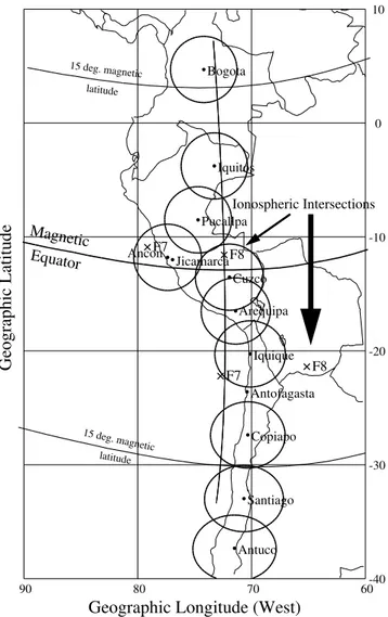
TEC measurements were gathered using 10 GPS receivers located near the west coast of South America, and span-ning in latitude between 9◦N and 40◦S. Their fields-of-view are indicated in Fig. 1, using circles extending 45◦in eleva-tion. Five of these receivers are managed by BC. These re-ceivers have been implemented with specially-designed soft-ware that makes real-time calculations of the amplitude scin-tillations. Four of the sites (Bogota, Iquitos, Pucallpa and Cuzco) are equipped with CRS1000 Leica receivers running at 10 Hz. The last of the five sites (Ancon) possesses two GPS receivers, a Novatel that records GPS signals at 50 Hz, and an Ashtech receiver dedicated to measure TEC values. Figure 1 also displays the geographic location of the mag-netic equator and the 15◦magnetic latitude line. Note that the Bogota and Santiago stations are practically conjugate from the magnetic equator. These two receivers are able to measure, quite frequently, the TEC value in the northern and southern crests of the anomaly. Other systems, such as the UHF (∼250 MHz) and L-band scintillation receivers, have operated at Ancon and Antofagasta since 1994 and 1996, re-spectively. These systems measure the S4 index, the spectra of the amplitude scintillation, and the zonal drift of the ir-regularities (Valladares et al., 1996), using the space-antenna technique. The ionospheric penetration points correspond-ing to the UHF systems are shown with the large crosses, and labeled F7 and F8. These points are the 350-km alti-tude intersection of the lines-of-sight directed to 2 geosyn-chronous satellites parked at the 100◦W and 23◦W meridi-ans. A ground projection of the magnetic field line passing above the Ancon F8 ionospheric intersection has been traced to indicate that this point and the Antofagasta F7 intersec-tion point are almost aligned along the same field line. The apex altitude of this field line is at 1200 km over the magnetic equator and is displayed ending in the F-region (350 km) near
Figure 1.
90 80 70 60-40
-30 -20 -10 0 10
F7
F8
F7 F8
Geographic Longitude (West)
Geographic Latitude
Ionospheric Intersections
Magnetic
Equator
15 deg. magnetic latitude 15 deg. magnetic
latitude
Ancon
Jicamarca Bogota
Santiago Arequipa
Iquique
Antofagasta
Copiapo
Antuco Iquitos
Pucallpa
Cuzco
Fig. 1. Geographic locations of several GPS receivers operating
near the west coast of South America. The stations at Ancon, Cuzco, Pucallpa, Iquitos and Bogota form the North Andes Project (NAP) network. The stations at Iquique, Copiapo and Antuco are part of the South Andes Project (SAP) network. The stations at Arequipa and Santiago correspond to the IGS network of receivers. The locations of the Jicamarca radar and the sub-ionospheric inter-sections of the lines-of-sight from the Ancon and Antofagasta UHF receivers to the F7 and F8 satellites are also included. The line crossing the F8 intersection point shows the ground projection of a field line with apex height equal to 1200 km that ends at 350 km altitude.
Bogota in the north and close to Santiago in the south. This paper also presents altitude-time maps of coherent echoes collected with the JULIA radar. A comprehensive descrip-tion of this system can be found in the publicadescrip-tion by Hysell and Burcham (1998).
3 TEC depletions
(a)
10 20 30 40 50 60 70
80 September 07, 2001
TEC Units
Bogota site prn = 01
19 20 21 22
S4 0.25
0.50
(b)
20 30 40 50 60 70
80 September 07, 2001
TEC Units
Iquitos site prn = 31
19 20 21 22
S4 0.25
0.50
(c)
19 20 21 22
10 20 30 40
50 September 07, 2001
TEC Units
Ancon site prn = 11
(d)
20 30 40 50
60 September 07, 2001
TEC Units
Cuzco site prn = 11
19 20 21 22
S4 0.25
0.50
(e)
19 20 21 22
10 20 30 40 50
60 September 07, 2001
TEC Units
Arequipa site prn = 01
(f)
19 20 21 22
30 40 50 60 70 80
90 September 07, 2001
TEC Units
Copiapo site prn = 11
(g)
19 20 21 22
30 40 50 60 70 80
90 September 07, 2001
TEC Units
Santiago site prn = 01
Local Time
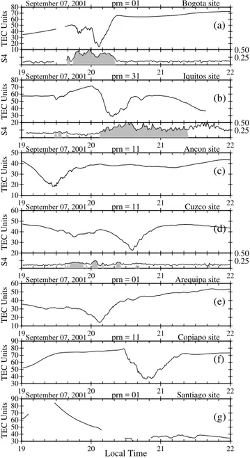
Fig. 2.Values of absolute TEC measured at several sites using
sig-nals from 3 GPS satellites. In all of these passes TEC depletions are evident, sometimes exceeding 50 TEC units (1016el/m2). The additional sub-panel plotted below the Bogota, Iquitos and Cuzco TEC data corresponds to the S4 GPS scintillation index. Note that the minimum at Arequipa coincides with the minimum at Bogota,
which is located∼200 km to the west. As the bubbles move
to-ward the east, TEC depletions should be observed at Bogota tens of min ahead of Arequipa. This discrepancy can be explained by the westward tilt of the plumes. See text for details.
the depletion. A TEC depletion originates when one or more plasma bubblesE×Bdrift across the satellite ray path. The general morphology of TEC depletions and their association with strong levels of VHF scintillations were described by DasGupta et al. (1983). More recently, Weber et al. (1996) have showed that there exists a strong correlation between TEC depletions and airglow 630.0 nm depletions,
endors-ing the view that TEC depletions are a manifestation of the equatorial plasma depletions (also called bubbles). In this section, we use the information about TEC depletions gath-ered by a network of GPS receivers to infer the presence and the north-south extension of plasma bubbles. Neverthe-less, we are aware that other non-bubble-related processes could produce quick reductions in the TEC value, and lead to a mistaken identification of the TEC depletions. Processes such as the nighttime decay of the F-layer and the density re-distribution caused by the fountain effect also lessen the TEC value. However, these two types of processes result in shallow TEC slopes and an absence of the recovery seg-ment. We have excluded these cases from our statistics of TEC depletions. Different than previous studies, the TEC depletions presented here were sequentially detected by sev-eral of the 10 receivers located at different longitudes, pro-viding a glimpse of the temporal evolution of the plasma de-pletions. Due to the relatively slow east-west motion of the GPS satellites, it is fair to say that the plasma depletions are traversing a quasi-stationary receiver-satellite link. We also note that the temporal duration of the passage of TEC deple-tion is a funcdeple-tion of the bubble width and the satellite eleva-tion. A pass near zenith will provide a TEC depletion width almost equal to the true bubble cross section. As the line-of-sight elevation becomes lower the TEC depletion will appear much wider. We also note that the depth of the TEC deple-tion is more likely to be a funcdeple-tion of the local F-region peak density, the value of the underlying equatorial bottomside, and the magnetic latitude of the observation point. Assum-ing that the density remains constant along the depleted flux tube (Hanson and Bamgboye, 1984), there may exist a more pronounced depletion at the crest of the anomaly than at the magnetic equator.
Figure 2 shows TEC depletions measured at several sites, using signals from three different GPS satellites. On this day, TEC depletions were observed at all stations except Antuco. In addition, the receiver at Santiago suffered a loss of signals caused by the strong fading which was likely associated with TEC depletions. Figure 2a shows the passage of a TEC de-pletion, 35 TEC units (1016el/m2)in depth, detected by the receiver at Bogota between 20:00 and 20:20 LT. Below the TEC curve, we display the S4 index that is calculated on-line using the signal received from each of GPS satellites. The gray shading indicates the times when the S4 index is above the noise level and the satellite elevation is above 20◦. The
depletions between Ancon and Cuzco (65 min) that are sepa-rated by 550 km in the magnetic east-west direction, and cal-culated a 140 m/s average zonal drift. Scintillations at Cuzco (Fig. 2d) were less intense, due to a smaller density that com-monly prevails near the magnetic equator when the anomaly is fully developed. At Arequipa, the lowest value within the TEC depletion was observed at 20:08 UT. This is the same time that the minimum TEC was detected in Bogota (Fig. 2a), which is located 225 km west and several hundred kilome-ters north of Arequipa. This apparent discrepancy can be explained if we allow the bubbles to tilt westward at altitudes above the F-region peak (Woodman and LaHoz, 1976). The westward tilt will make the part of the TEC depletions that extends to higher latitudes to appear at slightly later times in a way similar to the plasma plumes seen with coherent radars. The Copiapo receiver (Fig. 2f) detected a 30 TEC units de-pletion spanning between 20:30 and 21:10 LT. As mentioned before, the receiver at Santiago was strongly affected by deep fades, likely associated with the turbulence within the deple-tions, suffered several data dropouts, and recorded only mi-nor TEC disturbances.
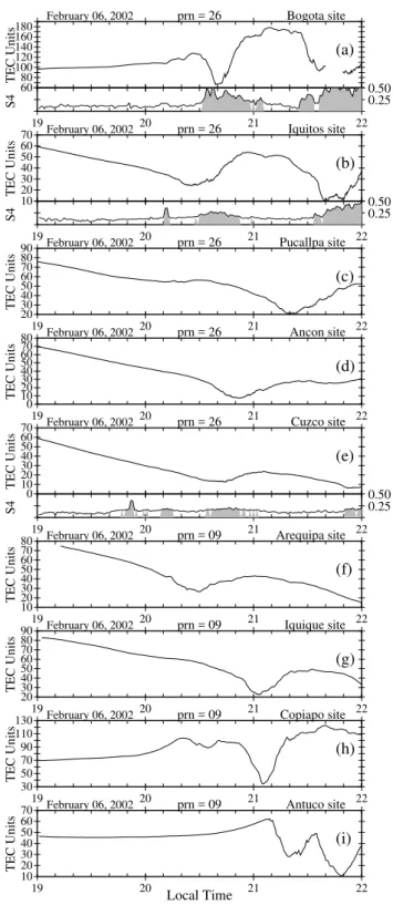
Figure 3 displays the passage of two deep TEC deple-tions, which were observed by several of the receivers on 6 February 2002. Figures 3a–3i display TEC values collected from signals transmitted only by 2 GPS satellites. The sub-ionospheric intersections between satellite 26 and the sites at Bogota, Iquitos, Pucallpa, Ancon and Cuzco varied in a south to north fashion, following a direction almost aligned with the local field line. The ionospheric penetration point from GPS satellite 09 passed south of Arequipa, Iquique, Copiapo, and Antuco, moving from west to east. Figure 3a shows that GPS scintillations at Bogota are equally intense on both sides of the depletion. However, at lower magnetic latitudes stations such as Iquitos and Cuzco (Figs. 3b and 3e), we observed that the west wall of the depletion pos-sesses larger S4 values than the east side. Similar to Fig. 2 the plasma bubbles drift through the stations’ fields-of-view at slightly different times. This means that a plasma bubble aligned with the B field and with no tilt in altitude will se-quentially go through Ancon, Pucallpa, Bogota, Iquitos and Cuzco. If the bubble is tilted in altitude, as most of them are, then the station located further poleward, Bogota, may detect the TEC depletion after it has passed over a more equator-ward station located further to the east, as Iquitos. This is the most likely physical scenario that can explain the TEC data recorded on 6 February 2002, as the first TEC depletion was seen at Iquitos at 20:25 LT, then at Bogota at 20:40 LT, and later at Cuzco∼20:45 LT. In addition, traces of the temporal variability of the sub-ionospheric intersections from different stations but toward the same GPS satellite display almost par-allel curves separated by the distance between the stations. It is quite significant that the Ancon and Pucallpa stations did not observe any TEC depletion before 20:25 LT. The impli-cation of the last statement is that the depletion, seen at Iq-uitos at 20:25 LT, appeared in a location between Pucallpa and Iquitos, near the 74◦W meridian and was triggered ap-proximately at 20:20 LT. A different TEC depletion was seen
Figure 3. (a) 60 80 100 120 140 160
180 February 06, 2002
TEC Units
Bogota site prn = 26
19 20 21 22
S4 0.25 0.50 (b) 10 20 30 40 50 60
70 February 06, 2002
TEC Units
Iquitos site prn = 26
19 20 21 22
S4 0.25
0.50
(c)
19 20 21 22
20 30 40 50 60 70 80
90 February 06, 2002
TEC Units
Pucallpa site prn = 26
(d)
19 20 21 22
0 10 20 30 40 50 60 70
80 February 06, 2002
TEC Units
Ancon site prn = 26
(e) 0 10 20 30 40 50 60
70 February 06, 2002
TEC Units
Cuzco site prn = 26
19 20 21 22
S4 0.25
0.50
(f)
19 20 21 22
10 20 30 40 50 60 70
80 February 06, 2002
TEC Units
Arequipa site prn = 09
(g)
19 20 21 22
20 30 40 50 60 70 80
90 February 06, 2002
TEC Units
Iquique site prn = 09
(h)
19 20 21 22
30 50 70 90 110
130 February 06, 2002
TEC Units
Copiapo site prn = 09
(i)
19 20 21 22
10 20 30 40 50 60
70 February 06, 2002
TEC Units
Antuco site prn = 09
Local Time
Fig. 3. Same as Fig. 2, but for 6 February 2002. Plasma bubbles
drift through the stations fields-of-view at slightly different times. One TEC depletion was seen first at Iquitos at 20:25 LT, then at
20:40 LT at Bogota, and later at Cuzco∼20:45 LT. Ancon and
Pu-callpa did not observe the TEC depletion, suggesting that the deple-tion developed in a locadeple-tion between Pucallpa and Iquitos, near the
19 20 21 22 23 24 1 0
100 200 300 400 500 600 700 800 900
30 dB S/N
-10 dB
Height (km)
September 07, 2001 JULIA radar
Local Time
(a)
90 80 70 60-40 -30 -20 -10 0 10 20
Geographic Longitude (West)
Geographic Latitude
(b)
Magnetic Equator TEC Depletions
= 15 units = 7.5 units = 15 units = 7.5 units = 15 units = 7.5 units = 15 units = 7.5 units = 15 units = 7.5 units = 15 units = 7.5 units = 15 units = 7.5 units = 15 units = 7.5 units
90 80 70 60-40 -30 -20 -10 0 10 20
Geographic Longitude (West)
Geographic Latitude
(c)
Magnetic Equator
GPS Scintillations 19 - 21 LT
S4 = 0.50 = 0.25
90 80 70 60-40 -30 -20 -10 0 10 20
Geographic Longitude (West)
Geographic Latitude
(c)
Magnetic Equator
GPS Scintillations 19 - 21 LT
S4 = 0.50 = 0.25
90 80 70 60-40 -30 -20 -10 0 10 20
Geographic Longitude (West)
Geographic Latitude
(c)
Magnetic Equator
GPS Scintillations 19 - 21 LT
S4 = 0.50 = 0.25
12 13 14 15 16 17 18 19 20 21 22 23 0 1 2 3 4 5 6 7 8 9 10 11 12 -40
-30 -20 -10 0 10
Local Time
Geographic Latitude
(d)
150
0
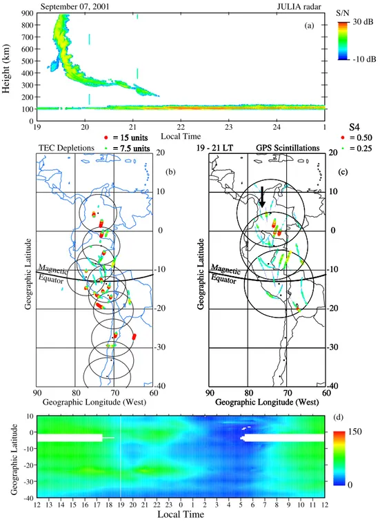
Fig. 4.The top panel shows range-time-intensity plot of a radar plume and a bottomside trace observed by the JULIA radar on 7 September
2001. The middle panels show maps of TEC depletions and GPS scintillations detected by the GPS receivers in South America. The lower panel displays absolute TEC latitudinal profiles measured between 12:00 LT on 7 September and 12:00 LT on 8 September 2001.
first in Ancon at 20:50 LT very close to the zenith direction. This depletion drifted through Pucallpa (21:20 LT), Bogota (21:38 LT), Iquitos (21:40 LT) and later Cuzco at 21:55 LT. The level of depletion in the northern crest (Bogota) was 60 TEC units. At Copiapo, near the southern crest of the anomaly the depletion was also 60 units, which indicates that the amount of depletion is approximately symmetric with re-spect to the magnetic equator. Nevertheless, as we will see in the following section, the TEC latitudinal profiles were
4 Case Studies
In Sect. 3 we presented TEC depletions observed near the anomaly crests that were as large as 60 TEC units in depth, but close to the magnetic equator the TEC depletions were only 20 TEC units or less. In this section, we introduce three case studies to confirm the inherent association between TEC depletions, GPS scintillations and radar plumes.
4.1 7 September 2001
Figure 4a shows the JULIA power map measured on 7 September 2001, in which we observed a single plume, ex-tending at least 900 km altitude at 19:30 LT. The correspon-dence of this radar plume and a TEC depletion containing low density plasma is demonstrated in Fig. 2c by the pres-ence of a 15-unit TEC depletion passing near Ancon, also at 19:30 UT. No additional plumes were seen at Jicamarca during the rest of the evening, although a bottomside trace was detected with JULIA lowering in altitude between 19:40 and 21:30 LT. In association with the bottomside trace, no TEC depletions were observed near the Jicamarca longitude. Nevertheless, other TEC depletions developed far to the east of the 76◦W meridian. Also significant was the absence of UHF scintillations (not shown here) after 20:00 LT at the An-con F7 sub-ionospheric intersection (see Fig. 1). This lack of UHF scintillations and the absence of TEC depletions larger than 2 TEC units, implied that the JULIA bottomside trace of 7 September 2001 was not associated with significantly large TEC depletions, and if 1-km irregularities existed, they were constrained to the bottomside F-region and probably generated a very low level of UHF scintillations below the detection threshold of the Ancon system.
Figure 4b displays the location and the magnitude of the TEC depletions that were identified in the TEC profiles for all stations and all satellites passes observed between 19:00 and 21:00 LT. This plot denotes three important features common to the three events presented in this section. First, the latitudi-nal extension of the TEC depletions is quite symmetric with respect to the magnetic equator. Secondly, the depth of the TEC depletion is less at the equator (<8 units) and larger at the crests (>30 units). Thirdly, the latitudinal extension of the depletions agrees quite well with the maximum latitude of scintillations.
Figure 4c shows the L1 GPS scintillations measured with the receivers deployed at Bogota, Iquitos and Cuzco between 19:00 and 21:00 LT. Scintillations from Pucallpa were not in-cluded due to the strong contamination of the S4 index pro-duced by signal multi-paths. The magnitude of the S4 index has been color coded according to the scale indicated in the upper right corner. The S4 scintillation index is equal to 0.4 at the location of the northern crest where the density is the largest, but decreases to 0.2 at the trough. The scintillations associated with the radar plume are seen to reach 16◦ mag-netic latitude (see arrow in Fig. 4c). A field line crossing the F-region at this latitude maps to an apex height of 1000 km. This maximum altitude inferred from the GPS scintillation
does not contradict the smaller apex altitude of the plume since the JULIA range-time plot was limited to 900 km.
Figure 4d shows a color-coded representation of the TEC values measured on 7 September 2001, plotted as a function of latitude and local time. At 19:00 LT, the TEC value near the magnetic equator (−12◦geographic latitude) diminished rapidly and the amplitude of the crests increased slightly, in-dicating a re-energization of the fountain effect and the de-velopment of a more pronounced anomaly. The anomaly re-mained visible until 02:00 LT, when the TEC latitudinal pro-files became more uniform and adopted a typical nighttime value of 15 units. On this day the anomaly was quite sym-metric, centered at the magnetic equator, and with both crests possessing nearly the same width.
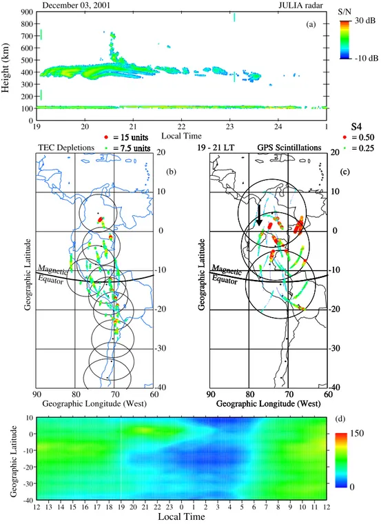
4.2 3 December 2001
Figure 5 shows the intensity of coherent echoes measured by JULIA on 3 December 2001, the locations of TEC deple-tions and GPS scintilladeple-tions superimposed on a geographic layout, and 24 h of TEC latitudinal profiles centered on lo-cal midnight. The JULIA map indicates the existence of a 100-km thick bottomside layer, which starts right after sun-set and lasts until 23;30 LT. A single radar plume appeared at 20:35 LT and extended up to 720 km altitude. GPS scin-tillations corresponding to this day (Fig. 5c) show that the latitudinal extension of scintillations has a strong variability as a function of longitude. It reaches 15◦magnetic latitude (MLAT) at 73◦W longitude, but only 13◦MLAT near the Ji-camarca longitude (see arrow). A plume rising to 720 km maps to 12.7◦MLAT, which is in very good agreement with
the maximum extension of GPS scintillations at the Jica-marca longitude. Figure 5b shows that on this day the TEC depletions have depths smaller than the depletions seen on 7 September 2001. The TEC depletions are 6 units near the equator and about 10 units at the anomaly, much smaller than 12 and>40 units that was seen at the equator and the crests on 7 September 2001. Notwithstanding, the GPS scintilla-tions of 3 December 2001 are more intense, containing S4 values near 0.6 at the northern crest and 0.4 near the trough. Another important difference is the low level of UHF scin-tillations that was detected on 7 September 2001 (S4=0.3) and the more intense (S4=0.7) and long lasting event of 3 December 2001. On the latter day, a decreasing level of scin-tillations was seen between 20:00 LT and the early morning hours (06:00 LT).
Figure 5.
19 20 21 22 23 24 1
0 100 200 300 400 500 600 700 800 900
30 dB S/N
-10 dB
Height (km)
December 03, 2001 JULIA radar
Local Time
(a)
90 80 70 60-40 -30 -20 -10 0 10 20
Geographic Longitude (West)
Geographic Latitude
(b)
Magnetic Equator TEC Depletions
= 15 units = 7.5 units = 15 units = 7.5 units = 15 units = 7.5 units = 15 units = 7.5 units = 15 units = 7.5 units = 15 units = 7.5 units = 15 units = 7.5 units = 15 units = 7.5 units = 15 units = 7.5 units = 15 units = 7.5 units
90 80 70 60-40 -30 -20 -10 0 10 20
Geographic Longitude (West)
Geographic Latitude
(c)
Magnetic Equator
GPS Scintillations 19 - 21 LT
S4 = 0.50 = 0.25
90 80 70 60-40 -30 -20 -10 0 10 20
Geographic Longitude (West)
Geographic Latitude
(c)
Magnetic Equator
GPS Scintillations 19 - 21 LT
S4 = 0.50 = 0.25
90 80 70 60-40 -30 -20 -10 0 10 20
Geographic Longitude (West)
Geographic Latitude
(c)
Magnetic Equator
GPS Scintillations 19 - 21 LT
S4 = 0.50 = 0.25
12 13 14 15 16 17 18 19 20 21 22 23 0 1 2 3 4 5 6 7 8 9 10 11 12 -40
-30 -20 -10 0 10
Local Time
Geographic Latitude
(d)
150
0
Fig. 5. Same as Fig. 4, but corresponding to 3 December 2001. The top panel shows a single radar plume developing at 20:40 LT, and
reaching 700 km. The TEC depletion and the GPS scintillations, at locations near Jicamarca, extend up to 13◦magnetic latitude. The TEC profiles seen near sunset are highly asymmetric. Nevertheless, strong scintillations were detected this day.
inhibit the growth of the equatorial plasma bubbles. How-ever, we did not observe an inhibition of the irregularities on 3 December 2001 and on many other nights, which are pre-sented below in Sect. 5. It has been recently suggested by Devasia et al. (2002) that the transequatorial wind may act as an instability suppressor but only when the F-region alti-tude is below a certain limit. This hypothesis could explain the maintenance of ESF during nights when the anomaly is
widely asymmetric. In Sect. 7, we put forth another hypothe-sis that might explain the variability of the TEC profiles that commonly exist during GPS scintillations events.
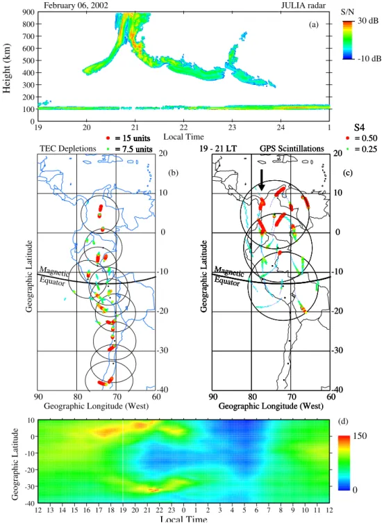
4.3 6 February 2002
19 20 21 22 23 24 1 0
100 200 300 400 500 600 700 800 900
30 dB S/N
-10 dB
Height (km)
February 06, 2002 JULIA radar
Local Time
(a)
90 80 70 60-40 -30 -20 -10 0 10 20
Geographic Longitude (West)
Geographic Latitude
(b)
Magnetic Equator TEC Depletions
= 15 units = 7.5 units = 15 units = 7.5 units = 15 units = 7.5 units = 15 units = 7.5 units = 15 units = 7.5 units = 15 units = 7.5 units = 15 units = 7.5 units = 15 units = 7.5 units = 15 units = 7.5 units = 15 units = 7.5 units
90 80 70 60-40 -30 -20 -10 0 10 20
Geographic Longitude (West)
Geographic Latitude
(c)
Magnetic Equator
GPS Scintillations 19 - 21 LT
S4 = 0.50 = 0.25
90 80 70 60-40 -30 -20 -10 0 10 20
Geographic Longitude (West)
Geographic Latitude
(c)
Magnetic Equator
GPS Scintillations 19 - 21 LT
S4 = 0.50 = 0.25
90 80 70 60-40 -30 -20 -10 0 10 20
Geographic Longitude (West)
Geographic Latitude
(c)
Magnetic Equator
GPS Scintillations 19 - 21 LT
S4 = 0.50 = 0.25
12 13 14 15 16 17 18 19 20 21 22 23 0 1 2 3 4 5 6 7 8 9 10 11 12 -40
-30 -20 -10 0 10
Local Time
Geographic Latitude
(d)
150
0
Fig. 6. Same as Fig. 4, but corresponding to 6 February 2002. The radar map shows two plumes. The first occurs between 20:40 and
21:10 LT and extends beyond 900 km. The TEC depletions and GPS scintillations detected at several sites extend up to 23 degrees magnetic latitude and indicate that the plasma bubbles extend up to 1400 km altitude.
extension of two radar plumes that developed from a bottom-side trace that was seen to continuously decrease in altitude. The first plume was seen at 21:00 LT, when the F-region bot-tomside had raised up to 600 km altitude. The strength of the echoes suggested that this plume extended well beyond the 900 km altitude limit of Fig. 6a. The second plume was detected at 23:00 LT and reached 700 km altitude. Figure 6b displays the geographic location of several TEC depletions measured by all ten GPS receivers. Similar to the other
two case-events, the magnitude of the depletions increased at latitudes further away from the equator, but in this event the depletions were seen up to 20◦N MLAT (8◦geographic lat) and 25◦S MLAT (38◦S geographic lat). The depletions
Figure 7.
TEC Units
150
0
6 5 4 3 2 1 0
10 0 -10 -20 -30 -40
September 08, 2001
Universal Time
Geographic Latitude
6 5 4 3 2 1 0
10 0 -10 -20 -30 -40
September 25, 2001
Universal Time
Geographic Latitude
6 5 4 3 2 1 0
10 0 -10 -20 -30 -40
October 22, 2001
Universal Time
Geographic Latitude
6 5 4 3 2 1 0
10 0 -10 -20 -30 -40
October 25, 2001
Universal Time
Geographic Latitude
6 5 4 3 2 1 0
10 0 -10 -20 -30 -40
December 05, 2001
Universal Time
Geographic Latitude
6 5 4 3 2 1 0
10 0 -10 -20 -30 -40
December 18, 2001
Universal Time
Geographic Latitude
6 5 4 3 2 1 0
10 0 -10 -20 -30 -40
December 19, 2001
Universal Time
Geographic Latitude
6 5 4 3 2 1 0
10 0 -10 -20 -30 -40
January 15, 2002
Universal Time
Geographic Latitude
6 5 4 3 2 1 0
10 0 -10 -20 -30 -40
January 18, 2002
Universal Time
Geographic Latitude
6 5 4 3 2 1 0
10 0 -10 -20 -30 -40
January 22, 2002
Universal Time
Geographic Latitude
6 5 4 3 2 1 0
10 0 -10 -20 -30 -40
February 02, 2002
Universal Time
Geographic Latitude
6 5 4 3 2 1 0
10 0 -10 -20 -30 -40
February 10, 2002
Universal Time
Geographic Latitude
6 5 4 3 2 1 0
10 0 -10 -20 -30 -40
October 12, 2001
Universal Time
Geographic Latitude
6 5 4 3 2 1 0
10 0 -10 -20 -30 -40
November 07, 2001
Universal Time
Geographic Latitude
6 5 4 3 2 1 0
10 0 -10 -20 -30 -40
February 19, 2002
Universal Time
Geographic Latitude
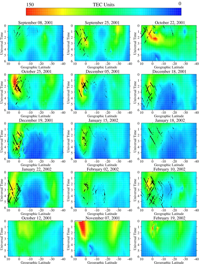
Fig. 7.Absolute TEC distributions for 15 case study events observed during the equinox and December solstice seasons. The first 12 cases
equator. UHF scintillations, measured at Ancon with the 250 MHz system, were also much stronger than the previous two cases. The UHF scintillations detected at both F7 and F8 sub-ionospheric penetration points contained several bursts of saturated values. The TEC profiles of Fig. 6d indicates that the TEC anomaly becomes more pronounced and separated from the magnetic equator at 17:00 LT. Both crests are dis-placed at least 19◦MLAT away from the magnetic equator at 22:00 LT. This event displays one of the largest anomaly dis-placements that we have seen. The location of the crests 19◦ away from the magnetic equator correlates quite well with the largest latitudinal extensions of scintillations. Right after 22:00 LT, both crests retracted and moved closer to the mag-netic equator until 01:00 LT when they faded. We interpret that this separation of the crests of the anomaly is the result of a strong fountain effect, driven by a large vertical drift that was most likely directed upwards until 22:00 LT when it reversed to a downward direction.
5 Simultaneous observations of TEC and GPS scintilla-tions
Figure 7 shows the temporal evolution of the TEC profiles for 15 days selected between the months of September 2001 and February 2002. The TEC values presented in this fig-ure correspond to the first 6 h of the evening, starting after local sunset (00:00 UT). The dark traces superimposed on the color-coded TEC data illustrate the scintillation S4 index measured at Bogota, Iquitos and Cuzco. They are placed at the latitude of the sub-ionospheric penetration point and at the times when the S4 index exceeded the noise level (0.20). The purpose of this figure is: 1) to demonstrate the close rela-tionship between the location of scintillations and the latitu-dinal extension of the equatorial anomaly, and 2) to indicate the rapid response of GPS scintillations to the evolution of the TEC profiles. The 12 frames in the four upper rows show data for days with scintillation activity. The three frames in the bottom row are for nights with no scintillation activity. It is worthwhile to note that between 00:00 and 06:00 UT the nighttime F-region normally decays in a slow manner. In ad-dition, during the early evening hours there commonly exists a rapid plasma re-distribution along the field lines: the foun-tain effect. An upward drift near the equator drives the direct fountain effect (Hanson and Moffett, 1966) by moving the plasma poleward, reinforces the amplitude of the crests, and reduces the density at the trough. A downward vertical ve-locity creates a reverse fountain effect (Sridharan et al., 1993; Balan and Bailey, 1995), moves both crests equatorward, di-minishes the size of the crests, and increases the TEC value at the trough.
The frame labeled 8 September 2001 (7 Sept 2001 in local time), placed in the upper left corner, reproduces the TEC lat-itudinal profiles of Fig. 4d, but here we introduce the scintil-lation information within the context of the TEC variability. GPS scintillations appeared at 00:00 UT, when the TEC crest was fairly constant; the trough TEC value was small and the
September 2001
01 02 03 04 05 06 07 0809 10 11 12 13 14 15 16 17 18 19 20 21 2223 24 25 26 27 28 29 30
25 20 15 10 5 0 -5 -10 -15 -20
MLAT
September 2001
01 02 03 04 05 06 07 0809 10 11 12 13 14 15 16 17 18 19 20 21 2223 24 25 26 27 28 29 30
25 20 15 10 5 0 -5 -10 -15 -20
MLAT
December 2001
01 0203 0405 0607 08 0910 1112 1314 15 1617 1819 2021 22 2324 2526 27 2829 3031
25 20 15 10 5 0 -5 -10 -15 -20
MLAT
December 2001
01 0203 0405 0607 08 0910 1112 1314 15 1617 1819 2021 22 2324 2526 27 2829 3031
25 20 15 10 5 0 -5 -10 -15 -20
MLAT
January 2002
01 0203 0405 0607 08 0910 1112 1314 15 1617 1819 2021 22 2324 2526 27 2829 3031
25 20 15 10 5 0 -5 -10 -15 -20
MLAT
January 2002
01 0203 0405 0607 08 0910 1112 1314 15 1617 1819 2021 22 2324 2526 27 2829 3031
25 20 15 10 5 0 -5 -10 -15 -20
MLAT
February 2002
01 02 03 04 05 06 07 08 09 10 11 12 13 14 15 16 17 18 19 20 21 22 23 24 25 26 27 28
25 20 15 10 5 0 -5 -10 -15 -20
MLAT
February 2002
01 02 03 04 05 06 07 08 09 10 11 12 13 14 15 16 17 18 19 20 21 22 23 24 25 26 27 28
25 20 15 10 5 0 -5 -10 -15 -20
MLAT
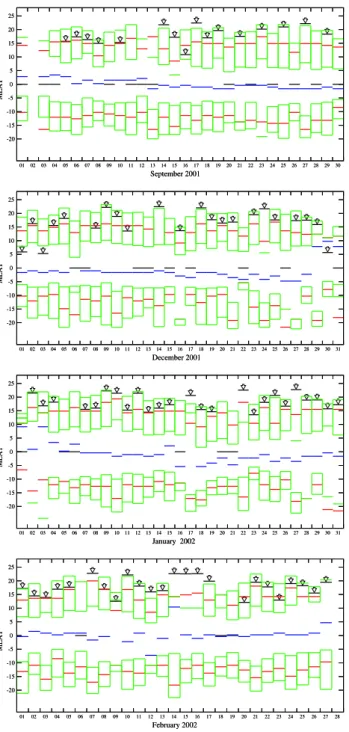
Fig. 8.Latitudinal distribution of the location of the anomaly for the
months of September, December, January and February. The blue trace near 0◦magnetic latitude indicates the location of the trough. The red lines are used to point out the locations of the anomaly crests. The green lines indicate the extension where the crests di-minish 50%. The short black lines and the arrows seen near the northern boundary of the northern crest indicate the maximum lat-itude of GPS scintillations. Note that only in a few cases does the maximum latitude of scintillations extend beyond the limits of the anomaly.
the anomaly peak and weak scintillations within the trough region. The frame for 22 January 2002 shows the northern crest of the anomaly displaced up to 19◦magnetic latitude and GPS scintillations extending beyond our latitudinal
cov-erage. The frame for 2 February 2002 shows the crests of the anomaly placed near 13◦magnetic latitude and the GPS
scintillations confined to a maximum latitudinal extension of 14◦ magnetic latitude. On this day scintillations ceased at
05:30 UT during a period when the reverse fountain was in effect. The frame corresponding to 10 February 2002 shows a pattern of strong scintillations that initiated at 01:00 UT. At this time, there is a re-initiation of the fountain effect, shown as a decrease of the TEC trough and an increase of the northern crest. Nevertheless, GPS scintillations persisted for several hours after the anomaly had started retracting equa-torward. On this day, GPS scintillations were observed to extend beyond the limit of northern boundary of the north-ern crest (22◦MLAT). However, the southern crest reached a larger magnetic latitude equal to 27◦.
All three cases displayed in the bottom row were not as-sociated with GPS and UHF scintillations at all the stations. The salient feature seen in all three panels is the relatively high level of TEC values at the magnetic equator (∼12◦S).
The plot for 12 October 2001 shows a fairly uniform TEC latitudinal distribution. In this plot a modest TEC increase occurs between 0◦ and 6◦S at 01:00 UT. The profiles for 7 November 2001 show two well-defined crests and a promi-nent northern peak, but the trough is quite broad with a TEC value above 70 TEC units. The event of 19 February 2002 shows a quasi-uniform TEC distribution with a narrow and short-lived crest. The cases presented in Fig. 7 summarize the great variability of the TEC profiles during 15 nights when all 10 GPS receivers were operating concurrently.
6 Statistics
Figure 8 presents the day-to-day variability of the extension of the equatorial anomaly measured at 20:00 LT. This time commonly corresponds to the initiation of ESF/scintillations. Figure 8 displays the magnetic latitude of the location of both crests of the anomaly (red traces), the trough (blue trace), and the 50% amplitude decay of the crests (green boxes). We also indicate the northern edge of the region subject to GPS scin-tillations using a bold line and an arrow. The scintillation information originates from real-time calculations of the S4 index based on the 10-Hz amplitude of the L1 GPS signal recorded at three of the stations (Bogota, Iquitos and Cuzco). Their combined scintillation-observing range stretches be-tween 21◦S and 12◦N geographic latitude. Days without
0 5 10 15 20 25 5
10 15 20 25
MLAT
# of events
Scintillation Max Lat
0 5 10 15 20 25 8
16 24 32 40
MLAT
Anomaly Northern Boundary
-10 -5 0 5 10 15 5
10 15 20 25
MLAT Difference (Crest-Scin)
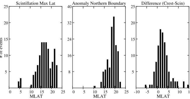
Fig. 9.The left histogram shows the maximum latitude of scintillations. The center panel displays the location of the northern boundary of
the anomaly, defined as the poleward edge where the northern crest decreases 50% of its peak value. The right panel exhibits the distribution of the difference between poleward boundary of the anomaly and the maximum latitude of scintillations. Only in 9 cases out of 100 were GPS scintillations (and TEC depletions) seen poleward of the northern boundary of the anomaly.
was observed, most of the days, close to the magnetic equa-tor. Exceptions are seen in early September, late December, 16–20 January and 12 and 27 February when the trough was displaced up to 7◦from the magnetic equator. The location and width of the crests also show a large degree of variabil-ity. In some cases, both crests of the anomaly are close to 10◦ magnetic latitude, as seen on 8 and 26 September, 17 December, 23 January, and 12 February. But, on other occa-sions, they are nearly at 20◦, as seen on 10 and 22 January and 7 February. The width of the crests were calculated by taking the difference between the crest and the trough TEC values, and recording the latitude where this difference falls off by 50%. It is evident that for most of the days the northern and southern crests are not placed symmetrically with respect to the magnetic equator and do not have the same latitudinal span. The maximum latitude of scintillations also shows a great variability; sometimes it is only 5◦from the magnetic equator. But in other cases scintillations reach 23◦magnetic latitude; this latitude corresponds to the poleward limit of the combined field-of-view of the GPS network. There is no doubt that, for some of these events, scintillations and the anomaly continue extending further poleward, but these regions were beyond the observing boundaries of the exist-ing chain of GPS receivers. Durexist-ing the 6-month period pre-sented in this paper, we found that on 40 nights (22% of all days) scintillations extended up to a latitude equal or greater than 20◦away from the magnetic equator. We also observed
that while the amplitude of the crests show a prominent sea-sonal variability, the latitudinal location and extension of the anomaly display no significant seasonal dependence. We have also detected that for all months involved in this study,
the northern crest was displaced toward more poleward lati-tudes than the southern peak of the anomaly.
Figure 9 illustrates the statistical distribution of the latitu-dinal extension of scintillations, the latitude of the anomaly northern boundary and a cross-comparison between them. The histogram on the left side reveals that for the majority of days, scintillations are confined to a magnetic latitude range that varies between 10◦and 23◦. Nevertheless, there
19 20 21 22 23 0 1 2 3 200
300 400 500 600 700
Local Time
Bogota
Altitude (km)
GPS Scintillation
19 20 21 22 23 0 1 2 3
200 300 400 500 600 700
Local Time
Iquitos
Altitude (km)
GPS Scintillation
19 20 21 22 23 0 1 2 3
200 300 400 500 600 700
Local Time
Cuzco
Altitude (km)
GPS Scintillation
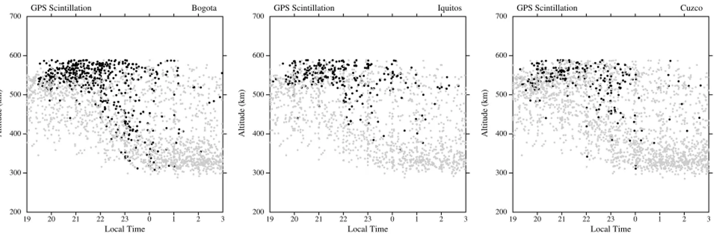
Fig. 10.hmF2 value of the equatorial ionosphere during the ten-month observational period presented in this study. The gray dots correspond
to events when the GPS scintillation index was below 0.20. The black dots are for S4 levels above 0.20.
Figure 10 displays a mass plot of the altitude of the F-region peak measured by the Jicamarca digisonde between the months of September 2001 and June 2002. The peak altitude (hmF2) is plotted as a function of local time start-ing near local sunset. ThehmF2 values are calculated with the Artist software that runs simultaneously with the data ac-quisition process. Different gray shading is used to distin-guish between the absence (light gray) and presence (black) of GPS scintillation. Each panel of Fig. 10 shows thehmF2 values binned as a function of the scintillation activity mea-sured by the receivers placed at Bogota, Iquitos and Cuzco. Similar to results published by other researchers, we found a well-defined dependence of the appearance of GPS scintil-lations and the altitude of the F-layer. Between 19:00 and 21:30 LT, scintillations mostly appear when the layer is lo-cated above 500 km altitude. Nevertheless, a small number of events occur whenhmF2 is less than 500 km altitude. At local times later than 21:30 LT, the relative number of scintil-lation events withhmF2 below 500 km drastically increases, as it is common to observe scintillations at altitudes varying between 300 and 500 km. These events probably correspond to cases that outlived the descent of the F-region, and scintil-lations persisted during the nighttime decay. This feature is common to all three stations and usually starts near 21:30 LT. During the descent of the F-region, we found that the number of scintillation events detected at Cuzco, near the magnetic equator, was smaller than the number of events at other sta-tions. This result is probably due to the much smaller density at the trough that makes the S4 level significantly close to the noise level. Figure 11 displays the altitude of the F-layer for all instances when TEC depletions were detected at the Bo-gota, Iquitos, Pucallpa, and Iquique stations. The red dots indicate cases when the depth of the depletions were larger than 30 TEC units. The blue dots are for depletions less than 30 units. The distribution ofhmF2 is quite similar to the dis-tributions of Fig. 10 for GPS scintillations. Figures 10 and 11 demonstrate that equatorial plasma bubbles can survive up to 2 hours after the nighttime F-layer starts descending. We also indicate that plasma bubbles and GPS scintillations rapidly
decay when the equatorial F-layer reaches 300 km altitude. For days when thehmF2 remains at altitudes above 500 km, scintillations and TEC depletions seem to last for longer pe-riods and can be seen as late as 03:00 LT. The occurrence of GPS scintillations and TEC depletions when the F-region peak was below 500 km altitude warrants further study of the background conditions of the ionosphere during these cases. A very informative statistics of the preferred ionospheric conditions that prevailed during the occurrence of scintilla-tion/depletion events is presented in Fig. 12. This figure shows the hmF2 measured at Jicamarca as a function of two key representative parameters of the TEC profiles: the crest-to-trough TEC ratio and the latitudinal separation of the northern crest. The left panel shows thehmF2 versus the crest-to-trough ratio binned according to the presence (red and blue dots) and absence of scintillation (gray dots). The right panel displays the peak altitude as a function of the crest separation in degrees. Figures 12a and 12b were constructed by estimating the maximum level of scintillations every hour the Bogota and Iquitos GPS receivers operated between sun-set (∼19:00 LT) and 23:00 LT. Each scintillation value was paired with the corresponding F-region peak altitude mea-sured at Jicamarca and the TEC latitudinal profile recorded with the GPS network. The red dots illustrate scintillation events observed before 22:00 LT, and the blue dots represent scintillation cases occurring before 23:00 LT. Figure 12 re-veals that when the equatorial F-region peak is above 500 km, GPS scintillations are able to develop for TEC ratios as small as 1.25 or as large as 6.0, and crest separations between 6◦
and more than 20◦. But as the peak altitude becomes less
19 20 21 22 23 0 1 2 3 200
300 400 500 600 700
Local Time
Bogota
Altitude (km)
TEC Depletion
19 20 21 22 23 0 1 2 3
200 300 400 500 600 700
Local Time
Iquitos
Altitude (km)
TEC Depletion
19 20 21 22 23 0 1 2 3
200 300 400 500 600 700
Local Time
Pucallpa
Altitude (km)
TEC Depletion
19 20 21 22 23 0 1 2 3
200 300 400 500 600 700
Local Time
Iquique
Altitude (km)
TEC Depletion
Fig. 11. hmF2 values measured during the occurrence of TEC depletions measured with the network of GPS receivers. TEC depletions
larger than 30 TEC units are depicted as red dots; values smaller than 30 units are indicated by blue dots. Mass plots for only 4 stations are presented here.
The inclined line in each panel depicts the best fit to these minimum points. These traces also indicate the almost lin-ear relationship between the minimum crest separation (and crest/trough ratio) and the altitude of the F-region for all the scintillations events that were observed at Bogota and Iqui-tos. It is important to mention that most of the gray dots (times of no scintillations) are observed bunched at TEC ra-tios less than 2.2. Based on this data, it is possible to con-clude that an equatorial F-region peak below 500 km does not necessarily imply an inhibition of the onset or persistence of GPS scintillation, but it does require the crest/trough TEC ratio to be 2 or higher and the crest separation to exceed 8◦. The lower the F-region peak, the higher that the TEC ratio
and the crest separation have to be for the flux tube to remain unstable to the initiation or persistence of GPS scintillations.
7 Discussion
300 400 500 600
1.0 1.5 2.0 2.5 3.0 3.5 4.0 4.5 5.0 5.5 6.0 TEC/TEC(eq)
Bogota - Iquitos
Altitude (km)
GPS Scintillation (a)
300 400 500 600
1.0 1.5 2.0 2.5 3.0 3.5 4.0 4.5 5.0 5.5 6.0 3006 8 10 12 14 16 18 20 22 24 26
400 500 600
Lat(N. Crest) - Lat(Eq)
Bogota - Iquitos
Altitude (km)
GPS Scintillation (b)
6 8 10 12 14 16 18 20 22 24 26
300 400 500 600
Fig. 12.Distribution of thehmF2 values as a function of the crest-to-trough ratio (panel(a)and vs. the crest separation (panel(b)), binned
according to the presence (colored dots) and absence of GPS scintillations (gray dots). The inclined lines in the left part of each frame have been fitted to the minimum values of the crest/trough ratio (or crest separations) for different altitude sectors.
signal from the same GPS satellite is recorded at different stations. One of the physical properties inferred from the TEC data is the determination of the location where a bub-ble is triggered. Figures 3a, 3b and 3e (corresponding to Bo-gota, Iquitos and Cuzco) observed 2 TEC depletions between 19:00 and 22:00 LT; contrary to this, Figs. 3c and 3d (Pu-callpa and Ancon) showed only one depletion. This fact in-dicated that the TEC depletion seen at Iquitos between 20:20 and 20:42 LT, which was also observed in Bogota between 20:30 and 20:53 LT, most likely originated in a location be-tween Pucallpa and Iquitos. The depletion seen at Pucallpa between 21:08 and 21:47 LT could not be associated with the plasma bubble recorded much earlier at Iquitos and Bo-gota since the plasma depletions were drifting eastward. The average drift of the background plasma is another physical parameter that can be calculated using the arrival time of the TEC depletion as it moves from one station to another lo-cated further east. TEC observations from 2 stations lolo-cated near the magnetic equator such as Ancon and Cuzco (Figs. 2c and 2d) show the passage of a TEC depletion crossing their ionospheric intersections with relatively small changes in the shape of the depletion. We determined a velocity equal to 140 m/s using the time elapsed between the TEC minima at Ancon and Cuzco and the east-west distance between the sta-tions. In agreement with this value, the UHF spaced-receiver scintillation system that operates at Ancon (Valladares et al., 1996) measured a zonal drift equal to 160 m/s at 22:10 LT. The third geophysical parameter that we calculated was the westward tilt of the plasma bubbles. Comparison of the TEC curves measured at Cuzco, Iquitos and Bogota indicated the passage of a TEC depletion at times that were consistent with
to generate irregularities on the west wall of a plasma bub-ble. A zonal neutral windUis also able to produce struc-tures under the conditionU·∇n<0 , which for an eastward wind corresponds again to the westward wall. Based on their computer calculations Zalesak et al. (1982) indicated that the westward as well as the eastward wall could be subject to secondary instabilities. These authors included the tilt of the plumes and suggested that at high altitudes the normally sta-ble east wall orients out of the purely vertical direction and becomes unstable to the gravitational and gradient-drift in-stabilities. More refined statistical analysis of these geophys-ical parameters will be exploited in the future to investigate the evolution and lifetime of the plasma bubbles and their associated scintillations.
By using data collected by the JULIA radar, along with TEC and GPS scintillations, we have constructed a very com-plete diagnostic of the background and the turbulent state of the nighttime low-latitude ionosphere for three different days. The radar coherent echoes, TEC depletions, GPS scin-tillations, and the TEC latitudinal profiles of Figs. 4, 5, and 6 portray the seasonal and day-to-day variability of the equato-rial irregularities at different scale sizes. The following fea-tures were consistently observed in all three figures: 1) The location and the depth of the TEC depletions were approximately symmetric with respect to the magnetic equa-tor, even when the background TEC was not symmetric. The absence of GPS scintillation measurements south the mag-netic equator prevented us from investigating the symmetry of this parameter. 2) The depth of the TEC depletions and the intensity of GPS scintillations were larger at the crests of the anomaly than at the trough. 3) The latitudinal extension of the locations of the TEC depletions was equal to the ex-tension of GPS scintillations. 4) Radar plumes were always collocated with TEC depletions and GPS scintillations. In addition, when the JULIA radar observed bottomside traces, these were not observed to be associated with GPS scintil-lations. The latter two experimental facts reaffirm the theo-retical predictions of Costa and Kelley (1976) and previous observations conducted by Basu et al. (1986). The presence of the largest depletion depths at the crests of the anomaly is probably a consequence of the density along the depleted flux tubes being almost constant (Hanson and Bamgboye, 1984). Because the background undisturbed density is the largest at the crests, then a more dense region will be evacu-ated by the instability process, resulting in a much deeper depletion. Recently, Keskinen et al. (2003) have studied the three-dimensional nonlinear evolution of plasma bubbles and demonstrated that the sharpest density gradients exist at equatorial anomaly latitudes. We found that indeed GPS scintillations were more prominent near the crest, but when a single station was considered, we found no firm assurance that deeper TEC depletions correlate with more intense GPS scintillations. In fact, by comparing Figs. 4 and 5 the op-posite correspondence seems to be valid. Figure 2 shows a 20-unit depletion that was observed at Cuzco on 7 Septem-ber 2001. This depletion was accompanied with a S4 index near the noise level (0.20). In comparison, a smaller 12-unit
noticed that on these two days, the southern crest reached more poleward latitudes than the northern peak. This again reinforces the need to conduct the field line integration from end-to-end of the flux tube. We suggest that this relation-ship between the latitudinal width of the anomaly and the extension of GPS scintillations seems to be necessary condi-tions for all local times, all magnetic condicondi-tions, and proba-bly all solar activity epochs. The bottom row of Fig. 7 has shown the TEC distributions for 3 days when no GPS scin-tillations were detected. The common feature on all 3 days was the large TEC value (>75 units) at the trough and the crest/trough ratio less than 2. This behavior of a stable equa-torial ionosphere is in agreement with the conditions of the TEC profiles put forth by Valladares et al. (2001). Figure 7 also introduced the role of the reverse fountain effect, act-ing as a suppressor of plasma bubbles and GPS scintillations. The initiation of the reverse fountain was illustrated in Fig-ure 4a in which a bottomside trace was observed to be mov-ing rapidly downward after 19:30 UT. Simultaneously, the TEC latitudinal profiles indicated an increase in the TEC val-ues near the magnetic equator. We have observed that GPS scintillations can be inhibited right after the start of the re-verse fountain effect; but can also decay 1–2 h afterwards. Below we explain how the re-distribution of plasma along the field lines can make the equatorial ionosphere become stable to the RTI and are able to suppress or extinguish ESF irregularities. We did not expect to find the strong asymme-try of the TEC profiles that prevailed during the December solstice, even during days when the latitudinal distribution of the TEC depletions was symmetric with respect to the magnetic equator. On many days, GPS scintillations, TEC depletions, and radar plumes were detected even when the southern crest was absent. The main contributor to the asym-metry of the anomaly is the meridional wind that during the December solstice blows from south to north (Walker et al., 1994). Other factors may be an asymmetrical distribution of the O/N2 ratio or latitudinal gradients of the zonal or vertical neutral wind.
Figures 8 and 9 indicated that sometimes GPS scintilla-tions could be detected poleward of the 50% decay of the northern crest. In fact, a total of 9 cases were found during the analysis of this limited data set. We noticed that dur-ing these nine days the poleward boundary of the southern crest was displaced to even higher magnetic latitudes than the poleward boundary of the northern crest. This will def-initely augment the flux-tube integrated conductivity of the field line that intersects the poleward boundary of the GPS scintillations. In summary, Figs. 7, 8 and 9 reaffirm that the stability of the flux tube is a non-local phenomenon that de-pends on the density along the whole flux tube.
Figure 12 indicated that when the equatorial F-region peak is above 500 km, the low-latitude ionosphere is inherently unstable to the onset of the RTI. Then, if gravity waves (Kelley et al., 1981; Hysell et al., 1990) are present, GPS scintillations and plasma bubbles will develop. But as the F-region descends toward lower apex altitudes, the require-ment for ESF turbulence becomes more stringent, and larger
crest/trough TEC ratios and more widely separated crests are needed for the ionosphere to remain unstable. Figure 13 presents the schematic representations of the ionospheric densities for two different scenarios in which the nighttime F-region can be considered disturbed. These plots display a north-south 36◦-segment of the equatorial ionosphere cen-tered at the magnetic equator. Four field lines with apex alti-tudes varying from 500 km to 2000 km are indicated in each of the two frames. Both plots have been properly scaled to depict horizontal and vertical distances proportionally. The circular segment near the lower boundary represents the sur-face of the Earth. The numbers under this curve show the geographic latitude at the 76◦W meridian. The main dif-ferences between these two frames are the altitude of the F-region at the magnetic equator and the poleward extension of the anomaly. The left frame shows a density distribution that contains an equatorial F-region peaking at 750 km alti-tude and the crests separated by 8◦from the magnetic
equa-tor. The right frame displays the F-regionhmF2 at 400 km altitude, and the anomaly extending up to 15◦. Although the
0 0
500 500
1000 1000
1500 1500
2000 2000
Height (km)
2000 1000 0 -1000 -2000
0
-10
-20
0 0
500 500
1000 1000
1500 1500
2000 2000
Height (km)
2000 1000 0 -1000 -2000
0
-10
-20
0 0
500 500
1000 1000
1500 1500
2000 2000
Height (km)
2000 1000 0 -1000 -2000
0
-10
-20
0 0
500 500
1000 1000
1500 1500
2000 2000
Height (km)
2000 1000 0 -1000 -2000
0
-10
-20
Fig. 13.Schematic representation showing two possible scenarios of the latitudinal distribution of the F-region densities during events that
support the initiation and the development of plasma depletions. Note the difference in the altitude of the F-region near the magnetic equator and the locations of the Anomaly crests.
Nevertheless, after sunset the F-layer is reduced in depth and the TEC becomes a good representation of the density. We emphasize that the three parameters mentioned above can be used as a proxy for the initiation and persistence of equatorial plasma bubbles.
8 Conclusions
The investigation has led to the following:
1. We have shown that independent measurements of the same TEC depletion by two GPS receivers displaced in longitude can be employed to estimate the eastward mo-tion of the background ionosphere. GPS receivers dis-placed in latitude can also provide the tilt of the plasma plumes. We demonstrated that in some instances GPS receivers indicate the place and time of bubble initia-tion.
2. The three case-study events presented here have demon-strated the temporal and spatial correspondence be-tween radar plumes, GPS scintillations and TEC deple-tions. This fact supports the use of several GPS receiver sites to monitor the maximum altitude of the plasma bubbles.
3. We did not find a direct relationship between the depth of the TEC depletion and the intensity of GPS scintilla-tions. Nevertheless, more intense coherent echoes were observed when deeper TEC depletions transited above the JULIA radar.
4. At Bogota, GPS scintillations were seen on both walls of the TEC depletions. At Iquitos and Cuzco scin-tillations mainly occurred in the west side of the de-pletions. This latitudinal distribution of scintillations is in accord with predictions presented by Zalesak et al. (1982) based on numerical simulations of the evolu-tion of plasma bubbles.
5. We detected strong levels of GPS scintillation and deep TEC depletions when the TEC latitudinal profiles were symmetric, asymmetric, or even when one of the crests was absent. This fact indicates the importance of flux-tube integrated quantities to assess the stability of the equatorial F-region (Sultan, 1996).
6. There exists a prominent day-to-day variability in the location and width of the crest. The trough is princi-pally located near the magnetic equator, but it contains a 2◦dispersion with respect to the equator. The crests lo-cations typically vary between 10◦and 18◦of magnetic latitude, but could be as small as 5◦from the magnetic equator.
7. The poleward boundary of GPS scintillations and TEC depletions were bounded 90% of the days to the re-gions where the equatorial anomaly decreased 50% of the peak value. Weak level of scintillations were seen near the trough, but much higher values (>0.8) were ob-served at the crests during this period of solar maximum conditions.