www.geosci-model-dev.net/9/1143/2016/ doi:10.5194/gmd-9-1143-2016
© Author(s) 2016. CC Attribution 3.0 License.
Validation of the ALARO-0 model within the EURO-CORDEX
framework
Olivier Giot1,2, Piet Termonia1,3, Daan Degrauwe1, Rozemien De Troch1,3, Steven Caluwaerts3, Geert Smet1, Julie Berckmans1,2, Alex Deckmyn1, Lesley De Cruz1, Pieter De Meutter1,3, Annelies Duerinckx1,3, Luc Gerard1,
Rafiq Hamdi1, Joris Van den Bergh1, Michiel Van Ginderachter1,3, and Bert Van Schaeybroeck1
1Royal Meteorological Institute, Brussels, Belgium
2Centre of Excellence PLECO (Plant and Vegetation Ecology), Department of Biology, University of Antwerp, Wilrijk, Belgium
3Department of Physics and Astronomy, Ghent University, Ghent, Belgium
Correspondence to:Olivier Giot ([email protected])
Received: 29 July 2015 – Published in Geosci. Model Dev. Discuss.: 1 October 2015 Revised: 3 March 2016 – Accepted: 4 March 2016 – Published: 30 March 2016
Abstract. Using the regional climate model ALARO-0, the
Royal Meteorological Institute of Belgium and Ghent Uni-versity have performed two simulations of the past observed climate within the framework of the Coordinated Regional Climate Downscaling Experiment (CORDEX). The ERA-Interim reanalysis was used to drive the model for the pe-riod 1979–2010 on the EURO-CORDEX domain with two horizontal resolutions, 0.11 and 0.44◦. ALARO-0 is
char-acterised by the new microphysics scheme 3MT, which al-lows for a better representation of convective precipitation. In Kotlarski et al. (2014) several metrics assessing the per-formance in representing seasonal mean near-surface air tem-perature and precipitation are defined and the corresponding scores are calculated for an ensemble of models for differ-ent regions and seasons for the period 1989–2008. Of special interest within this ensemble is the ARPEGE model by the Centre National de Recherches Météorologiques (CNRM), which shares a large amount of core code with ALARO-0.
Results show that ALARO-0 is capable of representing the European climate in an acceptable way as most of the ALARO-0 scores lie within the existing ensemble. However, for near-surface air temperature, some large biases, which are often also found in the ARPEGE results, persist. For pre-cipitation, on the other hand, the ALARO-0 model produces some of the best scores within the ensemble and no clear re-semblance to ARPEGE is found, which is attributed to the inclusion of 3MT.
Additionally, a jackknife procedure is applied to the ALARO-0 results in order to test whether the scores are ro-bust, meaning independent of the period used to calculate them. Periods of 20 years are sampled from the 32-year sim-ulation and used to construct the 95 % confidence interval for each score. For most scores, these intervals are very small compared to the total ensemble spread, implying that model differences in the scores are significant.
1 Introduction
The climate projections used in the Fifth Assessment Re-port (AR5) of the Intergovernmental Panel on Climate Change (IPCC, 2013) are based on the set of global climate model (GCM) simulations performed within the fifth Cou-pled Model Intercomparison Project (CMIP5; Taylor et al., 2011). The horizontal resolution of the contributing GCMs is limited to typically 1–2◦by computational constraints. For
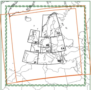
The Coordinated Regional Climate Downscaling Experi-ment (CORDEX; Giorgi et al., 2009) aims to perform both empirical–statistical downscaling and regional climate sim-ulations on different areas across the globe using an ensem-ble of RCMs. By prescribing several integration domains and resolutions, a direct quantitative comparison between the par-ticipating models’ performances and projections is feasible. The domain of interest in this study, is the EURO-CORDEX domain shown in Fig. 1 (inner orange box). Several RCM groups have performed simulations on this domain with hor-izontal resolutions of both 0.11 and 0.44◦.
All RCMs have a history in Numerical Weather Predic-tion (NWP) and often consist of a modified NWP code which is further developed separately from or parallel to the NWP code, borrowing for example its dynamical core but using different physics parameterisations or surface schemes (Dud-hia, 2014). In the present day, NWP limited area models (LAMs) are designed for resolutions down to a few kilo-metres, with adapted physics parameterisation schemes. At even higher resolutions, these models can (partly) resolve clouds and convective systems. Since a correct treatment of the cloud feedback is of critical importance for climate modelling (e.g. Sun et al., 2009; Lin et al., 2014), some of these NWP models have been used in climate mode: stud-ies by De Meutter et al. (2015), Hohenegger et al. (2008), Kendon et al. (2012) and Chan et al. (2014), where mod-els with resolution at the kilometre scale are used with-out convection parameterisation, show a better representa-tion of the intensity of extreme precipitarepresenta-tion, the diurnal cy-cle, afternoon convection onset and less drizzle. For instance, ALADIN-CLIMATE of the Centre National de Recherches Météorologiques (CNRM; Spiridonov et al., 2005) is a cli-mate version of the ALADIN limited area model that has been developed in the context of the international ALADIN consortium (ALADIN international team, 1997).
Over the past decade, within the context of the ALADIN consortium, a physics parameterisation scheme called 3MT (Modular Multiscale Microphysics and Transport) has been developed and used as the central feature of a new NWP model, ALARO-0 (Gerard and Geleyn, 2005; Gerard, 2007; Gerard et al., 2009). It is based on a parameterisation of deep convection and optimally adapted to be used at res-olutions in the so-called grey zone. Several countries have used and tested the model for operational weather forecast-ing and regional climate studies. The main feature of 3MT is scale awareness, i.e. the parameterisation itself works out which processes are unresolved at the current resolution, in contrast to traditional parameterisations which are switched on or off or have different tuned parameter values at differ-ent resolutions. This allows 3MT to generate consistdiffer-ent re-sults across scales, as shown by De Troch et al. (2013) in an extended downscaling experiment covering the period from 1961 to 1990. In their study, for every day, short-term sim-ulations were performed at different horizontal resolutions between 40 and 4 km. Both the initial and lateral boundary
BI
IP FR
ME SC
AL
MD EA
Figure 1. Domain boundaries of the used integration grids. The CORDEX community prescribes the rotated lat–long EURO-CORDEX domain (inner orange box) which is completely encom-passed by the E-OBS domain (outer orange box). The outer green boxes show the 11 (dashed lines) and RMIB-UGent-44 (full lines) conformal Lambert domain boundaries. The inner green boxes exclude the eight grid point Davies coupling zone. In black the different European climatic regions as defined in Chris-tensen and ChrisChris-tensen (2007) are shown (BI: the British Isles, IP: the Iberian Peninsula, FR: France, SC: Scandinavia, ME: mid-Europe, AL: the Alps, MD: the Mediterranean, EA: eastern Eu-rope).
conditions were provided by either the ERA-40 reanalysis (Uppala et al., 2005) or model simulations at a lower resolu-tion in a double nesting procedure. Given the large amount of required computing resources for such a simulation, this type of validation is rather unusual for NWP models. The re-sults showed that extreme precipitation values are correctly and consistently reproduced for all horizontal resolutions by a model version including 3MT, whereas extreme precipi-tation was progressively overestimated when increasing the resolution by a model version without 3MT.
which have been evaluated in Kotlarski et al. (2014), which we will refer to as K14 from now on. In K14, seasonal means of near-surface air temperature and precipitation amounts are compared to observations using several metrics which quan-tify the spatiotemporal performance of the ensemble. In their article, they evaluate the 20-year period 1989–2008, while for this study the 32-year period 1979–2010 was simulated.
The objective of the present work is (1) to quantify the performance of the ALARO-0 model within the existing K14 ensemble and (2) to assess the robustness of the calculated scores given the rather short 20-year period used in K14.
This paper is organised as follows. In Sect. 2, the exist-ing K14 ensemble, details on the setup of ALARO-0 and the methods used to attain the goals of this paper are discussed. In Sect. 3, results are presented for ALARO-0 and compared to the K14 ensemble, followed by a discussion in Sect. 4. Fi-nally, in Sect. 5, we come back to the goals that were set, formulate conclusions and present an outlook.
2 Data and methods
K14 ensemble
The CORDEX community prescribes two European integra-tion grids which differ only in resoluintegra-tion. The low-resoluintegra-tion EUR-44 domain’s grid points are 0.44◦apart on a rotated lat–
long grid limited to Europe (see inner orange box in Fig. 1, 106×103 grid boxes). For the high-resolution EUR-11 ex-periment, each EUR-44 grid box is divided into 16 0.11◦
-wide grid boxes. In K14, a total of 17 experiments were analysed by 9 different research groups. Eight groups per-formed both the EUR-11 and EUR-44 simulations, one group only EUR-11, and three groups used the same model (WRF) but with different physics parameterisations. All models are forced directly by ERA-Interim except for the experiment performed by CNRM. This group set up the global model ARPEGE (version 5.1) to be strongly nudged towards ERA-Interim outside of the CORDEX domain, but allowed the model to evolve freely inside of it. Further details on all mod-els can be found in Table 1 of K14.
The main conclusions of K14 were that the higher resolu-tion simularesolu-tions did not perform significantly better and the models in the ensemble generally had a cold and wet bias, except for summers in southern Europe which are commonly warm and dry biased.
Setup of the ALARO-0 model
The ALARO-0 model used for this study is the identical con-figuration of the ALADIN system (ALADIN international team, 1997) described in detail and validated by De Troch et al. (2013). Essentially, ALARO-0 uses the dynamical core of ALADIN, but with different physics routines (e.g. for radiation, microphysics and convection, cloudiness, turbu-lence), which are designed to tackle the issues that arise
when using resolutions of 1–15 km, which is known as the grey zone for convection. Here, we only describe the EURO-CORDEX specific setup of the model, which is the coupling to the boundary conditions and the definition of the integra-tion grids.
Similar to all other models in K14 (except for the global CNRM model), ALARO-0 is coupled to ERA-Interim by the classical Davies procedure (Davies, 1976). The relaxation zone consists of eight grid points irrespective of resolution, and new boundary conditions are provided every 6 hours. No further nudging or relaxation towards the boundary condi-tions was done inside of the domain. Some fields in ALARO-0 are constant during runtime, most notably sea surface tem-peratures (SSTs). Simulations are, however, interrupted and restarted monthly to allow for SSTs to be updated. Other fields that have monthly updates, but are constant during any given month are surface roughness length, surface emissivity, surface albedo and vegetation parameters. All other variables were computed continuously from 1 January 1979 to 31 De-cember 2010 and thus, in contrast to De Troch et al. (2013), no daily restarts were done.
It would be preferable to use the exact rotated lat–long grids defined by the CORDEX community for the simula-tions. However, ALARO-0 does not support this projection but instead uses a conformal Lambert projection. Follow-ing the CORDEX guidelines, two new grids with a 12.5 and 50 km resolution were defined for the ALARO-0 simulations. Figure 1 shows the bounding boxes of the low-resolution (full green lines) and high-resolution (dashed green lines) ALARO-0 Lambert domains. The outer boxes show the complete domain, while the inner boxes exclude the re-laxation zone. The grids were chosen such that the com-mon EURO-CORDEX analysis domain (inner orange box in Fig. 1) is completely included in the non-coupling zone. The low-resolution Lambert domain consists of 139-by-139 grid points, while the high-resolution domain consists of 501-by-501 grid points (both including eight coupling grid points at every boundary). In both simulations, the number of verti-cal levels was 46. Following K14, we will refer to the re-sults with the acronym of the institute performing the simu-lations, yielding RMIB-UGent-11 and RMIB-UGent-44, for the high- and low-resolution simulations, respectively. These model data will be uploaded to the Earth System Grid Feder-ation (ESGF, website: http://esgf.llnl.gov/) data nodes.
Data
In order to effectively compare model and observations, both need to share a common grid. The same approach as in K14 was taken to interpolate all data to a common grid. For the high-resolution simulations, first the values of the closest grid point were taken to go from the native Lambert ALARO-0 grid to the EUR-11 grid for both precipitation and temper-ature. For the latter, an additional height difference correc-tion between the ALARO-0 and closest EUR-11 grid point was performed using the standard climatological lapse rate of 0.0064 K m−1. Second, on this grid, for both precipitation and temperature, two-by-two grid box averages were calcu-lated to obtain an identical grid to the E-OBS data set.
For the low-resolution simulations, again a closest grid point mapping from the native grid to the EUR-44 grid and temperature-height correction was performed. Then, the E-OBS data set was averaged over two-by-two grid boxes that are in every EUR-44 grid box and used as reference.
Analysis methods
In K14, model performance is quantified for several met-rics in different regions and seasons based on seasonal mean values of near-surface air temperature (or simply tempera-ture from now on) and precipitation. All considered regions and their acronyms are shown in Fig. 1 and details regard-ing the definition of the different metrics can be found in K14, more specifically in Appendix A. Here, we only con-sider mean bias (BIAS), 95th percentile of the absolute grid point differences (95 %-P), ratio of spatial variability (RSV), pattern correlation (PACO), ratio of interannual variability (RIAV) and temporal correlation of interannual variability (TCOIAV). The climatological rank correlation (CRCO) and ratio of yearly amplitudes (ROYA) were not considered here, since these metrics showed very similar performance for all other models. Reanalysis forced simulations are by construc-tion correlated with the observed weather at the seasonal timescale. For this reason, low correlation in time, even for short time periods, can be interpreted as an RCM deficiency for these simulations. This is not true for GCM-driven sim-ulations, where only the correct number of occurrences in a certain time period (typically 30 years) are supposed to be represented and correlations at the shorter-than-decadal scale are meaningless due to strong interannual variability. There-fore, we expect TCOIAV to be positive for the simulations in this study, i.e. relatively cold/warm seasons in the simu-lations should coincide with relatively cold/warm observed seasons, while for GCM-driven simulations TCOIAV is ex-pected to be zero. By contrast, all other scores should be sim-ilar for reanalysis-driven and GCM-driven RCM simulations if the GCM boundary conditions sufficiently represent the observed climatology. Due to realistic boundary conditions from reanalyses, the typical 30-year verification period for GCM-driven simulations can be shortened to 20 years, as in K14 where all scores are calculated based on the period 1989–2008. However, as the authors of K14 state, this
im-plies that the “short evaluation period, leading to a sample size of only 20 seasonal/annual means, also hampers a sound analysis of statistical robustness”. The 32-year long integra-tion period of ALARO-0 allows us to quantify how the scores change for different 20-year analysis periods and as such to test their robustness.
A jackknife procedure was applied for this purpose; let
I= {1979, . . . , 2010}be the set of 32 years for which the ALARO-0 simulations were performed andIa random sub-set of length 20 ofI. We write the score for the metrics for a certain subregionj and seasonk based on the set of yearsI as sj k(I ) withj∈ {BI, IP, FR, ME, SC, AL, MD, EA},k∈ {DJF: winter, MAM: spring, JJA: summer, SON: autumn, YEAR: year}. For example, in K14, values forsj k are calculated based onIK14= {1989, . . . , 2008}. To study the robustness of sj k we study the distribution of sj k(I ) for all possibleI. The number of possible 20-year subsets from 32 years without repetition and ordering is given by the binomial coefficient: 32!/(20!(32−20)!)=225 792 840. It is, however, not feasible to perform the calculations for all possible combinations and therefore only 1000 random sequences were chosen. The width of the 95 % confidence interval, limited by the 25th and 975th value of the ordered series ofsj k, then quantifies the robustness of the score.
3 Results
3.1 Temperature
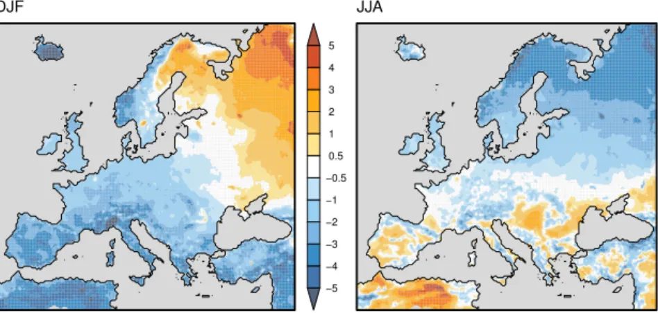
Figure 2 shows the spatial distribution of the daily mean temperature RMIB-UGent-11 BIAS in winter (DJF, left) and summer (JJA, right) for the years inIK14. Compared to Fig. 2 from K14, the spatial bias of RMIB-UGent-11 in winter looks very similar to CNRM-11. Both models show a general cold bias in southern Europe, a warm bias in north-eastern Europe and a large east–west bias gradient linked to orogra-phy in Scandinavia. Compared to CNRM-11, the cold biases in mountainous regions are smaller for RMIB-UGent-11. In summer, again CNRM-11 and RMIB-UGent-11 share some biases although the difference is larger than in winter, and again the orographic forcing of the bias of CNRM-11 is more pronounced. Generally we find a cold bias, except in south-ern Europe where a warm bias is present.
−5 −4 −3 −2 −1 −0.5 0.5 1 2 3 4 5
DJF JJA
Figure 2.Spatial BIAS of near-surface air temperature (K) over the sampleIK14for DJF (left) and JJA (right) for RMIB-UGent-11. Compare to Fig. 2 of Kotlarski et al. (2014).
again for the high-resolution (top) and low-resolution (bot-tom) simulation. When the background colour is white, the RMIB-UGent-11 value ofsj k(IK14)lies within the K14 high-resolution ensemble spread. If the background colour is yel-low, this value lies outside and is “worse” than the other members of the K14 ensemble. “Worse” means that the abso-lute distance from the RMIB-UGent-11 value based onIK14 (top red dash) to the optimal value (grey line) is larger than that of any other K14 ensemble member. For example, the bias for the Iberian Peninsula in winter (in short written as BIAS-IP-DJF) is more negative than any other model, and it is in absolute value the furthest from the optimal 0 K. If in-stead the background colour is green, this indicates again the value is outside of the K14 ensemble but not the furthest from the optimal value. This implies that either RMIB-UGent-11 outperforms all other models (e.g. RSV-AL-DJF) or is not the worst model as defined above (e.g. RSV-EA-DJF is out-side of the K14 ensemble, but not as bad as models at the other end of the ensemble).
Overall, Fig. 3 shows that (i) RMIB-UGent-11 mostly falls within the K14 ensemble (white background colour), (ii) the jackknife confidence intervals are always much smaller than the total spread of the K14 ensemble, except for RIAV and TCOIAV where the intervals often cover half of the ensem-ble spread, (iii) the difference between the RMIB-UGent-11 (top red dash) and RMIB-UGent-44 (bottom red dash) scores is very small considering the total range covered by the en-semble and the calculated jackknife confidence intervals.
A more detailed analysis shows that for BIAS, RMIB-UGent is almost always on the “cold side” of the K14 ensem-ble and even outside of its range on a fairly large amount of occasions. Especially for IP-DJF and SC-MAM, the cold bias is considerable. Also, RMIB-UGent-44 is slightly (∼0.2 K) colder than RMIB-UGent-11, which may be due to re-gridding and the resolution difference. For 95 %-P, RMIB-UGent-11 is the worst model on four occasions among which most notably again are IP-DJF and SC-MAM.
For spatial correlation (PACO) and variability (RSV) RMIB-UGent-11 performs better. Although in K14 these two metrics are plotted on a Taylor diagram, we choose to show them here separately in one figure for clarity and concise-ness. RSV for RMIB-UGent is almost always larger than 1, even where other models show less variability (e.g. ME). In the Alpine region (AL), RMIB-UGent seems to be able to grasp RSV well, but not at the right locations, as shown by the low PACO, especially in DJF. The jackknife confidence intervals are very small here, which indicates that both RSV and PACO produce very robust scores.
For RIAV and TCOIAV, RMIB-UGent again shows ac-ceptable scores, some being outside of the K14 ensemble in a limited amount of cases. More notably, the jackknife con-fidence intervals are relatively large for these scores and this questions the robustness of these metrics. For example, for FR-MAM the TCOIAV based onIK14is 0.6, but the jack-knife confidence interval extends from 0.6 to 0.8, covering all but two other models. For RIAV a similar situation for AL-JJA can be seen.
3.2 Precipitation
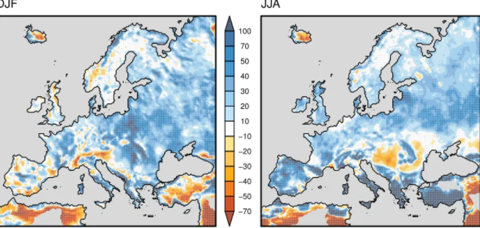
Figure 4 shows the spatial distribution of the relative seasonal precipitation BIAS (in %, (model−observed)/observed) for the winter and summer season for the years inIK14. Com-parison to Fig. 3 of K14 shows that in winter, like all other models, RMIB-UGent-11 generally overestimates precipita-tion amounts, except in northern Africa. In contrast to tem-perature, RMIB-UGent-11 clearly differs from CNRM-11, with the latter showing large dry biases. In summer, RMIB-UGent-11 overestimates precipitation amounts, especially in the Mediterranean. Again, no clear resemblance to CNRM-11 is found.
O. Giot et al.: V alidation of the ALAR O-0 model within the EUR O-CORDEX framew ork Domain BI IP FR ME SC AL MD EA season DJF MAM JJA SON YEAR DJF MAM JJA SON YEAR DJF MAM JJA SON YEAR DJF MAM JJA SON YEAR DJF MAM JJA SON YEAR DJF MAM JJA SON YEAR DJF MAM JJA SON YEAR DJF MAM JJA SON 1 YEAR 1 1 BIAS [K] ●●●● ● ● ●●● ●● ●●● ● ●●● ●● ●●●●●●● ● ● ●●● ● ●●● ● ● ●● ● ● ●●● ●● ● ●● ●●● ● ● ● ●●●●●●● ● ● ● ● ● ● ●● ● ● ● ●● ● ●●● ● ● ● ● ● ● ●●●● ● ● ● ● ● ● ●● ● ● ● ● ● ● ●●●● ● ● ● ● ●●●● ● ● ● ●● ● ●●● ● ● ● ●●● ●●●● ● ●● ●●●●●● ● ● ●● ● ● ●●● ● ● ● ● ● ●●●● ● ● ● ● ● ●●● ● ●● ● ● ●●●●● ●● ● ● ● ●● ● ● ●● ●● ●●● ●● ● ● ●● ● ●●●● ● ● ● ●●●●●● ● ● ●● ●●●● ● ●● ● ● ●● ● ●● ● ● ●●● ●●●● ●● ● ● ● ● ●●● ● ● ● ● ● ● ●●● ● ● ● ●● ●●●● ● ● ● ●● ●● ●● ● ● ● ● ● ● ●●● ● ● ● ● ● ●● ●● ● ● ● ● ● ● ●●● ● ● ● ● ● ● ●●● ●● ● ●●● ●●● ● ● ● ●● ●●●● ● ● ● ● ●●●●● ● ● ● ● ● ● ●● ● ●● ● ●●●●● ● −5 −2 0 2 4
1 95%−P [K] ● ●● ●● ● ● ●● ● ● ●● ● ● ●●● ●●●● ●●●● ● ● ● ●●● ● ● ●● ● ●●●●●●● ● ● ●●●●● ● ●● ● ●● ●● ● ●●● ● ● ● ●● ● ● ● ● ● ● ●●● ●●● ● ●●●●● ● ●● ● ● ●●●●●● ●● ●●●● ●●●● ● ●●● ● ●●●●● ● ● ●●● ● ● ●● ●●● ●●●●● ● ● ● ●●●●●●● ● ● ●● ● ● ●●● ● ● ●● ●●●● ● ●●●●●●●● ● ● ●●●● ● ●●● ●●●● ● ● ●●● ●●●●●●●●● ● ●● ● ●● ● ● ● ● ●●● ●● ●● ● ● ●●●●●● ● ● ●● ●●● ● ● ● ● ● ●●●●● ● ● ● ●●● ● ● ● ● ●● ●●●●● ● ● ● ● ●●●●●● ● ● ● ● ●● ● ●● ●● ● ● ●●● ●● ● ● ● ● ● ● ● ●● ● ● ● ●●●●●●●● ● ●●●●●●●● ● ●● ●●●●●● ● ●●●●●●●● ● ● ● ● ● ●● ● ● ● ● ● ● ●●●● ● ● ● ●● ● ●●● ● ●
0 2 4 6 8 10
1 RSV ●● ● ● ● ● ● ● ● ●● ● ● ● ● ● ● ● ● ● ● ●● ● ● ● ● ● ●●● ● ● ● ● ●● ●●● ● ● ● ●● ● ●●●● ● ● ● ●●● ●● ● ● ● ● ● ● ● ●●● ● ● ● ● ●●●● ● ● ● ●● ●●●● ● ● ●●●●● ●● ● ● ● ●●●●●●● ● ●● ●●●● ● ● ●●●●●● ● ● ● ● ●●●● ● ● ●●●●●● ● ● ● ●● ●●●●● ● ● ●●●● ●● ● ● ●●●●●● ● ● ●●●●●● ● ●●●●● ●●● ● ●●● ● ● ● ● ●● ● ●●●● ● ● ● ● ●●●●●●●● ● ●● ●● ● ●● ● ● ● ● ● ● ●● ● ●●●●●●● ● ● ●●●●● ● ● ● ●●●●●● ● ●●●● ●● ● ● ● ●●● ●●●● ● ● ●●●●● ●● ● ● ●●● ●● ● ● ●●●●●●● ● ● ●●●●●● ● ● ● ● ● ● ●●● ●● ● ●● ● ●● ●● ● ● ● ●●● ● ● ● ● ● ● ● ●●● ●●● ●● ●●●
0 0.5 1 1.5 2
1 PACO ● ● ● ●● ● ●●● ● ●●●● ● ●●● ● ●●●● ● ●●● ● ● ●●● ●●●● ● ● ● ● ● ● ●●● ● ● ●●● ●●●● ● ●●● ● ●●●● ● ● ●● ● ● ●●● ● ● ● ● ● ● ●●● ● ● ● ● ● ● ●●● ● ● ● ● ● ● ●●● ● ● ● ● ● ●● ●● ● ●●●● ● ●●● ● ● ●●● ● ●●● ● ● ● ●● ●●●● ● ●● ●● ● ●●● ● ● ●● ● ● ● ●● ● ● ● ●● ● ●●● ● ● ●●● ● ●●● ● ●● ● ● ● ●●● ● ●● ● ● ● ●●● ● ●● ● ● ● ●●● ● ●● ●●●●● ● ● ●● ● ● ● ●●● ● ● ● ● ● ● ●●● ● ● ● ●● ●●●● ● ● ● ●● ●●●● ● ● ● ● ● ● ●●● ● ● ● ●● ● ●●● ● ● ● ●● ● ●●● ● ● ●●● ● ●●● ● ● ● ● ● ● ●●● ● ● ● ● ● ● ●●● ● ● ● ●● ● ●●● ● ● ●● ● ● ●●● ● ● ● ●● ● ●●● ● ● ●●● ● ●●● ● ● ● ● ● ● ●●● ● ● ●●● ● ●●● ● ●●●● ● ●●●
0.7 0.8 0.9 1
1 RIAV ●●● ●●●●● ● ●● ● ●●●● ● ● ● ● ● ● ●●●● ● ● ● ● ● ● ●●●● ● ● ● ● ●●●●● ● ●●●●●● ● ● ● ● ● ●●●●● ● ● ●● ● ●●●●● ● ● ●● ● ● ●●● ● ●●●●●● ●● ● ● ●●● ●●●● ● ● ●● ● ●●●● ● ● ● ● ● ● ●● ● ● ● ●● ●●●● ● ● ● ●● ● ●● ●● ●● ●● ●●●● ● ●●●● ●●●● ● ● ● ● ● ● ●● ● ● ● ● ● ● ●●●● ● ● ●●●●●●● ● ●●●●● ●● ●● ●●●●● ● ● ● ● ● ● ● ●●●●● ● ●●●● ●●●●● ●●●●● ●●●● ●●● ● ● ●● ●● ● ● ● ●● ● ●● ● ● ● ● ● ● ●● ● ● ● ● ●● ● ●●● ● ● ●●●● ●● ●● ● ●●●●●● ● ● ● ● ●●●●●●● ●● ● ● ● ● ● ● ● ● ●●● ● ● ●●● ● ● ●●● ●●● ● ● ●●●● ●● ●● ●●●● ● ●●●● ●● ●● ● ● ● ● ● ●●● ● ●●● ●● ●● ● ● ●●●●●
0 1 2 3 4
1 TCOIAV ● ● ● ● ● ●● ●● ● ● ●● ● ● ●●● ● ●● ● ●● ● ● ● ● ● ● ● ●●●●● ● ● ● ● ● ●●● ● ●●●● ●●● ●● ● ●●●●● ● ● ● ● ●●● ● ● ● ● ● ● ● ●●●●●● ● ● ● ●● ●● ●● ● ● ●●● ●●●● ● ● ● ● ● ● ● ● ●● ● ●●●●● ● ● ● ● ● ●●● ● ●● ● ● ●●● ●● ●● ● ● ● ●● ● ● ● ●● ● ● ● ● ●● ●● ● ● ● ● ●● ● ● ● ● ● ● ●●● ●● ● ● ● ●● ● ● ● ● ● ● ● ● ●● ● ●● ●● ● ● ●●● ●●●● ● ● ●● ●●● ● ● ● ●●●●●● ●● ● ● ● ● ●● ● ● ● ● ●●●●●● ● ● ● ● ● ●●●●● ● ● ● ● ● ● ● ● ● ● ● ● ●●● ● ● ● ● ● ●● ● ● ● ●● ● ● ● ●● ●●●● ● ● ● ● ● ●●●● ● ● ● ● ●● ● ● ● ● ● ● ● ● ● ● ● ● ● ● ●● ● ● ● ● ● ● ● ●●● ● ● ● ●● ● ● ● ● ●● ● ● ● ● ● ●● ● ● ●● ● ● ● ● ●● ● ●● ● ● ● ● ● ● ● ●●●
0 0.25 0.5 0.75 1
1
1 1 1 1 1 1
K14 models RMIB-UGent (top=.11; bottom=.44)
● ●
Jackknife 95% confidence interval White background: RMIB-UGent is in K14
Green background: RMIB-UGent is not in K14, but better or not the worst Yellow background: RMIB-UGent is not in K14 and the worst
Temperature
Optimal score−70 −50 −40 −30 −20 −10 10 20 30 40 50 70 100
DJF JJA
Figure 4.Spatial BIAS of precipitation (%) over the sampleIK14for DJF (left) and JJA (right) for RMIB-UGent-11. Compare to Fig. 3 of
Kotlarski et al. (2014).
lie within the K14 ensemble, no difference between RMIB-UGent-11 and RMIB-UGent-44 is found and the jackknife confidence intervals are much smaller than the total ensem-ble range except for RIAV and TCOIAV. However, there is a clear absence of yellow scores and an increased presence of green scores, indicating that RMIB-UGent precipitation scores are generally better than the temperature scores.
RMIB-UGent has a wet BIAS for almost all regions and seasons. Remarkably, the best BIAS scores are obtained for SC-MAM and AL-DJF, where large temperature biases were found. Additionally, the corresponding 95 %-P scores are also on the low side which shows that the good performance is not due to compensating biases.
For RSV, RMIB-UGent performs relatively well and for PACO it excels, with 10 out of 80 region–season combina-tions performing better than the complete K14 ensemble. Only for AL-MAM is its performance not satisfactory, but remark that the actual score is an extreme outlier considering the jackknife confidence interval.
For RIAV, RMIB-UGent again performs consistently well, especially compared to the K14 ensemble which sometimes shows a large overestimation of interannual variability, i.e. very large values of RIAV. On the other hand, TCOIAV is mostly on the low side of the K14 ensemble, which shows that although RMIB-UGent gets the variability right, the ac-tual temporal correlation is not well grasped. As for temper-ature, the large jackknife confidence intervals question the robustness of the scores.
4 Discussion
This is the first time ALARO-0 was used for a climate exper-iment. Nevertheless, the performance of ALARO-0 on sea-sonal and yearly scales for both near-surface air tempera-ture and precipitation is satisfactory. Generally ALARO-0 performs well, which is quantified by the large number of white boxes in Figs. 3 and 5 indicating that the ALARO-0
score lies within the existing K14 ensemble. For precipita-tion, ALARO-0 even outperforms all other models on nu-merous occasions. These results are encouraging, given that ALARO-0 does not yet have the experience in climate mod-elling that some of the other models of the K14 ensemble had, but was directly ported from its NWP setup. Although the 12.5 km resolution was also a novelty for the K14 mod-els, their performance undoubtedly benefited from previous optimisations for climate experiments, albeit at a lower reso-lution of 50 km.
Some issues still remain. Most notably, this study has re-vealed some large temperature biases in Scandinavia and eastern Europe. The spatial pattern of the BIAS resembles CNRM’s ARPEGE model (shown in Fig. 2 of K14). In win-ter, the common east–west bias gradient can possibly be at-tributed to the shared dynamical core and the strong synop-tic scale forcing in winter. In NWP applications of the AL-ADIN system similar symptoms have been diagnosed and have been shown to be related to stable boundary layer is-sues. The dampened bias patterns for RMIB-UGent-11 com-pared to CNRM-11 in the Alps and other mountainous re-gions is probably due to the different surface and snow cover scheme that is used by both. In summer, RMIB-UGent-11 is generally cold biased, except in southern Europe where it suffers from the common summer warm bias, probably due to soil moisture feedbacks. Also, the RMIB-UGent-11 and CNRM-11 bias patterns are less alike than in winter, possibly due to the increased number of local processes that influence and feed back into the mean fields. Both spatial and temporal variability are very well reproduced by ALARO-0, while cor-relations are on the low side compared to other models. The latter could partly be explained by the comparatively larger domain of ALARO-0 which could imply a weaker control of the boundary forcing.
al-O. Giot et al.: V alidation of the ALAR O-0 model within the EUR O-CORDEX framew ork Domain BI IP FR ME SC AL MD EA season DJF MAM JJA SON YEAR DJF MAM JJA SON YEAR DJF MAM JJA SON YEAR DJF MAM JJA SON YEAR DJF MAM JJA SON YEAR DJF MAM JJA SON YEAR DJF MAM JJA SON YEAR DJF MAM JJA SON YEAR BIAS [%] ● ●●● ● ● ● ●● ● ●●● ● ● ●●● ●●●● ● ●● ● ● ● ●●● ● ● ●●● ●●●● ● ● ●● ● ● ●●● ● ●●● ● ●●●●●●● ●● ●● ● ●●● ●● ● ●●●●● ●●●● ●●●● ● ● ●●● ●●●● ● ● ●● ● ● ●●● ● ● ●● ● ●●● ● ● ● ●● ● ●●●● ● ● ●●● ●●●● ● ● ●● ● ● ●● ● ● ● ●●● ● ●●● ● ● ●●● ●●●● ● ● ● ● ● ● ●● ● ● ● ●● ● ● ●●● ● ● ●● ● ●● ● ● ● ● ●●● ●● ● ●●●● ●● ●●● ●● ●●● ● ● ●●●● ● ●● ● ●● ● ● ● ●●● ● ● ●● ●● ●●● ● ● ●●● ● ● ●● ● ● ●●●● ● ●●● ● ● ● ●● ● ●● ● ● ●● ●● ● ●● ● ● ● ●●● ●●● ● ● ●●● ● ● ●● ● ●● ●● ● ● ● ● ● ● ●●●● ●●● ● ● ●●● ● ● ● ●● ● ●● ●● ● ● ●● ● ● ● ● ● ● ●● ● ● ●●●● ● ● ● ● ● ●● ●● ● ●● ● ● ●● ● ● ● ● ● ●
−60 0 60 120 180
95%−P [%] ●● ●●●●●●● ● ●● ●●●●●● ●●●●● ●●●● ● ●●●●● ● ● ● ●●●●●●● ●● ●●● ● ● ● ●● ● ● ●●●●●●●● ● ● ● ● ● ●● ● ● ●● ●● ●● ●● ● ● ●● ●●● ●●● ● ●●●● ●●● ● ●●●● ● ●●● ● ● ●●● ●●● ●● ●●●●●● ●●● ●●●●●●● ●● ● ●● ● ● ● ●●● ● ● ● ●● ●●●● ● ●●●●● ●●● ●●● ●● ●●● ● ●●●●●●● ●● ● ●● ● ● ●●●● ● ●● ● ● ● ●●● ● ● ● ●●●● ● ● ●● ● ● ● ●●●● ● ● ● ● ● ● ● ●● ● ●● ●● ●●● ● ● ● ● ●●●●● ● ● ● ●●● ● ● ●● ●●● ●●● ●● ● ● ●●●● ●●● ● ● ●●●● ●●● ● ● ● ● ● ●●●●● ● ●● ● ● ●● ● ● ●●●●●●●● ● ●● ●● ●●●● ● ●● ●● ● ● ●● ● ●● ●●●●●● ● ● ● ● ●●●●● ● ●●● ●●●● ● ● ● ● ●● ● ●●●
0 100 200 300 400
RSV ●●● ●●●●● ● ●● ●●● ●●●● ● ●●●● ●●● ● ●●●●●●●●● ●●● ●●●●●● ●● ● ●●●● ●● ●●● ●● ●● ●● ●●●●●●● ● ● ●●●●●●●●● ● ●● ● ●●●●● ●●●● ●●●●● ● ●●●●●●●● ● ●●● ● ●●●● ●●●●●● ●●● ● ●●●● ●●●● ●●●●●● ●● ● ● ●● ●●●● ●● ● ●●●●●●●● ●●● ●● ●●●● ●●● ●●●●● ● ●●●●●●●●● ●●●● ●●●● ● ● ●● ● ●● ●●● ●●●●● ● ●● ● ●●●● ● ● ●●● ●●●●● ●● ●● ● ● ● ●●●●● ● ● ●● ●● ●●● ● ● ●●●●●●● ● ● ● ● ●● ●●● ● ●● ●●●●●● ● ● ●● ●●● ● ●● ● ● ● ●● ●● ●● ●●●●●●●●● ● ●●●●●●●● ● ●●●● ●●●● ● ●●●● ●●●● ●●● ●● ●●●● ● ●●●●●● ●● ● ●●●●●● ●●
0 1 2 3 4
PACO ● ● ●●●●●●● ● ●●●●●●●● ● ● ● ● ● ● ● ●● ● ● ●● ●● ●●● ● ●●●●●●●● ● ● ●● ● ● ●●● ● ● ●● ● ● ●●● ● ●●● ● ● ●●● ● ● ●● ●● ● ●● ● ●●● ●● ●●● ● ● ● ● ● ● ●●● ● ● ●● ● ● ●●● ● ● ●●● ●● ● ● ● ●●●●●●● ● ● ● ● ● ● ●●● ● ● ●●●● ●●● ● ● ● ● ● ● ● ●● ● ● ● ● ● ● ● ●● ● ●●●● ●●●● ● ● ● ●● ● ●●● ● ●●● ●●●●● ● ● ● ● ● ●●●● ● ●● ● ● ● ●●● ● ●●● ● ●●●● ● ●●● ●●●●● ● ● ●●●●●●● ● ● ●●● ● ●●● ● ● ●● ● ● ●●● ● ● ●● ● ● ● ●● ● ● ●●● ● ●●● ● ●● ● ●● ● ●● ● ● ●● ● ● ●●● ●● ● ● ● ● ●●● ● ●● ● ● ● ●●● ● ●● ● ●● ●●● ● ● ●● ●●●●● ● ●●● ● ● ● ●● ● ● ●● ● ● ● ●● ● ●● ● ● ●● ● ● ● ● ●● ● ● ●●●
0 0.25 0.5 0.75 1
RIAV ● ●● ●● ● ● ●● ● ●● ● ● ● ● ●● ● ●●●● ● ●● ● ●● ● ● ● ● ●● ● ●● ●● ● ●●●● ●●●● ● ●●● ● ● ●●●●●● ●● ●● ● ●● ● ●● ● ●●●● ● ● ●● ● ● ●●● ● ●●● ● ●●●● ● ●●● ● ● ●●● ● ●● ● ● ● ● ●●● ● ● ●● ●●●● ● ● ● ● ● ●●●● ● ● ●● ● ● ● ● ● ● ●●● ● ● ●●●● ● ●● ● ● ● ● ● ● ● ● ● ●●● ●● ● ● ●● ●●● ● ● ● ●● ● ● ●● ●● ● ● ●● ● ● ● ● ● ● ● ●● ● ●● ●●●●● ● ●●●● ● ● ●●● ● ● ● ● ● ● ● ● ● ● ● ● ●● ● ●● ● ● ●● ● ● ● ● ● ● ● ● ● ● ● ● ●● ● ●● ●●● ● ●● ● ●● ●●● ●●● ● ●● ● ● ● ●● ● ● ● ●● ● ● ● ● ● ● ●● ● ● ● ● ● ●● ● ● ● ●● ● ● ● ● ● ● ●● ● ●● ● ● ● ● ● ● ● ●● ●● ● ● ● ● ● ● ●● ● ● ● ● ● ● ●● ● ● ● ●● ● ● ● ● ● ● ● ●●●
0 1 2 3 4
TCOIAV ● ● ●●●●● ● ● ● ●●● ● ●● ● ● ● ●● ●●●● ● ● ● ● ● ●●●● ● ● ● ● ●●●●● ●● ● ● ●● ●● ● ●● ● ● ● ●● ● ● ● ● ● ● ● ● ● ● ● ● ● ● ●● ●● ● ● ● ● ● ● ● ●●● ●● ● ● ● ●●● ●● ●● ●● ● ● ● ● ● ● ● ● ● ● ●●● ● ● ● ● ●● ●●● ●● ● ● ●● ●●●● ● ● ● ●●● ● ● ● ●● ● ● ● ● ● ● ● ● ● ● ● ● ● ●● ●● ● ● ● ● ● ● ● ● ● ● ● ● ● ●● ● ● ● ● ● ● ● ●● ●● ●● ●● ● ● ●● ● ● ● ● ●●●● ● ● ● ● ● ● ● ●●● ● ● ● ● ● ● ●●●● ● ● ● ● ● ●● ●● ● ● ● ● ●● ● ● ●● ● ● ● ●● ● ● ● ● ● ● ● ●●●● ● ● ● ● ●●●● ● ● ● ● ● ● ●●●●● ● ● ● ●●● ● ● ●●● ● ● ● ● ● ● ● ● ● ● ● ●●● ● ● ● ● ● ● ● ●● ●● ● ● ● ● ● ●●●● ● ● ●● ●●●●● ●● ● ● ● ●●● ● ● ● ● ● ● ●●●● ● ● ● ● ● ● ●● ● ● ●
0 0.25 0.5 0.75 1 K14 models RMIB-UGent (top=.11; bottom=.44)
● ●
Optimal score Jackknife 95% confidence interval White background: RMIB-UGent is in K14
Green background: RMIB-UGent is not in K14, but better or not the worst Yellow background: RMIB-UGent is not in K14 and the worst
ways below 50 %. Contrary to temperature, the precipitation bias pattern shows no resemblance to ARPEGE (shown in Fig. 3 of K14). This can be attributed to the different mi-crophysics and convection parameterisation schemes that are used by both models. A similar result was found for the three WRF experiments that were analysed in K14. These only dif-fered in the parameterisation schemes used, but often covered the complete ensemble spread. Remarkably, in Scandinavia all precipitation scores are very good, although temperature scores are sometimes very bad. It is very possible that the two are linked and some compensating effects or feedbacks exist, which is an additional incentive for a more thorough study. The good scores for spatial variability (RSV) and cor-relation (PACO) show that ALARO-0 is capable of produc-ing not only the right amount of precipitation but also at the right locations. The common model overestimation of spatial variability is also present in the RMIB-UGent simulations, but as stated in K14, this could be due to a smoothing of the reference E-OBS data set. Temporal variability is very well reproduced, but correlations are again rather low.
Similarly to the conclusions in K14, no consistent differ-ence between the low- and high-resolution simulations in the scores is shown. However, based on preliminary results, we expect that at the sub-daily scale the timing of precipitation is better represented by the high-resolution simulation.
Finally, it is clear that the periodIK14(1989–2010) used in K14 is sufficient to produce robust scores for BIAS, 95 %-P, RSV, PACO and partly RIAV. This is quantified by the fact that the jackknife intervals for these metrics are very small compared to the total ensemble spread and they therefore do not depend strongly on the period used to compute them. For example, temperature biases calculated forIK14 are mostly within 0.1 K of the jackknife mean. This does not hold for some RIAV and most of the TCOIAV scores due to the fact that these exactly assess interannual variability. For model in-tercomparison a larger period should be considered for these scores.
5 Conclusions
The ALARO-0 model has its origins in the general circula-tion model ARPEGE and mainly its limited area model AL-ADIN. The new microphysics and convection scheme 3MT was implemented in ALADIN to form ALARO-0, which is used operationally for daily weather forecasts at the Royal Meteorological Institute of Belgium (RMIB). In this study, for the first time ever, the ALARO-0 model was used to per-form continuous climate simulations on a European scale for a 32-year period. Within the framework of the CORDEX project, one low- and one high-resolution simulation were done on the EURO-CORDEX domain for the period 1979– 2010, using the ERA-Interim reanalysis as boundary condi-tions. The results are compared to an existing ensemble of 19 similar simulations using different models that were
anal-ysed in Kotlarski et al. (2014), referred to as K14 in this text. One of the models used in K14 is the ARPEGE model by the Centre National de Recherches Météorologiques (CNRM), which, due to its relation to ALARO-0, serves as a first ref-erence for the performed simulations.
The main conclusions are that (1) ALARO-0 is able to rep-resent both seasonal mean near-surface air temperature and accumulated precipitation amounts well and (2) all scores computed in K14 are robust, except for RIAV and TCOIAV.
The first conclusion is founded by the fact that most of the ALARO-0 scores lie within the K14 ensemble, thus not performing worse or better than other models. This is quali-fied in Figs. 3 and 5 by a white background. For temperature, some clear cold biases remain, which will be the subject of a follow-up study. Also, for temperature ALARO-0 seems to share some large biases with ARPEGE, while for precip-itation this is not the case due to the inclusion of the 3MT scheme in ALARO-0. For precipitation, ALARO-0 performs very consistently for all scores, regions and seasons and bet-ter on several instances than all other models in the K14 en-semble.
In the second conclusion, robust means “independent of the time period used to compute the scores”. The RMIB-UGent simulations span the 32-year period 1979–2010, which is longer than the 20-year period 1989–2008 used in K14. By taking 1000 random 20-year samples from the 32-year pool, we computed 95 % confidence intervals for all scores. Figures 3 and 5 show that the confidence intervals (red transparent bands) are generally much smaller than the total ensemble spread. Assuming this also holds for other models, this shows that model differences are significant. For RIAV this does not always hold and a longer period should be taken into account to compute the scores. For TCOIAV the situation is even more problematic and scores or model ranking should not be interpreted too strictly.
The outcomes of this study confirm the potential of ALARO-0 as a climate model on European scales. Fu-ture work will focus on pinpointing the causes of some of the remaining biases and performing simulations in which ALARO-0 is driven by a GCM, rather than ERA-Interim.
Acknowledgements. The computational resources and services used in this work were provided by the VSC (Flemish Super-computer Center), funded by the Hercules Foundation and the Flemish Government – department EWI. This work was financially supported by the Belgian Science Policy (BELSPO) within the ECORISK (SD/RI/06A) and the CORDEX.be (BR/143/A2) projects. We would also like to thank Sven Kotlarski and Klaus Keuler for providing the necessary data and the two anonymous reviewers for their comments and useful suggestions that have improved the manuscript.
References
ALADIN international team: The ALADIN project: Mesoscale modelling seen as a basic tool for weather forecasting and at-mospheric research, WMO Bull., 46, 317–324, 1997.
Chan, S. C., Kendon, E. J., Fowler, H. J., Blenkinsop, S., Roberts, N. M., and Ferro, C. A. T.: The Value of High-Resolution Met Office Regional Climate Models in the Simulation of Mul-tihourly Precipitation Extremes, J. Climate, 27, 6155–6174, doi:10.1175/JCLI-D-13-00723.1, 2014.
Christensen, J. and Christensen, O.: A summary of the PRUDENCE model projections of changes in European climate by the end of this century, Climatic Change, 81, 7–30, doi:10.1007/s10584-006-9210-7, 2007.
Davies, H. C.: A lateral boundary formulation for multi-level prediction models, Q. J. Roy. Meteor. Soc., 102, 405–418, doi:10.1002/qj.49710243210, 1976.
De Meutter, P., Gerard, L., Smet, G., Hamid, K., Hamdi, R., De-grauwe, D., and Termonia, P.: Predicting Small-Scale, Short-Lived Downbursts: Case Study with the NWP Limited-Area ALARO Model for the Pukkelpop Thunderstorm, Mon. Weather Rev., 143, 742–756, doi:10.1175/MWR-D-14-00290.1, 2015. De Troch, R., Hamdi, R., Van de Vyver, H., Geleyn, J.-F., and
Termonia, P.: Multiscale Performance of the ALARO-0 Model for Simulating Extreme Summer Precipitation Climatology in Belgium, J. Climate, 26, 8895–8915, doi:10.1175/JCLI-D-12-00844.1, 2013.
Dee, D. P., Uppala, S. M., Simmons, A. J., Berrisford, P., Poli, P., Kobayashi, S., Andrae, U., Balmaseda, M. A., Balsamo, G., Bauer, P., Bechtold, P., Beljaars, A. C. M., van de Berg, L., Bid-lot, J., Bormann, N., Delsol, C., Dragani, R., Fuentes, M., Geer, A. J., Haimberger, L., Healy, S. B., Hersbach, H., Hólm, E. V., Isaksen, L., Kållberg, P., Köhler, M., Matricardi, M., McNally, A. P., Monge-Sanz, B. M., Morcrette, J.-J., Park, B.-K., Peubey, C., de Rosnay, P., Tavolato, C., Thépaut, J.-N., and Vitart, F.: The ERA-Interim reanalysis: configuration and performance of the data assimilation system, Q. J. Roy. Meteor. Soc., 137, 553–597, doi:10.1002/qj.828, 2011.
Dudhia, J.: A history of mesoscale model development, Asia-Pac. J. Atmos. Sci., 50, 121–131, doi:10.1007/s13143-014-0031-8, 2014.
Gerard, L.: An integrated package for subgrid convection, clouds and precipitation compatible with the meso-gamma scales, Q. J. Roy. Meteor. Soc., 133, 711–730, 2007.
Gerard, L. and Geleyn, J.-F.: Evolution of a subgrid deep convection parameterization in a limited area model with increasing resolu-tion, Q. J. Roy. Meteor. Soc., 131, 2293–2312, 2005.
Gerard, L., Piriou, J.-M., Brožková, R., Geleyn, J.-F., and Banciu, D.: Cloud and precipitation parameterization in a meso-gamma-scale operational weather prediction model, Mon. Weather Rev., 137, 3960–3977, 2009.
Giorgi, F. and Mearns, L. O.: Introduction to special section: Re-gional Climate Modeling Revisited, J. Geophys. Res.-Atmos., 104, 6335–6352, doi:10.1029/98JD02072, 1999.
Giorgi, F., Jones, C., and Asrar, G. R.: Addressing climate informa-tion needs at the regional level: the CORDEX framework, WMO Bulletin, 58, 175–183, 2009.
Hamdi, R., Giot, O., Troch, R. D., Deckmyn, A., and Termo-nia, P.: Future climate of Brussels and Paris for the 2050s under the {A1B} scenario, Urban Climate, 12, 160–182, doi:10.1016/j.uclim.2015.03.003, 2015.
Haylock, M. R., Hofstra, N., Klein Tank, A. M. G., Klok, E. J., Jones, P. D., and New, M.: A European daily high-resolution gridded data set of surface temperature and precipi-tation for 1950–2006, J. Geophys. Res.-Atmos., 113, D20119, doi:10.1029/2008JD010201, 2008.
Hohenegger, C., Brockhaus, P., and Schär, C.: Towards climate sim-ulations at cloud-resolving scales, Meteorol. Z., 17, 383–394, doi:10.1127/0941-2948/2008/0303, 2008.
IPCC: Summary for Policymakers, book section SPM, 1–30, Cam-bridge University Press, CamCam-bridge, United Kingdom and New York, NY, USA, doi:10.1017/CBO9781107415324.004, 2013. Kendon, E. J., Roberts, N. M., Senior, C. A., and Roberts, M. J.:
Realism of Rainfall in a Very High-Resolution Regional Cli-mate Model, J. CliCli-mate, 25, 5791–5806, doi:10.1175/JCLI-D-11-00562.1, 2012.
Kotlarski, S., Keuler, K., Christensen, O. B., Colette, A., Déqué, M., Gobiet, A., Goergen, K., Jacob, D., Lüthi, D., van Meij-gaard, E., Nikulin, G., Schär, C., Teichmann, C., Vautard, R., Warrach-Sagi, K., and Wulfmeyer, V.: Regional climate model-ing on European scales: a joint standard evaluation of the EURO-CORDEX RCM ensemble, Geosci. Model Dev., 7, 1297–1333, doi:10.5194/gmd-7-1297-2014, 2014.
Lin, J.-L., Qian, T., and Shinoda, T.: Stratocumulus Clouds in Southeastern Pacific Simulated by Eight CMIP5-CFMIP Global Climate Models, J. Climate, 27, 3000–3022, doi:10.1175/JCLI-D-13-00376.1, 2014.
Spiridonov, V., Déqué, M., and Somot, S.: ALADIN-CLIMATE: from the origins to present date, ALADIN Newsletter, 29, 89– 92, 2005.
Sun, D.-Z., Yu, Y., and Zhang, T.: Tropical Water Vapor and Cloud Feedbacks in Climate Models: A Further Assess-ment Using Coupled Simulations, J. Climate, 22, 1287–1304, doi:10.1175/2008JCLI2267.1, 2009.
Taylor, K. E., Stouffer, R. J., and Meehl, G. A.: An Overview of CMIP5 and the Experiment Design, B. Am. Meteorol. Soc., 93, 485–498, doi:10.1175/BAMS-D-11-00094.1, 2011.
Teutschbein, C. and Seibert, J.: Regional Climate Models for Hy-drological Impact Studies at the Catchment Scale: A Review of Recent Modeling Strategies, Geography Compass, 4, 834–860, doi:10.1111/j.1749-8198.2010.00357.x, 2010.