Faculty of Economics, Administration and Accounting Department of Economics
Postgraduate Program in Economic Theory
Impacto de operações de venda a descoberto na eficiência de mercado The impact of short selling on market efficiency
Daniel Dantas de Castro
Supervisor: Prof. Dr. Bruno Cara Giovannetti
Reitor da Universidade de São Paulo
Prof. Dr. Adalberto Américo Fischmann
Diretor da Faculdade de Economia, Administração e Contabilidade
Prof. Dr. Hélio Nogueira da Cruz Chefe do Departamento de Economia
Prof. Dr. Márcio Issao Nakane
Impacto de operações de venda a descoberto na eficiência de mercado The impact of short selling on market efficiency
Dissertação apresentada ao Programa de Pó Graduação em Economia do Departamento de Economia da Faculdade de Economia, Ad-ministração e Contabilidade da Universidade de São Paulo, como requisito parcial para a obtenção do título de Mestre em Ciências.
Orientador: Prof. Dr. Bruno Cara Giovannetti
Versão Corrigida
(versão original disponível na Faculdade de Economia, Administração e Contabilidade)
FICHA CATALOGRÁFICA
Elaborada pela Seção de Processamento Técnico do SBD/FEA/USP
Castro, Daniel Dantas de.
Impacto das operações de venda a descoberto na eficiência do mercado / Daniel Dantas de Castro. -- São Paulo, 2015.
44 p.
Dissertação (Mestrado) – Universidade de São Paulo, 2015. Orientador: Bruno Cara Giovannetti.
1. Finanças - Brasil. 2. Mercado financeiro. 3. Transferência de ações. I. Universidade de São Paulo. Faculdade de Economia, Administração e Contabilidade. II. Título.
Esta dissertação estuda os impactos da restrição à venda a descoberto na eficiência de preço dos ativos negociados em bolsa. O estudo utiliza uma base de dados com todos os negócios de aluguel de ação realizados no Brasil entre janeiro de 2009 e julho de 2011, bem como séries de preços em alta e baixa frequência para o cálculo dos índices de eficiência de preço.
As principais descobertas incluem o mapeamento das características de ações eficientes (mais líquidas, empresas maiores e maior book-to-market); a evidência de um prêmio de risco a ser pago ao investidor que mantém ações menos eficientes em sua carteira; a relação positiva entre eficiência de preço e venda a descoberto e o estudo de caso da "barriga de aluguel", onde verifica-se, pelo aumento da restrição às operações de venda a descoberto, um aumento da ineficiência de preço ao redor de datas de pagamento de juros sobre o capital próprio.
This article studies how short-sale constraints affect price efficiency in Brazilian stocks. The study uses a data set with all equity loan deals done in Brazil between January 2009 and July 2011.
The main findings are the mapping of efficiency stock characteristics (i.e. stocks with more liquidity, larger size and greater book-to-market); an evidence of efficiency risk premium paid for investors that keep price-inefficient stocks in their portfolio; a positive relation between short selling and price efficiency and the event study of tax arbitrage, where it’s possible to check that price inefficiency is positively related to short selling during the payment of interest on net equity.
1 Introduction . . . 1
2 Lending equity and its literature . . . 3
3 Data and samples . . . 7
4 Price efficiency index. . . 8
4.1 Low frequency efficiency indexes . . . 8
4.2 High frequency efficiency indexes . . . 10
5 Empirical results . . . 12
5.1 Exercises with low frequency indexes . . . 12
5.1.1 Stock portfolio and efficiency . . . 12
5.1.2 Efficency as a risk factor . . . 13
5.1.3 Loan fee and price efficiency indexes . . . 14
5.2 High frequency indexes exercises . . . 15
5.2.1 Event study of tax arbitrage . . . 15
6 Conclusion . . . 19
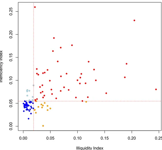
Figure 1 – Relation between illiquidity and inefficiency measures . . . 26 Figure 2 – Event Study - Loan fee around interest on net equity payment . . . . 28 Figure 3 – Event Study - Lended equity quantity around interest on net equity
payment . . . 28 Figure 4 – Event Study - Loan fee around dividend payment . . . 29 Figure 5 – Event Study - Lended equity quantity around dividends payment . . 29 Figure 6 – Loan fee (left axis) and pricing error (right axis) - Closing values from
intraday intervals of 15 minutes . . . 30 Figure 7 – Loan fee (left axis) and |��30| (right axis) - Closing values from
intraday intervals of 30 minutes . . . 31 Figure 8 – Loan fee (left axis) and |��30| (right axis) - Average values between
opening and closing from intraday intervals of 30 minutes. . . 32 Figure 9 – Loan fee (left axis) and |��15| (right axis) - Average values between
opening and closing from intraday intervals of 15 minutes. . . 33 Figure 10 – Robustness Check - Dividend Event - Loan fee (left axis) and |��30|
Table 1 – Correlation between low frequency efficiency metrics . . . 23 Table 2 – Efficiency portfolio characteristics from 2001 to 2014 . . . 24 Table 3 – Efficiency sorted portfolios - Regression results . . . 25 Table 4 – Impacts of short selling constraints on price efficiency - Low Frequency
Analysis . . . 27 Table 5 – Mean test around interest on net equity payment date - High Frequency
1 Introduction
This study is about the impacts of short selling over price efficiency of stocks traded in Brazilian stock exchange market. To give base to this discussion this paper starts co-relating efficiency and other stock characteristics. There have been evidences that stocks with more efficient prices have more liquidity and belong to bigger companies with a higher trading volume than companies with less efficient prices.
Proceeding to an efficiency study between portfolios, there were evidences of the existence of a risk premium paid to investors that maintain less efficient stocks in their portfolios.
After an efficiency analysis, this paper links such concept with short selling. The results show that portfolios in which such deals are more constrained have, in average, inefficient prices.
An event study analyzes the opportunity of fiscal arbitrage called by Brazilians traders as “barriga de aluguel”, that poses an external constraint on stock lending market in reason of interest on net equity (IoNE) payment. As in Bonomo et al. [2015], this event is used as a quasi-natural experiment to address endogeneity problems. As result, it is noticeable that short selling constraints are associated with an increase in price inefficiency throughout the IoNE date, which is the last day to buy the stock and qualify to receive the interest on net equity.
In synthesis, the conclusion of this paper is that short selling has a positive effect on market efficiency. The constraint of such deals results in prices being even more distant from their fundamentals.
The motivation to undertake this study came through the importance of equity lend in market deals and the theme divergence found in financial literature.
Stock lending deals generate great amount of resources. Official data from BM&FBOVESPA [2015] shows that in 2014 R$735 billion came through stock lend in over 1.5 million deals, which stands for about 42% of a R$1.73 trillion market volume. Deals had a monthly average of 290 distinct stocks.
All stocks listed at BM&FBOVESPA are eligible to be lend and all deals are made and, necessarily, registered at BM&FBOVESPA1
. Brokers insert orders (for lending or renting) electronically so that deals can be done. There is also the possibility of an operation where the broker already knows both counterparts and only registers the deal
1
over the counter at BM&FBOVESPA.
According to Boehmer and Wu[2012], the economic theory has divergent points of view about the consequences of short selling on price discovery or, generically, on market quality. In some models the agents that do such deals are well informed, they promote efficiency taking badly priced stocks to values closer to their fundamentals [Diamond and Verrecchia, 1987]. In other models, some stock borrowers follow manipulative and predatory trade strategies that result in less informative prices [Goldstein and Guembel, 2008] or cause overshooting [Brunnermeier and Pedersen,2005].
The impact of short selling constraint is still a theme discussed these days, as it will be seen there are many more articles published in finance literature about it.
2 Lending equity and its literature
One of the options available for an investor who anxiously waits for a decrease in the value of stocks traded in the market is to sell them: the agent sells at time � to rebuy it at �+�, for a lower price, rebuilding the original portfolio and making profit by the price variation.
Even though the agent does not have the stocks that he desires to sell in his portfolio, with short selling it becomes possible: agents can get there desired stocks trough a lend contract where the borrower will become, to legal matters, the stock-owner, agreeing return it to the lender until the specified date together with the settlement fee.
Stock lending deals generate great amount of resources. Official data from BM&FBOVESPA [2015] shows that in 2014 R$735 billion came through stock lend in over 1.5 million deals, which stands for about 42% of a R$1.73 trillion market volume. Deals had a monthly average of 290 distinct stocks.
All stocks listed at BM&FBOVESPA are eligible to be lend and all deals are made and, necessarily, registered at BM&FBOVESPA1
. Brokers insert orders (for lending or renting) electronically so that deals can be done. There is also the possibility of an operation where the broker already knows both counterparts and only registers the deal over the counter at BM&FBOVESPA.
It is interesting to notice that there is a slight difference between equity lending and short selling. Equity lending is a deal registered in the stock market where a stock borrower and lender set contract terms such as: underlying asset, deadline and fee rate. this is where short selling starts, but not all equity lending contracts result in short selling. For this to happen the borrower needs to sell the borrowed equities on the spot market what not always occurs, as shown in the tax arbitrage event. Thus, not all the equity lending implies a short selling.
According to Boehmer and Wu[2012], the economic theory has divergent points of view about the consequences of short selling on price discovery or, generically, on market quality. In some models the agents that do such deals are well informed, they promote efficiency taking badly priced stocks to values closer to their fundamentals [Diamond and Verrecchia, 1987]. In other models, some stock borrowers follow manipulative and predatory trade strategies that result in less informative prices [Goldstein and Guembel, 2008] or cause overshooting [Brunnermeier and Pedersen,2005].
1
Bai et al.[2006] study the impact of constraints on equity lending in stock pricing and market efficiency. For that purpose, they build a general equilibrium model with two types of agents: those who negotiate to share risks and those who speculate based on private information. Among the main conclusions is the one, where the authors verify that limitations of equity lending to those agents that possess private information can increase market uncertainty (price no longer reflects available information) what could generate an abrupt drop of stock price with raise in volatility.
Beyond theoretical analysis, empirical analysis show interesting results.
Using a database with all equity lending deals done in Brazil from January 2009 to July 2011, Chague et al. [2014b] verified the effects of short selling constraints in stock prices. The authors tested two hypothesis with the information about real alterations on the equity lending offer curve: (i) if equity lending constraints cause overpricing of underlying asset and (ii) if such effect is growing with the increase dispersal opinions among investors. The results confirmed both hypothesis and, are maintained despite variations on the specified proposals.
With the same database,Chague et al. [2013] showed evidences that agents who use equity lending can forecast the drop of a taken stock price within a short term. After that, the investors were classified by type, noticing that private and institutional investors2 were able to anticipate future earnings, differently from foreign investors. The magnitude for such prediction is five times bigger in individual investors than in institutions. In an event study, it is noticed that equity lending operations performed by individual investors have a higher than normal activity on days prior to the announcement of a negative fact. This may show the use of privileged information by those investors inside Brazilian market.
In another article, Chague et al. [2014a] concluded that agents executing equity lending deals are informed, although it is not possible for them do lend the desired quantity, due to the constraints on the limits of tradings3
. The constrained stock price does not reflect the entire information on the market.
The relation between stock returns and short selling is subjected to an endogeneity problem. Bonomo et al. [2015] discuss that and point out the strategies used in literature to address this issue. The authors use the tax arbitrage event as an exogenous natural experiment4
and show that variation of rental fee induced by tax arbitrage operation (a source of short selling constraint) has a positive and large impact on abnormal returns.
2
According to authors, the last case is contrary to evidences obtained from American market
3
Trading limit is established by BM&FBOVESPA.
4
One way of analyzing the impact of short selling on the market is through efficiency index. This was the method used by Saffi and Sigurdsson [2011] for a stock panel of 26 countries. Initially a variety of efficiency indexes have been calculated for those stocks, then the efficiency indexes (dependent variable) were regressed against lending offers and contract fee rates (explainable variables), they are treated as proxies for stock lending constraint, and controlled by variables such as execution costs, liquidity, company size, turnover and so on. This is followed by the analysis of significance and coefficient magnitude.
The efficiency index analysis, based on econometric test made by the authors, lead to the conclusion that a higher level of equity lending offers (less short selling constraint) is associated with an increase in the speed of how information is incorporated to prices and, consequently, on the price efficiency of stocks.
With data from the United States and taking into consideration efficiency indexes, Boehmer and Wu[2012], analogously, find evidences that a higher volume of equity lending (or less short selling constraints) is associated with a higher informational efficiency of prices. In other words, the information is quickly incorporated to prices when short selling is more active. The results don’t show evidences that such operations manipulate the market or destabilize prices.
Efficiency indexes used by those authors can be divided into high and low frequency. High frequency indexes are built with information coming from tradings in the spot market, and then they are used to measure the relative informational efficiency of prices, according to the methodology ofHasbrouck[1993] andBoehmer and Kelley[2009]. The low frequency indexes, based on daily and weekly returns5
of stocks on spot market, make it possible to try out the speed to which public information is incorporated to prices. Those indexes were calculated as established by Hou and Moskowitz [2005].
Boehmer and Wu [2012] carried out analysis to check if there are more equity lending deals on days where extremely negative returns are lately reversed, which could indicates its speculative effect. The results found do not indicate a predatory effect of these deals when market is falling.
Aitken et al. [1998] investigate short selling on a high frequency basis for a market setting in which information on short trades is transparent just after execution. The authors find that short selling are almost instantaneously bad news: the mean reassessment of stock value following short sales is up to -0.2% with adverse information impounded within fifteen minutes or twenty trades. In most markets, however, traders can not identify a short selling operation done in spot market.
5
International literature has recently turned their focus to the effects of short selling constraint in firm real decisions, going beyond the financial concept of price efficiency. Massa et al. [2014] test if short selling has a disciplinary role for firm managers, which implies in a reduction of earning management6
. As a result, the authors have documented a negative relation between these variables and they reinforce that short selling has an external governance effect controlling managers. Using the same principle, Grullon et al. [2015] considered the period when short selling was banned in the United States in order to verify if such constraint has had an impact on firm decision making. The authors found that the ban end caused a decrease on stock prices, issued shares and investments, especially on small firms. This effect links short selling to the real side of economy. The authors associated this decrease on stock prices to a rise in price efficiency in that period.
As shown, the international literature indicates a positive relation of short selling and price efficiency, however its data does not reflect the totality of trades done with equity lending, once relevant markets, such as the U.S., have a decentralized market. Regarding the Brazilian market, where there is a centralization of deals, it is possible to find evidences that short sellers are informed agents and that the tax arbitrage event, in which short sellers are exogenously constrained, generates abnormal stock returns. For the Brazilian market, academic papers showing the relationship between short selling and price efficiency are yet unknown.
6
3 Data and samples
This section exposes the database used in this paper.
Equity lending database
This database contains data from daily deals of equity lending registered in BM&FBOVESPA system. It represents the totality of deals made in the Brazilian market from January 2009 to July 2011.
For each deal, there is information about underlying asset, number of traded stocks, equity lending fee and commission paid by lenders and borrowers. The type of borrower is also available. The main types are funds (mutual or hedge), foreign investors, pension funds and individual investors. It is also possible to differentiate over-the-counter deals.
Database to calculate efficiency indexes
To calculate the efficiency indexes of stock, two price databases were created. The first one has the daily closing price already adjusted by the earnings1
of stocks traded at BM&FBOVESPA from 2000 to 2014, as well as daily volume of trades. With this data the low frequency indexes described in the section 4 were calculated. The second price database, used to calculate high frequency indexes, contains closing, opening, maximum and minimum prices of each stock at 15 minutes intervals2
. Through this way, daily price in high frequency from January 2009 to July 2011 were made available. Other stock information such as book/market value and outstanding stocks came from Economática
data base.
Earnings database
This paper also uses a database with all the payment dates of stock earnings from January 2009 to July 2011. This database contains information about announcement and in-dividends date3
, stock, value and the kind of earnings paid (dividend or interest on net equity).
1
Dividends, interest on net equity, subscription, bonus stock, split, inplit.
2
In this case, around 32 observations a dayper ticker.
3
4 Price efficiency index
The efficiency analysis is done based on indexes available in literature. Below, there is a description of their methodology.
4.1
Low frequency efficiency indexes
The low frequency efficiency indexes of prices generally follow what is stated on the Finance literature1
which considers the returns of stocks traded in open market as something unpredictable.
As defined byFama[1970], if weak efficiency is valid, future price is not determined by information included in its time series, in other words, past price variations do not allow any implication about future return movements. In this case, the less predictable the stock return is, the more efficient its price will be. One way of analyzing price efficiency of a stock is to verify the speed in which the information available to agents is fully incorporated into stock prices. A stock whose information is promptly incorporated has a more informative price and, consequently, is more efficient.
Statistically, it is possible to model efficient prices as a random walk2
. In this specification, the weak efficiency is fully satisfied in a simple way. Overall, efficiency indexes are metrics that quantify how distant the return of a stock is from a white noise.
Cross-correlation ︀
�Cross︀
This efficiency index correlates stock returns and lagged returns of a market index. Once market lagged returns contain information already available to agents, it’s expected of an efficient stock to have already incorporated those information in its price, which means that its returns at time � shouldn’t be affected by lagged market returns. The contemporary correlation exists, but once information is promoted and assimilated by agents, it should disappear completely.
�Cross=����(�i,tw, �m,t−1w)
EfficIndex=���︀�Cross︀
With:
�i,tw, weekly return in time� of stock�;
�m,t−1w, weekly return in �−1of local Market index.
1
SeeHasbrouck[1993], Hou and Moskowitz[2005], and Boehmer and Wu[2012].
2
The more efficient the price is, the closer to zero the index will be.
First order autocorrelation (�1
)
This index correlates stock return and it own one period lagged return (first order autocorrelation). Again, the closer to zero this correlation is, the more efficient the price, based on the same reasons listed in the previous index. News that influence a stock return should be incorporated instantly on prices. A delay, even for one period, generates the possibility of arbitrage and prediction of returns. Furthermore, the absence of first order autocorrelation is a direct statistical result of the hypothesis that return behaves as a white noise.
�1 =����(�i,tw, �i,t−1w)
EfficIndex =���︀
�1︀
With:
�i,tw, weekly return in� of stock�;
�i,t−1w, weekly return in �−1 of stock�.
The more efficient the price is, the closer to zero the index will be.
Low-frequency informational efficiency: R2 ratio (�1)
For this index, the stock daily returns are regressed on market returns and its lags. For a price efficient stock, it is expected just a little contribution of market lags to the explanatory power of regression, measured by �2
.
�i,t =�i+�i�m,t+
5
︁
n=1
�i,−n�m,t−n+�i,t (4.1)
�i,t =�i+�i�m,t+�i,t (4.2)
With:
�i,t, daily return of stock � in time�;
�m,t, daily return of local market index in �;
�m,t−n, daily return of local market index lagged by � periods;
(4.1), unrestricted model; (4.2), restricted model.
The efficiency index is given by: �1i = 1− R2
Restricted
R2
U nrestricted
The more efficient the price is, the closer to zero the index will be.
Using equations (4.1) and (4.2), this index analyzes the magnitude of regression coefficients; even if lagged variables add explanatory power, it is expected for contemporaneous returns to have a bigger impact than lagged ones (�i,−n should not be significantly different from
zero if price is a random walk).
�2i =
︀5
n=1|�i,−n|
|�i|+ ︀5
n=1|�i,−n|
With:
�, lagged period of market returns;
�i,−n, coefficient of lagged market returns in relation to return of the stock �; �i, coefficient of actual market return.
The more efficient the price is, the closer to zero the index will be.
The four price efficiency indexes calculated have also shown a positive correlation and, in many cases, a high one. This indicates that indexes are not divergent in identifying efficient stocks. As each index is unique, calculated according to a particular methodology and with no perfect correlation between them, there is an indication that each index collects a particular aspect of price efficiency (market correlation, autocorrelation, explanatory power and coefficient magnitude). Index correlations are described on table 1.
4.2
High frequency efficiency indexes
Pricing Error: σ2
s
σ2
p
To calculate pricing error, it is assumed that stock prices can be described as an ARIMA(p,1,q) model with drift:
�t =�t−1+�+
∞ ︁
j=0
�j�t−j (4.3)
With:
�t, stock price in�; �, drift;
�t−j, residual value lagged by� periods.
Hasbrouck [1993] assumes that the observed price of a deal done in time �, �t, can
be decomposed in an efficient part, �t, and in an error of price estimation, �t, as shown
next equation:
Using the decomposition of Beveridge and Nelson [1981], there is:
�t=�t+�t (4.4)
�t=�t−1+�+�(1)�t (4.5)
�t=�
∗
(�)�t =� ∗
0�t+� ∗
1�t−1+� ∗
2�t−2+� ∗
3�t−3+... (4.6)
For this purpose, it’s used:
�∗
0 = 1, �(1) =
∞ ︁
j=0
�j, �
∗ k=−
∞ ︁
j=k+1
�j
It is easy to see that through the combination of (4.4), (4.5) and (4.6), equation (4.3) is rebuilt3
.
Price decomposition has interesting properties: (i) The permanent component(�t)
is a random walk that satisfies the concept of weak efficiency seen on Fama [1970]; (ii) The cyclic component(�t)carries everything that deviates the stock price from its efficient
component, that is the reason of the name pricing error; (iii) The bigger thepricing error
is, higher the price inefficiency will be; (iv) Once pricing error mean does not contribute to discussion4
, the variance (�2
s) is calculated and, to compare the index among diverse
stocks available in the market, authors use the ratio between pricing error variance and stock variance, σs2
σ2
p, as the efficiency index; (v) in this conditions, pricing error is inversely proportional to price efficiency; the lower the index is, more efficient the stock price will be.
In the original article, the authors had a database with the prices of each stock transaction. Here, only values taken at a 15 minutes intervals were used. It may differ from the original paper, on the other hand, it demands less computing capacity to be handled with.
Autocorrelation: |��30|
High frequency efficiency index |��30| were calculated for each stock as the absolute value of first order autocorrelation at a 30 minutes interval. Using this metric Boehmer and Wu [2012] shown that their results were qualitatively identical to autocorrelations calculated at 5 and/or 10 minutes intervals.
Since the database have granularity of 15 minutes, the |��30| and |��15| were calculated with closing and opening prices and the simple mean between closing and opening price at the interval.
3
Proof could be checked at page 115 ofCochrane [1997]
4
5 Empirical results
5.1
Exercises with low frequency indexes
5.1.1
Stock portfolio and efficiency
To better understand what is behind price efficiency and to map common charac-teristics between efficient and inefficient stocks, the follow exercise has been done: (i) it is calculated efficiency index of stocks in a particular year �; with these values, the stocks are ranked; (iii) stocks are then divided into quartiles by its efficiency index; each quartile becomes a portfolio (P1, P2, P3 and P4), being P1 composed of stocks of the most efficient quartile and P4 of stocks from the less efficient quartile1
; (iv) these portfolios are kept from the first to the last working day of the year �+ 1; (v) at the beginning of �+ 2, the portfolios are rebalanced based on indexes calculated over the period �+ 1. The process is taken over until the end of the sample (2014).
As a result, P1 is a portfolio that reflects the return of the most efficient stocks traded in BM&FBOVESPA and P4 is the portfolio made by the less efficient ones. This study is about similarities and differences among those portfolios.
Table 2 shows average values per year of diverse metrics for each portfolio. Sys-tematically, P1 stocks (more efficient) are more liquid2
than P4 stocks, indicating that efficiency and liquidity follow the same direction. There is an illiquidity peak in 2008 and 2009, reflecting directly the financial crisis of that period. In those years specifically, the entire market gets more illiquid and the difference of liquidity between P1 and P4 rises.
P4 (less efficient) shows a smaller value of Book-to-Market (Book firm value over Market firm value) if compared to P1 (more efficient). It indicates a positive correlation between stocks value and efficiency. In a moment of crises, when all stocks lose market value (becoming more growth), the book-to-market ratio difference between portfolios was significantly reduced.
The quantity of deals increases year after year, indicating a market trend. Efficient stocks are most heavily traded. This analysis, however, can be mistaken for liquidity analysis as such effects cannot be detached in the table shown.
The growth of market value and traded volume are affected by inflation of the period once these are nominal variables. Yet it is noticeable the consistent difference between the values of P1 and P4 over the years: efficiency is linked to higher market value
1
In this manner, each portfolio has the same number of stocks in its composition. Stocks were equally weighted for portfolio construction.
2
and larger traded volume.
5.1.2
Efficency as a risk factor
Beyond classics SMB, HML, Momentum, and so on, Harvey et al. [2014] do an interesting revision of risk factors found in asset pricing literature. The authors document until April, 2014, 312 alleged idiosyncratic risk factors described in articles and working papers. If there are so many risk factors, will price efficiency also be one? This idea is developed afterwards.
Take two stocks with different price efficiency, but everything else the same. The demanded return between them should be distinct: agents require a higher expected return for the less efficient stock once, with it, there is the risk of having a stock with a less informative price in his investment portfolio, which means, with a price detached from the fundamentals of the company or, in general, that does not reflects all information available in market. This higher expected return is a compensation for the risk of efficiency taken by such agent3
.
Based on such hypothesis, the excess of return of each efficient sorted portfolio was regressed4
on risk factors already documented in literature5
. Results were also reported to portfolio P4-P1, which is a zero cost long-short strategy: P4 portfolio is bought and P1 portfolio is short sold6
, it captures the difference of efficiency between stocks available on market.
The full model is described as follows:
�ei,t =�+�1�m,te +�2�SM B,t+�3�HM L,t+�4�W M L,t+�5�IM L,t+�t (5.1)
With:
�e
i,t is the excess return of the portfolio �;
�e
m,t is the excess return of market portfolio; �t is an error term;
� indexes time;
�SM B,t is the return of a zero cost portfolio bought in small companies and sold in bigger
ones;
�HM L,t is the return of a zero cost portfolio bought in companies with high Book-to-market
and sold in companies with low Book-to-Market;
3
This could be the reason for abnormal returns documented in [Bonomo et al.,2015].
4
The excess of return is calculated by taking the risk free return of portfolios returns.
5
The three Fama and French factors were used (market excess return, SMB and HML), plus momentum and illiquidity. All factors are available onhttp://www.nefin.com.br.
6
�W M L,t is the return of a zero cost portfolio bought in winner companies, which are stocks
that have shown the highest return in the last year and, sold in loser companies, whose stocks have shown the lowest return in the same period and
�IM L,t is the return of a zero cost portfolio bought in illiquid companies and sold in liquid
companies.
Results are presented on table 37
. The reported coefficients are consistent with the analysis done in section 5.1.1, and should be interpreted as follows: suppose an 1 bps exogenous raise in small firm returns, it must raise each portfolio return based on their SMB beta which means that P4 return will raise 0.37 bps in average, on the other hand P1 will raise 0.18 bps. This result leads to conclusion that P4 has smaller firms than P1 (once it will have a higher benefit from the shock).
Using the same interpretation, it is found that more efficient portfolios have a smaller risk SMB (P1 is made of bigger stocks) and IML (P1 is made of more liquid stocks); and bigger HML risk (P1 is made of stocks with larger Book-to-market). When analyzing momentum coefficient (WML), it appear to be lower in P1 than in P4: while the more efficient portfolio (P1) is composed of stocks with a lower return on last year, in P4 there is a balanced proportion between winners and losers, in average.
Alphas (constant term) of P3 and P4 regressions are significantly different from zero. This shows an extraordinary gain controlled by the main risk factors of literature, what may indicate the existence of a risk premium linked to the efficiency of stocks kept on portfolio: price efficiency might be itself a relevant risk factor.
5.1.3
Loan fee and price efficiency indexes
To try to quantify the impact of short selling constraint on price efficiency, some regressions were made using the following panel data model:
�� � �����i,t =�0+�1����� ��i,t+��i,t +�i+�t+�t (5.2)
With:
�� � �����i,t is the low frequency efficiency indexes(�1 or �2)calculated to stock �in
month �;
����� ��i,t is the mean fee of equity lending, used as proxy for short selling constraint;
�i,t are control variables, such as company Size, Book to Market, Free Float ratio regarding
firm characteristics; number of days in a month that the stock was not traded (���0) and Illiquidity index calculated as in Acharya and Pedersen [2004], which controls for stock
7
illiquidity; and a dummy that assumes value 1 if there has been a payment of interest on net equity in that month and
�i and �t are fixed effects of stock and month, respectively.
All variables were standarized to have zero mean and standard deviation of 1.
The results can be seen on table4. It is perceptive in all regressions that an increase of 1 standard deviation on equity lending fee (an increase on short selling constraint) rises values of the efficiency index (what means an increase in price inefficiency). It is interesting to note that stock illiquidity indexes (���0_����) and ����� have a positive significant relation with inefficiency. The dummy used does not show significance in any specification: the average price efficiency does not change either being the month for interest on net equity payment or not. This is an interesting (no) result, because it leads to believe that the inefficiency generated by tax arbitrage, if it exists, must be restricted to days around this event. This is exactly the hypothesis detailed and studied on next section.
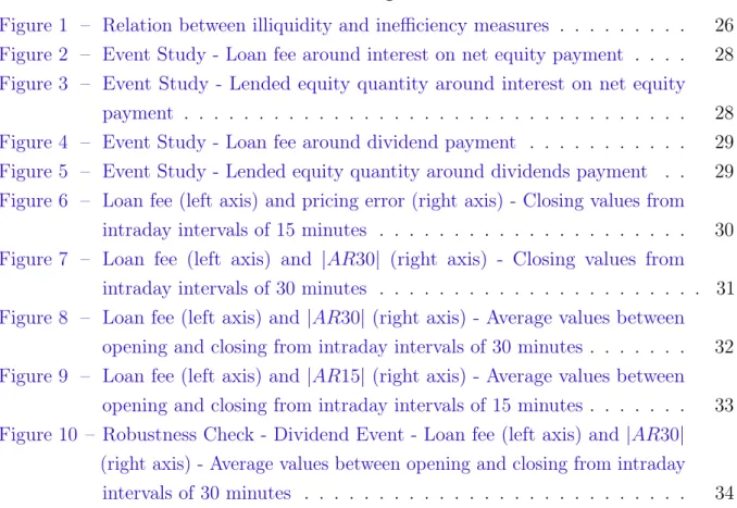
To address a possible doubt about the difference between inefficiency and illiquidity, figure 1 shows that the correlation between those concepts is not perfect. Using data from 2001 to 2013 it is possible to check that about 12% of stocks can be classified as efficient and illiquid, another 11% are unefficient, yet liquid. A close look in each group of stocks shows that blue ships, such as Petrobrás, Vale do Rio Doce, Eletrobrás and bank companies are liquid and efficient. Small firms, by the other hand, tend to be illiquid and unefficient.
It could be argued8
that the analysis carried out on table4suffers from endogeneity problems once is not possible to guarantee that unobserved shocks are not driving simultaneously loan fees and efficiency. The event study reported in next section and based on a tax arbitrage opportunity is the way how this issue will be overcome.
5.2
High frequency indexes exercises
5.2.1
Event study of tax arbitrage
During the period contained in the database, it was common in the market a type of operation called as "barriga de aluguel" by Brazilian traders. This is a tax arbitrage operation in which investment funds borrow stocks from individual entities for time enough to receive interest on net equity payments made by the firm company whose stock has
8
been lent9
. These earnings are received by funds without income tax discount10
, but when they return the stocks to the lender, the interest on net equity is subject to Brazilian 15% capital gains tax. This amount is appropriated by funds themselves and not paid to the government.
It was verified that this type of operation disturbed temporarily the equity lending market around days of interest on net equity payment. Both the average loan fee and the amount of equity stocks lent increased significantly on the period.
The methodology used in figures 2and3is described as follows: with the database of gain earnings (dividend and interest on net equity), an event study was carried out on dates when interest on net equity is paid. Day 0 refers to IoNE date, which is the last day that a stock could be bought on spot market with the right to receive interest on net equity. Due settlement in D+3 in this market, the definition of who receives the profit value will be based on stocks held in custody on day 3 (3 days after IoNE date).
There is a mismatch of deadlines between equity lending and spot market. Since equity lending settlement takes place on D+0, even if a fund borrow a stock on 3, it will be to legal matters the one entitled to receive the value of interest on net equity paid. At the end of the contract period, it must return to the lender the stock, interest on net equity and equity lending fee settled. Lending an equity on 3, receiving a tax-free gain and returning it at 4 tax-deducted is excellent to funds that appropriate the 15% taxation without being exposed to stock price risk11
.
The only way of sharing such tax gain with the lender is through loan fee, which increases significantly at the period. Figure 2shows the average loan fee done with stocks around dates where interest on net equity was paid. Figure 3 shows the ratio of the average amount of shares lent over the amount of stocks available to be traded. Besides the increase in loan fee, there is an increase on equity lending amount, which shows that individual investors also become more active as lenders who take advantage of this arbitrage opportunity. However, risk analysis is slightly distinct for these investors: the price risk of a stock is still existent, even when the stock is lent. In addition, this option of selling the stocks in spot market is put aside while they are being lent.
This kind of operation, however, ended at the beginning of 2015 due to law 13.043 enacted in November 201412
which established that interest on net equity was subject to
9
Equity lending borrowers also acquire the right to receive eventual earnings paid in the period that they still have the stocks in their portfolio.
10
During this period, funds were not taxed over profits from interest on net equity payment.
11
It happens because the fund does not sell the stocks it borrows, what is done in a regular short selling deal. It returns the exact same papers that it has borrowed, without being expoused to its price variation.
12
15% of income tax even for investment funds. Despite the similarity between IoNE and dividends as a way of companies pass on their earning to shareholders, equity lend market do not react in the same way in both cases. Figures ??and ?? show that, at least from 2009 to 2011, there was no significant change in loan fees or equity lent around days of dividend payment. This fact strengthens that tax arbitrage is the main force changing equity lend market.
Other studies have shown this market change. Saffi and Sigurdsson [2011], for example, recognized the anomaly on their database of equity lending and opt to remove all deals that are at least three weeks away from dividend payment on counties in which this kind of fiscal arbitrage is possible. This way, their results do not suffer influence from this uniqueness.
In Brazil, this opportunity of arbitrage increases equity lending deals in about five times and raises the equity lending fee by almost 100%. Through, it is clear that the entire market turn its attention to fiscal arbitrage in this period, leaving the investor that really wants to short sell extremely constrained.
As exposed, in this period there is a short selling constraint that is not related to (i) any fundamental situation of the firm (it is only necessary to pay interest on net equity); (ii) the spot market price of underlying asset or (iii) any macroeconomic indicator. It is an ideal exogenous event for the study of the constraint impact of short selling on price efficiency.
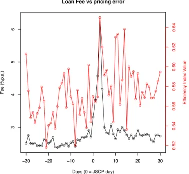
Results point to a positive relation between short selling constraint and price inefficiency in the period. It is not only equity loan fee and the amount of equity lent that shifts around the period of interest on net equity payment; inefficiency also rises significantly, as shown on figures 6 and 7.
Those images show the relation between short selling constraint and market efficiency. In figure 6 pricing error was used as a measure of high frequency inefficiency index. Figure 7 uses |��30| index, calculated with the closing values of intervals.
Critiques can be made when working with high frequency data from markets that are not so liquid. The "bid-ask bounce"13
induces a negative correlation between returns in high frequency analysis. To mitigate this point, the returns are calculated using the average value between opening and closing price of the interval. The results can be
13
evaluated on images 8 (for the 30 minute interval) and 9 (for the 15 minute interval). Volatility of efficiency index is reduced, which indicates that "bid-ask bounce" is a problem to be taken into consideration in this analysis. On these images, the increase of inefficiency at the period is even more evident. On figure 10 it is possible to check that around dividend payment the average efficiency is not affected.
Beyond graphic analysis, a mean test was made around interest on net equity payment date for each of graphics shown. The results are reported in table 5. Constant value represents the price efficiency index mean on days that are not explicitly tabulated. Coefficient values are the difference between the efficiency index for that specific day and the constant.
Using Beveridge Nelson pricing error index (column 1), the evidence of an inef-ficiency raise in D+3 is significant at 10% level. For |��30| index with closing values (column 2), D+3 coefficient is positive and significant at 5% level. In line with the discussion made, to reduce autocorrelation generated by construction on high frequency data (“bid-ask bounce”), when using the mean value between opening and closing prices of data interval to calculate |��30| (column 3) the coefficient is positive and significant at 1% level. The same happens with |��15| (column 4). Column 5 shows the values for dividend period: as expected there is no difference between the days after dividend pay days and the period average.
6 Conclusion
As exposed, the relation between efficiency and other stock characteristics was studied, as well as its behavior over time. Evidences were found that stocks that are more efficient are more liquid, more value, mostly traded, and belong to bigger companies and with a higher traded volume than stocks with less efficient price.
Evidences also shown the possibility of paying a risk premium to investors that maintain less efficient stocks in their portfolio. This premium exists even if controlled by the main risk factors documented in literature: market premium, SMB, HML, momentum and liquidity.
Besides efficiency analysis carried out, there are evidences of positive relation between price efficiency and short selling. On average, constrained portfolios have more inefficient prices: a raise of 1 standard deviation on the loan fees leads to an increase of approximately 0.04 standard deviations on low frequency efficiency indexes1
.
Considering days around payment of interest on net equity that created until 2014 an opportunity of fiscal arbitrage and constrained exogenously the market of short selling, it was found that short selling constraint is associated to an increase in price inefficiency. This analysis has been made using high frequency data.
If efficiency is a risk premium statistically significant and there is an efficiency reduction during the period of IoNE payment, abnormal returns reported by [Bonomo et al.,2015] could be interpreted as a premium demanded by market agents to hold less efficient stocks in their portfolio.
In summary, short selling constraints have a negative effect on market efficiency, consequently, constraining such deals makes prices further from their fundamentals.
1
References
Viral V. Acharya and Lasse H. Pedersen. Asset pricing with liquidity risk. CEPR Discussion Paper, No. 4718, 2004. URL http://ssrn.com/abstract=646661.
Michael J. Aitken, Alex Frino, Michael S. McCorry, and Peter L. Swan. Short sales are almost instantaneously bad news: Evidence from the australian stock exchange.
The Journal of Finance, 53(6):2205–2223, 1998. URLhttp://dx.doi.org/10.1111/ 0022-1082.00088.
Yang Bai, Eric C. Chang, and Jiang Wang. Asset prices under short-sale constraints, 2006.
Stephen Beveridge and Charles R. Nelson. A new approach to decomposition of eco-nomic time series into permanent and transitory components with particular atten-tion to measurement of the ‘business cycle’. Journal of Monetary Economics, 7(2): 151–174, 1981. URLhttp://www.uh.edu/~cmurray/courses/econ_7395/Beveridge% 20Nelson.pdf.
BM&FBOVESPA. Estatísticas btc. 2015. URL http://www.bmfbovespa.com.br/ BancoTitulosBTC/Estatisticas.aspx?Idioma=pt-br.
Ekkehart Boehmer and E. Kelley. Institutional investors and the informational efficiency of prices. Review of Financial Studies, 22:3563–3594, 2009. URL http://ssrn.com/ abstract=972620.
Ekkehart Boehmer and Juan (Julie) Wu. Short selling ansd the price discovery process.
Review of Financial Studies, 26:287–322, 2012. URL http://ssrn.com/abstract= 972620.
Marco Bonomo, João M. P. De Mello, and Lira Mota. Short-selling restrictions and returns: a natural experiment. 2015. URLhttps://ideas.repec.org/p/red/sed015/ 1353.html.
Brasil. Lei n 13.043, de 13 de novembro de 2014. 2014. URL http://www.planalto.gov. br/ccivil_03/_ato2011-2014/2014/Lei/L13043.htm.
Fernando Chague, Rodrigo De-Losso, Alan De Genaro, and Bruno Giovannetti. Short-selling and inside information. Departamento de Economia FEA-USP. Working Paper Series, 06, 2013. URL http://ssrn.com/abstract=2297342.
Fernando Chague, Rodrigo De-Losso, Alan De Genaro, and Bruno Giovannetti. Short-sellers: Informed, but restricted. Journal of International Money and Finance, 2014a. URL http://ssrn.com/abstract=2291235.
Fernando Chague, Rodrigo De-Losso, Alan De Genaro, and Bruno Giovannetti. Testing the effects of short-selling restrictions on asset prices. Departamento de Economia FEA-USP. Working Paper Series, 2014b. URL http://papers.ssrn.com/sol3/papers.
cfm?abstract_id=2135285.
John H. Cochrane. Time Series for Macroeconomics and Finance. University of Chicago, 1997. URL http://faculty.chicagobooth.edu/john.cochrane/research/papers/ time_series_book.pdf.
D. Diamond and R. Verrecchia. Constraints on short-selling and asset price adjustment to private information. Journal of Financial Economics, 18(3):277–311, 1987. URL http://dx.doi.org/10.1016/0304-405X(87)90042-0.
Eugene F. Fama. Efficient capital markets: A review of theory and empirical work.
The Journal of Finance, 25(2):383–417, 1970. URL http://dx.doi.org/10.1111/j. 1540-6261.1970.tb00518.x.
I. Goldstein and A. Guembel. Manipulation and the allocational role of prices. Review of Economic Studies, 75:133–164, 2008. URL http://finance.wharton.upenn.edu/ ~itayg/Files/manipulation-published.pdf.
Gustavo Grullon, Sébastien Michenaud, and James P. Weston. The real effects of short-selling constraints. Review of Financial Studies, 2015. URL http://rfs. oxfordjournals.org/content/early/2015/02/12/rfs.hhv013.abstract.
Campbell R. Harvey, Yan Liu, and Heqing Zhu. ... and the cross-section of expected returns. pages 159–178, 2014. URL http://ssrn.com/abstract=2249314.
Joel Hasbrouck. Assessing the quality of a security market: a new ap-proach to transaction cost measurement. The Review of Financial Studies, 6 (1):191–212, 1993. URL http://www.uic.edu/classes/actg/actg593/Readings/
K Hou and T. Moskowitz. Market frictions, price delay, and the cross-section of expected returns. Review of Economic Studies, 18:981–1020, 2005. URL http: //rfs.oxfordjournals.org/content/18/3/981.full.pdf.
Massimo Massa, Bohui Zhang, and Hong Zhang. The invisible hand of short sell-ing: Does short selling discipline earnings management? Review of Financial Stud-ies, 2014. URLhttp://rfs.oxfordjournals.org/content/early/2014/12/23/rfs. hhu147.abstract.
Table 1 – Correlation between low frequency efficiency metrics
Correlation �cross �1 D1 D2
�cross 1
�1
0.3922 1
D1 0.4990 0.1985 1
D2 0.4675 0.1103 0.8582 1
The table reports the correlation between low frequency efficiency index. �cross is the correlation between stock returns and lagged returns of NEFIN Market Factor. �1
24 2001 2002 2003 2004 2005 2006 2007 2008 2009 2010 2011 2012 2013 2014 mean
Illiquidity Index P1 0.0083 0.0133 0.0054 0.0044 0.0107 0.0076 0.0084 0.0193 0.0371 0.0097 0.0143 0.0133 0.0081 — 0.0123 P2 0.0098 0.0151 0.0059 0.0062 0.0137 0.0084 0.0108 0.0684 0.0239 0.0159 0.1273 0.0139 0.0172 — 0.0259 P3 0.0099 0.0091 0.0048 0.0100 0.0079 0.0131 0.0162 0.1349 0.0728 0.0209 0.0376 0.0253 0.0236 — 0.0297 P4 0.0349 0.0218 0.0078 0.0083 0.0318 0.0176 0.0515 0.2321 0.0837 0.0233 0.0355 0.0764 0.0302 — 0.0504
BM P1 1.13 1.27 1.50 0.76 0.59 0.43 0.65 0.64 0.72 0.64 0.68 0.87 0.84 0.98 0.84 P2 0.70 1.57 0.84 0.90 0.52 0.77 0.40 0.56 0.62 0.61 0.71 0.82 1.15 1.05 0.80 P3 1.20 0.68 0.85 0.56 0.92 0.42 0.40 0.59 0.70 0.54 0.55 0.55 0.81 1.00 0.70 P4 1.24 0.86 0.65 0.45 0.51 0.37 0.25 0.49 0.45 0.45 0.49 0.42 0.48 0.50 0.54
Num. Deals P1 222 277 399 582 587 799 1635 2738 2718 4368 7365 7066 9686 8709 3,368 P2 294 169 244 369 438 835 883 1373 1619 2533 2303 5701 5816 5447 2,002 P3 175 262 217 345 530 479 789 777 2035 1871 2241 3178 3655 5440 1,571 P4 93 149 213 289 265 368 277 573 1304 1125 1412 2317 2568 2352 950
Market Value (R$ M) P1 6253 3931 5687 14409 9317 23677 24968 27554 20089 34192 31998 17761 29945 20749 19,323 P2 5183 2979 3198 7951 12589 13958 18079 10300 8701 11080 12967 21160 12015 10281 10,746 P3 2746 5277 4550 4242 13499 5099 12140 7564 12831 7266 6821 9482 7929 13856 8,093 P4 1928 4301 6667 3873 4302 7501 3100 3702 3964 5543 4752 7814 4971 3025 4,674
Volume (R$ M) P1 8036 11384 16512 32212 22543 39123 88589 94969 52636 100761 109454 60524 101893 83078 58,694 P2 14197 4381 8460 12222 19617 39240 32325 31326 30270 35545 24025 70628 45421 35810 28,819 P3 5779 8211 6681 10632 28472 15149 29330 16315 41561 25049 20024 29968 25542 39573 21,592 P4 1823 5770 8759 7543 8499 13757 11007 13496 20383 12789 15763 20992 19511 10628 12,194
Table 3 – Efficiency sorted portfolios - Regression results
VARIABLES P1 P2 P3 P4 P4 - P1
�me 0.996*** 0.926*** 0.879*** 0.872*** -0.124***
(0.00732) (0.00757) (0.00809) (0.00882) (0.0106)
SMB 0.188*** 0.175*** 0.220*** 0.369*** 0.181***
(0.0152) (0.0158) (0.0168) (0.0184) (0.0222)
HML 0.154*** 0.0581*** 0.0147 -0.0607*** -0.215***
(0.0114) (0.0118) (0.0126) (0.0137) (0.0166)
WML -0.164*** -0.0987*** -0.0405*** 0.00458 0.169***
(0.00976) (0.0101) (0.0108) (0.0118) (0.0142)
IML -0.0966*** -0.0307* 0.0688*** 0.0652*** 0.162***
(0.0154) (0.0159) (0.0170) (0.0185) (0.0224)
Constant 0.000100 0.000160 0.000221** 0.000239** 0.000138 (0.000101) (0.000104) (0.000111) (0.000121) (0.000146)
Observations 3,281 3,281 3,281 3,281 3,281
R-squared 0.894 0.864 0.822 0.788 0.256
Standard errors in parentheses *** p<0.01, ** p<0.05, * p<0.1
The table reports the regression results of P1 to P4 and P1-P4 on the main risk factors of financial literature. P1 to P4 are portfolios with efficiency sorted stocks, equally weighed. P1 is composed of stocks of the most efficient quartile and P4 stocks from the less efficient quartile, yearly balanced. P4 - P1 is a zero cost portfolio that buys P4 and sells P1. The return series of each of these 5 portfolios is the dependent variable in each respective column. As explaining variables are used: �e
m, NEFIN market factor discounted the Brazilian risk
Figure 1 – Relation between illiquidity and inefficiency measures
0.00 0.05 0.10 0.15 0.20 0.25
0.00
0.05
0.10
0.15
0.20
0.25
Illiquidity Index
In
e
ff
ici
e
n
cy
In
d
e
x
Table 4 – Impacts of short selling constraints on price efficiency - Low Frequency Analysis
1 2 3 4 5 6
VARIABLES D1 D1 D1 D2 D2 D2
Loan Fee 0.0425*** 0.0402*** 0.0358* 0.0379*** 0.0367*** 0.0433*
(0.0135) (0.0138) (0.0205) (0.0136) (0.0138) (0.0200)
dJSCP 0.0528 0.0577 0.0351 0.0586 0.0633 0.0537
(0.0390) (0.0392) (0.0519) (0.0391) (0.0394) (0.0510)
Size 0.00134 0.0529* -0.00243 0.0290
(0.0189) (0.0320) (0.0187) (0.0321)
Ret0 0.0449*** 0.0552*** 0.0514*** 0.0499**
(0.0145) (0.0211) (0.0143) (0.0212)
Illiq 0.1460*** 0.1141***
(0.0304) (0.0312)
Free Float -0.0162 0.0017
(0.0209) (0.0206)
Book-to-Market 0.0122 0.0164
0.0278 (0.0278)
Turnover -0.0240 -0.0177
(0.0236) (0.0225)
Constant -0.0442 -0.0480 0.1199* -0.137 -0.148 0.2571***
(0.0786) (0.0871) (0.0659) (0.0840) (0.0924) (0.0625)
Observations 4,803 4,640 4,612 4,803 4,640
R-squared 0.128 0.130 0.146 0.111 0.113
Robust standard errors in parentheses *** p<0.01, ** p<0.05, * p<0.1
The table reports the regression results of D1 and D2 on Loan Fee and others controls for a panel data of stocks from 2009 to July 2011. D1 (R2 ratio) and D2 (Betas ratio),
dependent variables, are efficiency index described on section 4. As explicative, it’s used
Figure 2 – Event Study - Loan fee around interest on net equity payment
X-axis is days around interest on net equity payment (day 0), Y-axis is the average loan fee charged on equity lending deals at %p.a. The "JSCP day" (IoNE date) is the last day to have the stock and qualify to receive the interest on net equity. Due settlement in D+3 in the spot market, the definition of who receives the gain value will be based on stocks held in custody on day 3 (3 days after in-INE). Data used is from 2009 to July 2011.
Figure 3 – Event Study - Lended equity quantity around interest on net equity payment
Figure 4 – Event Study - Loan fee around dividend payment
-30 -20 -10 0 10 20 30
1.5
2.0
2.5
3.0
3.5
Days (0 = Div. day)
L o a n f e e (% a .y. )
X-axis is days around dividend payment (day 0), Y-axis is the average loan fee charged on equity lending deals at %p.a. The "Div. day" is the last day to have the stock and qualify to
receive dividends. Data used is from 2009 to July 2011.
Figure 5 – Event Study - Lended equity quantity around dividends payment
-30 -20 -10 0 10 20 30
0.5
1.0
1.5
2.0
2.5
Days (0 = Div. day)
Sh a re s L e n t / Sh a re s O u tst a n d in g (p e r 1 0 0 0 )
Figure 6 – Loan fee (left axis) and pricing error (right axis) - Closing values from intraday intervals of 15 minutes
● ● ●●● ●●● ●● ●● ● ●●●●● ● ● ●● ● ●●●●● ● ● ● ● ● ● ● ● ●● ● ● ● ● ● ● ● ● ● ● ● ● ● ●●●●● ●● ●●●
−30 −20 −10 0 10 20 30
3
4
5
6
Days (0 = JSCP day)
F ee (%p .a.) ● ● ● ● ● ● ● ● ● ● ●● ● ● ● ● ● ● ● ● ● ● ● ● ● ● ● ● ● ● ● ● ● ● ● ● ● ● ● ● ● ● ● ● ● ● ● ● ● ● ● ● ● ● ● ● ●● ● ● ●
−30 −20 −10 0 10 20 30
Loan Fee vs pricing error
0.52 0.54 0.56 0.58 0.60 0.62 0.64 Efficiency Inde x V alue
Figure 7 – Loan fee (left axis) and|��30| (right axis) - Closing values from intraday intervals of 30 minutes
● ● ●●● ●●● ●● ●● ● ●●●●● ● ● ●● ● ●●●●● ● ● ● ● ● ● ● ● ●● ● ● ● ● ● ● ● ● ● ● ● ● ● ●●●●● ●● ●●●
−30 −20 −10 0 10 20 30
3
4
5
6
Days (0 = JSCP day)
F ee (%p .a.) ● ● ● ● ● ● ● ● ● ● ● ● ● ● ● ● ● ● ● ● ●● ● ● ● ● ● ● ● ●● ● ● ● ● ● ● ● ● ● ● ● ● ● ● ● ● ● ● ● ● ● ● ●●● ● ● ● ● ●
−30 −20 −10 0 10 20 30
Loan Fee vs |AR 30|
0.16 0.17 0.18 0.19 0.20 0.21 0.22 Efficiency Inde x V alue
Figure 8 – Loan fee (left axis) and |��30|(right axis) - Average values between opening and closing from intraday intervals of 30 minutes
● ● ●●● ●●● ●● ●● ● ●●●●● ● ● ●● ● ●●●●● ● ● ● ● ● ● ● ● ●● ● ● ● ● ● ● ● ● ● ● ● ● ● ●●●●● ●● ●●●
−30 −20 −10 0 10 20 30
3
4
5
6
Days (0 = JSCP day)
F ee (%p .a.) ● ● ● ● ● ● ● ● ● ● ● ● ● ● ● ● ● ● ● ● ● ● ● ●● ● ● ● ● ● ●● ● ● ● ● ● ● ● ● ● ● ● ● ● ● ● ● ● ● ● ● ● ● ● ● ● ● ● ● ●
−30 −20 −10 0 10 20 30
Loan Fee vs |AR 30|
0.16 0.17 0.18 0.19 0.20 0.21 Efficiency Inde x V alue
Figure 9 – Loan fee (left axis) and |��15|(right axis) - Average values between opening and closing from intraday intervals of 15 minutes
● ● ●●● ●●● ●● ●● ● ●●●●● ● ● ●● ● ●●●●● ● ● ● ● ● ● ● ● ●● ● ● ● ● ● ● ● ● ● ● ● ● ● ●●●●● ●● ●●●
−30 −20 −10 0 10 20 30
3
4
5
6
Days (0 = JSCP day)
F ee (%p .a.) ● ● ●● ● ● ● ● ● ● ● ● ● ● ● ● ● ● ● ● ● ● ● ● ● ● ● ● ● ● ● ● ● ● ● ● ● ● ● ● ● ● ● ● ● ● ● ● ● ● ● ● ● ● ● ● ● ● ● ● ●
−30 −20 −10 0 10 20 30
Loan Fee vs |AR 15|
0.15 0.16 0.17 0.18 0.19 0.20 0.21 Efficiency Inde x V alue
Figure 10 – Robustness Check - Dividend Event - Loan fee (left axis) and |��30| (right axis) - Average values between opening and closing from intraday intervals of
30 minutes
X-axis is days around dividend payment (day 0), Y-axis (left) is average loan fee charged on equity lending deals at %p.a., Y-axis (right) is average first order autocorrelation. Average values between opening and closing from intraday intervals of 30 minutes were used on calculation. It was done to prevent "bid-ask bounce". The lower the index is, more efficient stock
Table 5 – Mean test around interest on net equity payment date - High Frequency Analysis
1 2 3 4 5 (div)
VARIABLES BN |��30| |��30| |��15| |��30|
close value close value open-close mean open-close mean open-close mean
D-4 -0.0415 -0.00225 0.00564 0.0016 0.0001 (0.0387) (0.0158) (0.0151) (0.0142) (0.0102) D-3 -0.041 -0.00697 -0.00823 0.000485 -0.0078
(0.0389) (0.0156) (0.015) (0.0141) (0.0101) D-2 0.0227 0.0117 0.016 0.013 -0.0201**
(0.0389) (0.0155) (0.0149) (0.0141) (0.0098) D-1 -0.034 0.00324 0.00503 -0.00946 -0.0175* (0.0386) (0.0155) (0.0149) (0.014) (0.0102) D+0 -0.00764 0.00401 0.0105 0.014 -0.0014
(0.0389) (0.0152) (0.0146) (0.0139) (0.0096) D+1 -0.015 -0.00613 0.0102 -0.00526 -0.0128
(0.0385) (0.0155) (0.0149) (0.0139) (0.0096) D+2 -0.00199 0.00178 0.004 -0.000338 -0.0001
(0.0377) (0.0154) (0.0147) (0.0136) (0.0094) D+3 0.0722* 0.0383** 0.0390*** 0.0375*** 0.0152
(0.0379) (0.0157) (0.0151) (0.0139) (0.0102) D+4 0.0408 0.0228 0.0186 0.0261* -0.0046
(0.0382) (0.0155) (0.0149) (0.0137) (0.0099) D+5 0.0127 0.00944 -0.00198 0.00276 -0.0117
(0.0393) (0.0156) (0.015) (0.0141) (0.0097) D+6 0.0201 -0.00222 -0.00368 0.0118 0.0048
(0.0383) (0.0156) (0.015) (0.0139) (0.0101) D+7 -0.00596 -0.025 -0.015 -0.000665 0.0193* (0.0384) (0.0158) (0.0151) (0.014) (0.0105) D+8 -0.0352 0.0124 0.0292* -0.00193 -0.0001
(0.039) (0.0157) (0.0155) (0.014) (0.0098) Constant 0.579*** 0.180*** 0.172*** 0.171*** 0.2450***
(0.00551) (0.00223) (0.00214) (0.00200) (.0014)
Observations 19,889 22,075 22,075 22,075 18,606 R-squared 0.000 0.001 0.001 0.001 0.001
Standard errors in parentheses *** p<0.01, ** p<0.05, * p<0.1