Quantitative genetics theory for non-inbred populations in linkage
disequilibrium
José Marcelo Soriano Viana
Universidade Federal de Viçosa, Departamento de Biologia Geral, Viçosa, MG, Brazil.
Abstract
Although linkage disequilibrium, epistasis and inbreeding are common phenomena in genetic systems that control quantitative traits, theory development and analysis are very complex, especially when they are considered together. The objective of this study is to offer additional quantitative genetics theory to define and analyze, in relation to non-inbred cross-pollinating populations, components of genotypic variance, heritabilities and predicted gains, assuming linkage disequilibrium and absence of epistasis. The genotypic variance and its components, additive and due to dominance genetic variances, are invariant over the generations only in regard to completely linked genes and to those in equilibrium. When the population is structured in half-sib families, the additive variance in the parents’ generation and the genotypic variance in the population can be estimated. When the population is structured in full-sib families, none of the components of genotypic variance can be estimated. The narrow sense heritability at plant level can be estimated from the parent-offspring or mid parent-offspring regression. When there is dominance,
the narrow sense heritability estimate in the in F2is biased due to linkage disequilibrium when estimated by the
Warner method, but not when estimated by means of the plant F2-family F3regression. The bias is proportional to the
number of pairs of linked genes, without independent assortment, and to the degree of dominance, and tends to be positive when genes in the coupling phase predominate or negative and of higher value when genes in the repulsion phase predominate. Linkage disequilibrium is also cause of bias in estimates of the narrow sense heritabilities at full-sib family mean and at plant within half-sib and full-sib families levels. Generally, the magnitude of the bias is proportional to the number of pairs of genes in disequilibrium and to the frequency of recombining gametes. Key words:components of genotypic variance, heritabilities, half-sib families, full-sib families.
Received: August 26, 2003; Accepted: June 25, 2004.
Introduction
Linkage disequilibrium, epistasis and inbreeding are phenomena that when considered separately or especially together, make the characterization and analysis of genetic systems responsible for quantitative traits very complex. Although the fundamental theory for each was established many years ago (Cockerham, 1954, 1956; Kempthorne, 1955, 1957; Schnell, 1961, 1963; Cockerham and Weir, 1977), discussion on linkage disequilibrium and epistasis related to breeding is surprisingly uncommon in statistical genetics (Kempthorne, 1973), quantitative genetics (Wricke and Weber, 1986; Hallauer and Miranda Filho, 1988; Comstock, 1996; Falconer and Mackay, 1996; Lynch and Walsh, 1998) and biometrical genetics (Mather and Jinks, 1974; Kearsey and Pooni, 1996) books, compared to other subjects relevant to breeders. Linkage disequilibrium and absence of epistasis are compulsorily assumed in al-most all the methodologies developed to analyze
quantita-tive traits. The consequence, clearly, is biased estimates of genetic parameters and predicted gains, as linkage and genic interaction are the rule and not the exception.
Although relevant, knowledge of the effects of link-age disequilibrium on the coefficients of the components of genotypic variance, including epistasis, on the covariance between relatives (Cockerham, 1956; Schnell, 1961, 1963; Weiret al., 1980) does not represent all the theory of
quan-titative genetics for polygenic systems with genes in dis-equilibrium. The objective of this study was to supply additional theoretical information, characterizing and ana-lyzing the components of genotypic variance, the heritabilities and the expected gains from selection, in rela-tion to non-inbred cross-pollinating popularela-tions, assuming absence of epistasis.
Theory and Discussion
Components of genotypic variance
In the gametic pool of a non-inbred population (gen-eration n), the probabilities of the gametes AB, Ab, aB and ab are (Kempthorne, 1973)
Copyright by the Brazilian Society of Genetics. Printed in Brazil www.sbg.org.br
Send correspondence to José Marcelo Soriano Viana. Universi-dade Federal de Viçosa, Departamento de Biologia Geral, 36.570-000 Viçosa, MG, Brazil. E-mail: [email protected].
p p p
p p q
p q p
p 11 (n) a b (n) 10 (n) a b (n) 01 (n) a b (n) 0 = + = − = − ∆ ∆ ∆ 0 (n) a b (n) q q = + ∆
where p is the probability of the gene that increases the trait expression, q is the probability of the allelic gene that de-creases it and∆(n)
11 (n) 00 (n) 10 (n) 01 (n)
= p p −p p is the measure of
link-age disequilibrium. The genotype probabilities in generation 0 are
[ ]
f p p 2p p
f p p q 2p
22 (0) a 2 b 2 a b 21 (0) a 2
b b a
= + +
= +
− −
∆( )1 ∆( )1 2
2
[ ]
[ ]
(q - p
f p q 2p q
b b 20 (0) a 2 b 2 a b ) ( ) ( ) ( ) ( ) ∆ ∆ ∆ ∆ − − − − − = − +
1 1 2
1 1
2
2
[ ]
f p q p 2(q - p p
f p
12 (0)
a a b 2
a a b
11c (0) a = + − = − − 2 2 2
1 1 2
) ∆( ) ∆( )
[ ]
q p q 2p p 2q q
f p q p
a b b a b a b
11r (0) a a + + + = − − −
∆( )1 ∆( )1 ∆( )1 2 2
2 b b a b a b
[ ]
10 (0)
a a b 2
q 2p q 2q p
f p q q 2
− − +
= −
− − −
∆( )1 ∆( )1 2 ∆( )1 2
2 (q - p qa a) b
[ ]
( ) ( )
∆−1 − ∆−1 2 2
[ ]
f q p 2q p
f q p q 2q
02 (0) a 2 b 2 a b 01 (0) a 2
b b a
= − +
= −
− −
∆( )1 ∆( )1 2
2
[ ]
[ ]
(q - p
f q q 2q q
b b 00 (0) a 2 b 2 a b ) ( ) ( ) ( ) ( ) ∆ ∆ ∆ ∆ − − − − − = + +
1 1 2
1 1
2
2
where fijis the probability of carrier of i and j copies of the
genes of loci A and B that increase the trait expression, re-spectively. The c and r indexes identify the double-heterozygotes in the coupling and repulsion phases.
The genotypic values are
G (m a ) (m a ) (M A D ) (M A D ) G (
22 a a b b a AA AA b BB BB 12
= + + + = + + + + +
= m d ) (m a ) (M A D ) (M A D ) G (m a
a a b b a Aa Aa b BB BB 02 a a
+ + + = + + + + +
= − ) (m+ b+a ) (Mb = a+Aaa+D ) (Maa + b+ABB+D )BB
G (m a ) (m d ) (M A D ) (M A D ) G (
21 a a b b a AA AA b Bb Bb 11
= + + + = + + + + +
= m d ) (m d ) (M A D ) (M A D ) G (m a
a a b b a Aa Aa b Bb Bb 01 a a
+ + + = + + + + +
= − ) (m+ b+d ) (Mb = a+Aaa+D ) (Maa + b+ABb+D )Bb
G (m a ) (m a ) (M A D ) (M A D ) G (
20 a a b b a AA AA b bb bb 10
= + + − = + + + + +
= m d ) (m a ) (M A D ) (M A D ) G (m a
a a b b a Aa Aa b bb bb 00 a a
+ + − = + + + + +
= − ) (m+ b−a ) (Mb = a+Aaa+D ) (Maa + b+Abb+D )bb
where, for each gene, m is the mean of the genotypic values of the homozygotes, a is the deviation between the genotypic value of the homozygote of greatest expression and m, d is the deviation due to dominance, M = m + (p - q)a + 2pqd is the population mean, A is additive genetic value and D is genetic value due to dominance. Regarding one
gene, A = 2qαand D = -2q2d, if the individual is
homozy-gous for the gene that increases the trait expression, or A =
(q - p)αand D = 2pqd, if the individual is heterozygous, or
A = -2pαand D = -2p2d, if the individual is homozygous for
the gene that reduces the trait expression, whereα= a + (q
-p)d is the average effect of a gene substitution (Falconer and Mackay, 1996).
The genotypic mean of generation 0 is
E(G) f (G ) f (G ) m (p q )a
2p q d 22
(0)
22 00
(0)
00 a a a a
a a
= + +K = + − +
a +mb +(pb −q )ab b +2p q db b b =M The genotypic variance is
σ α G 2(0) 22 (0) 22 2 00 (0) 00 2 2
a a a 2
f (G ) f (G ) M
(2p q 2p
= + + − =
+
K
b b b
2 (-1) a b a 2 a 2 a 2 b 2 b 2 b 2 (-1)
q + 4 ) +
(4p q d 4p q d
α ∆ α α ∆
+ +8[( )]2d d ) a b A 2(0) D 2(0) = + σ σ where:
Cov(A , A ) 2
Cov(A , D ) Cov(D , A )
a b
(0) ( 1) a b a b (0) a b (0 = = −
∆ α α
)
a b
(0) ( 1)
a b
Cov(D , D ) d d
= = −
0
4[ ]2
∆
Considering k genes,
σ α α α
σ
A i i i
2 ij (-1) i j 1 k
i 1 < k
i 1 k
D
p q j
2 0 2 0 2 4 ( ) ( ) = + = = =
∑
∑
∑
∆ = + = = =∑
∑
∑
4 p q di 8 d d
2 i 2 i 2 ij (-1) i j 1 k
i 1 < k
i 1 k
j
[∆ ]2
In spite of the probabilities of the genotypes altering
from generation to generation, because∆ij ∆
(n)
ij ij (n-1) r )
= −(1 =
(1−r )ij
n∆(0)(Kempthorne, 1973), where r
ijis the frequency
of recombining gametes, the population mean is constant. The genotypic variance changes as the population ap-proaches equilibrium. The genotypic variance is invariant
only for completely linked genes (rij= 0) and those in
equi-librium (∆ij (n)
=0).
If generation 0 is the F2derived from the cross of two
pure lines, pi= 0, 1/2 or 1, and
∆ij
(-1) rij ij
2 r 2 = − −
1 2 2
, for coupling genes, and
∆ij
(-1) rij ij
2 r 2 = − − 2 2 1
, for repulsion genes
Among and within family genotypic variances
When the generation 0 is structured in half-sib fami-lies, the genotypic means of the progenies are
[
]
[
]
G p p (M A A D D ) +
p q (M
AABB (1)
a b AA BB AA BB
a b = + + + + + − + ∆ ∆ ( ) ( ) 0 0
[
]
[
]
q p (M A A D D ) +
q q (M A A D
a b Aa BB Aa BB
a b Aa Bb
− + + + + + + + + ∆ ∆ ( ) ( ) 0 0 Aa Bb
AA BB AABB
D ) =
M A A M 1
2A
+
+1 + = +
2
1 2
G M A A M 1
2A
G M A
AABb (1)
AA Bb AABb
aabb (1) aa = + + = + = + + 1 2 1 2 1 2 K 1
2A M
1
2A
bb = + aabb
Therefore, the genotypic mean of a half-sib family is also equal to the mean of the population plus half the addi-tive genetic value of the common parent. The among and within genotypic variances are
σGaHSF 2(1) 22 (0) AABB (1) 2 00 (0) aabb (1) 2
f (G ) ... f (G )
= + + − = = + − M2 A GwHSF 2(1)
A D A
1 4 1
4
2 0
2 1 2 1 2 0
σ
σ σ σ σ
( )
( ) ( ) ( )
Or further,
σGaHSF σ α α
2(1) A ij ij ij (0) i j 1 k r
1- r j
= + = 1 4
2 1( ) ∆
∑
∑
= = + − i 1 < k GwHSF 2(1) A D ij ij r 1- r
σ 3σ σ
4
2 1( ) 2 1( )
∆ij (0)
i j 1
k
i 1 < k j α α = =
∑
∑
ThusσA
2 0( )
and, depending on the sample data,σG
2 1( )
are estimable.
The genotypic mean of a full-sib family is, generi-cally,
G G G’
2 u d u d
FSF = a a b b
+ + + (u
i= 0, 1 or -1/2)
where G and G’ are the genotypic values of the parents. Thus,
σGaFSF σ
2(1) G a 2 a b 2 b a
d V(u ) d V(u )
d Cov(G G’ , u
= + + +
+
1 2
2 0( )
a b b
a b a b
) + d Cov(G G’ , u ) + 2d d Cov(u , u )
+
But,
[ ]
E(u ) 0 (i 1,... , k)
E (u ) 3p q (i 1,... , k)
i i 2 i 2 i 2 = = = =
[ ]
Cov(G G’ , u )a 4p q da 4 d
2 a 2 a (-1) b
+ = − − ∆ 2
[ ]
Cov(G G’ , u )b 4p q db 4 d
2 b 2 b (-1) a
+ = − − ∆ 2
[ ]
Cov(u , u )a b
(-1)
=3 ∆ 2
Thus,
σ σ σ
σ σ σ
GaFSF 2(1) A D GwFSF 2(1) A D = + = + 1 2 1 4
2 0 2 0
2 1 2
( ) ( )
( ) (1 1 2 0 2 0
2
1 4
) ( ) ( )
− σA − σD
Or further,
σGaFSF σ σ
2(1) A D ij ij ij ( r 1- r = + + 1 2 1 4 2
2 1( ) 2 1( )
∆
[ ]
0) i j 1 ki 1 < k ij ij (0) j 1 1- r α α = =
∑
∑
+ − 2 1 2∆ 2d di j 1
k
i 1 < k
j
= =
∑
∑
σGwFSF σ σ
2(1) A D ij ij ij ( r 1- r = + − 1 2 3 4 2
2 1( ) 2 1( )
∆
[ ]
0) i j 1 ki 1 < k ij ij (0) j 1 1- r α α = =
∑
∑
− − 2 1 2∆ 2d di j 1
k
i 1 < k
j
= =
∑
∑
In this case, no component of the genotypic variance is estimable.
Heritabilities and genetic gains
The narrow sense heritability at individual level in the generation 0 is the square of the correlation between the phenotypic and additive genetic values (Falconer and MacKay, 1996; Viana, 2002), given by
h2 A
2(0)
P 2(0)
=σ σ
Its estimation, although rare, can be done by the re-gression of the mean phenotypic value of non-inbred prog-eny (generation 1) as a function of the phenotypic value of a parent or of the mean phenotypic value of the parents (gen-eration 0) (Hallauer and Miranda Filho, 1988). Assuming that the genotypic value and environmental effect are inde-pendent variables, the parent-offspring covariance is
Cov(P , O f (A D ) 1
2A
f
(0) (1) 22 (0)
22 22 22
00 ( )= + ... + + 0)
00 00 00 A
(A D ) 1
2A
+
−00=
1 2
2 0
. ( )
σ
The parent-grand offspring covariance is
Cov(P , O f (A D ) 1
4A
f
(0) (2) 22 (0)
22 22 22
00 ( )= + ... + + 0)
00 00 00 A
(A D ) 1
4A
+
−00=
1 4
2 0
. ( )
σ
Cov(P , O(0) (n)
n
A 2(0) )=
1
2 σ
The covariance between S0plant and S1progeny is
Cov(S , S Cov(G, G u d u d ) =
d Cov(G 0
(0) 1 (1)
a a b b
G 2(0)
a
)= + +
+
σ , u ) d Cov(G, u ) (ua + b b i=0 or −1 2/ )
But
[ ]
E(u ) p q (i 1,... , k)
E (u ) p q (i 1,... , k)
i i i
i 2
i i
= − =
=1 =
2
[
]
Cov(G, u ) p q q p p q d
q p
a a a a a a a a a
a a
(-1) b
= − − + −
− −
( )
( )
α
α
2
2
∆
[ ]
∆(-1) b d 2[
]
Cov(G, u ) p q q p p q d
q p
b b b b b b b b b
b b
(-1) a
= − − + −
− −
( )
( )
α
α
2
2
∆
[ ]
∆(-1) a d 2[ ]
Cov(u , u )a b qa pa qb pb
(-1) (-1)
= 1 − − +
2
2
( )( )∆ ∆
Thus, considering k genes,
[
]
Cov(S , S0 p q p -q d
(0) 1 (1)
A 2(0)
D 2(0)
i i i i i i
i
)= + + ( )
=
σ 1σ α
2
[
]
1 k
ij (-1)
i i i j j j j i
j 1 k
i 1 < k
p -q d p -q d
∑
∑
∑
+
+
= =
∆ ( ) α ( ) α
In the presence of dominance, the estimate of narrow sense heritability at F2plant level is biased because of
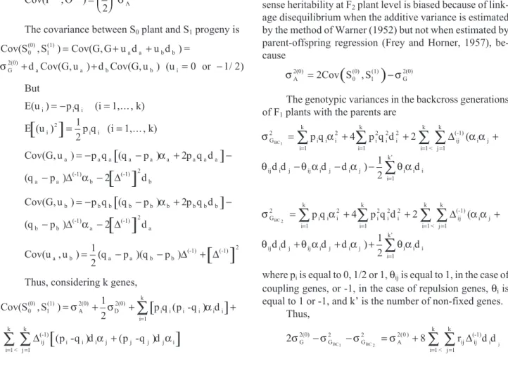
link-age disequilibrium when the additive variance is estimated by the method of Warner (1952) but not when estimated by parent-offspring regression (Frey and Horner, 1957), be-cause
(
)
σA σ
2(0)
0 (0)
1 (1)
G 2(0)
2Cov S S
= , −
The genotypic variances in the backcross generations of F1plants with the parents are
σ α2 2 α α
G 2
i i i i 1
k
i 2
i 2
i i 1
k
ij (-1)
i j
BC1 = p q + p q d + +
= =
∑
4∑
2 ∆ ( j 1k
i 1 < k
= =
∑
∑
θij i j θ αij i j iαj θ αi i i i 1 k’
d d − d −d − d
=
∑
) 1
2
σ α2 2 α α
G 2
i i i i 1
k
i 2
i 2
i i 1
k
ij (-1)
i j
BC 2 = p q + p q d + +
= =
∑
4∑
2 ∆ ( j 1k
i 1 < k
= =
∑
∑
θij i j θ αij i j iαj θ αi i i i 1 k’
d d + d +d + d
=
∑
) 1
2
where piis equal to 0, 1/2 or 1,θijis equal to 1, in the case of
coupling genes, or -1, in the case of repulsion genes,θiis
equal to 1 or -1, and k’ is the number of non-fixed genes. Thus,
2σG σ σ σ
2(0) G 2
G 2
A ij ij
(-1) i j 1
k
i
BC1 BC 2 r d dj
− − = +
=
∑
2 0( ) 8 ∆
=
∑
1 < k
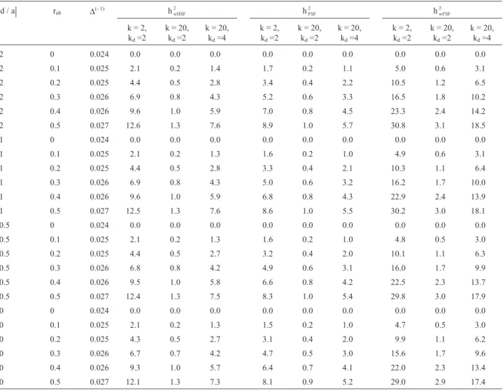
Table 1- Bias (%) in the estimate of the narrow sense heritability at F2plant level, obtained by the Warner method, considering k non-fixed genes (equal
allelic frequencies), kdgenes in disequilibrium, in coupling (c) and repulsion (r), and different degrees of dominance (d/a) and recombinant gamete
frequencies (rab).
d / a rab ∆( )−1, c k = 2,
kd=2, c
k = 20, kd=2, c
k = 20, kd=4, c
∆( )−1, r k = 2,
kd=2, r
k = 20, kd=2, r
k = 20, kd=4, r
The magnitudes of the bias in relation to polygenic systems with two and 20 genes, with groups of two and four in disequilibrium (Table 1), reveal that the heritability
esti-mates in F2, obtained by the Warner method and assuming
linkage equilibrium, can be very biased. Generally, the bias is proportional to the number of pairs of genes in disequilib-rium (linked without independent assortment) and to the degree of dominance, tending to be positive when genes in the coupling phase predominate and negative when genes in the repulsion phase predominate. In this case, the bias should have greater magnitude.
Therefore, linkage disequilibrium is not the cause of bias in predicting genetic gains from mass selection in cross-pollinating populations, with estimation of the addi-tive variance by the offspring or mid parent-offspring regression. In the presence of dominance, the pre-diction of gains with selection in F2is biased due to linkage
disequilibrium when the additive variance is estimated by the Warner method, but not when estimated by the par-ent-offspring regression.
The narrow sense heritability at half-sib family mean level is the square of the correlation between the mean phenotypic value of the progeny and the additive genetic value of the common parent (Viana, 2002), given by
h2 A
2(0)
PaHSF 2(1)
=( / )1 4σ σ
The narrow sense heritability at plant within family level, which corresponds to the square of the mean correla-tion, considering the different progenies, between the phenotypic and additive genetic values of the same individ-ual is
h
r 2
A 2(0)
ij ij (-1)
i j 1
k
i 1 < k
PwHSF 2(1
j =
−
= =
∑
∑
( / )3 4σ 4 α α
σ
∆
)
Linkage disequilibrium is, then, cause of bias only in predicting gain from within selection.
With full-sib families, the narrow sense heritabilities at progeny mean level, that is the square of the correlation between the progeny mean phenotypic value and the mean additive genetic value of the parents (Viana, 2002), and at plant within family level are
h2 A
2(0)
PaFSF 2(1)
=( / )1 2σ σ
h
r 1- r 2
A
2(1) ij
ij ij (0)
i j 1
k
i 1 j
=
−
= =
∑
( / )1 2σ 2 ∆ α α
< k
PwFSF 2(1)
∑
σ
Assuming linkage equilibrium, the estimated heritabilities are
h
r 2
A 2(0)
ij ij (-1)
i j 1
k
i 1 < k
PaFSF 2(1
j =
+
= =
∑
∑
( / )1 2σ 2 α α
σ
∆
[
]
[ ]
)
ij ij
(-1) i j 1
k
i 1 < k
PaFSF 2(1)
1- (1- r d d
j +
= =
∑
∑
4 )2
∆ 2
σ
h
r 1- r 2
A
2(1) ij
ij ij (0)
i j 1
k
i 1 j
=
+
= =
∑
( / )1 2σ 4 ∆ α α
[ ]
< k
PwFSF 2(1)
ij
ij (0)
i 1
1- r d d
∑
+
−
σ
2
4 1
2
∆ j
j 1 k
i 1 < k
PwFSF 2(1)
= =
∑
∑
σ
Therefore, the predicted gains with among and within selection are biased due to linkage disequilibrium.
The analysis of the bias due to linkage disequilibrium in the estimates of genetic population parameters is com-plex because of the infinite combinations of genotype and gene frequencies, degree of dominance, frequency of re-Table 1 (cont)
d / a rab ∆( )−1, c k = 2,
kd=2, c
k = 20, kd=2, c
k = 20, kd=4, c
∆( )−1, r k = 2,
kd=2, r
k = 20, kd=2, r
k = 20, kd=4, r
combining gametes, number of genes in the polygenic sys-tem and number of pairs of genes in disequilibrium. Considering two and 20 genes in the genic system, with groups of two and four in disequilibrium (Tables 2, 3 and 4), it can be seen that the bias in the narrow sense heritability estimates at plant within half-sib family level, at full-sib family level and at plant within full-sib progeny
level is generally reduced but may have a very high magni-tude, depending on the number of genes and the number of pairs of genes in disequilibrium. The bias is proportional to the number of genes, to the number of pairs of genes in dis-equilibrium and to the frequency of recombining gametes. The magnitude of the bias is minimized when the frequency of the dominant genes is intermediate. When the dominant
Table 2- Bias (%) in the estimates of the narrow sense heritabilities at plant within half-sib family (hwHSF2 ), at full-sib family mean (hFSF2 ) and at plant
within full-sib progeny levels (hwFSF2 ), considering k non-fixed genes, k
dgenes in disequilibrium, dominant genes at low frequencies (0.1 to 0.2), and
different degrees of dominance (d/a) and recombining gamete frequencies (rab).
d / a rab ∆(- 1) hwHSF
2 h
FSF
2 h
wFSF 2
k = 2, kd=2
k = 20, kd=2
k = 20, kd=4
k = 2, kd=2
k = 20, kd=2
k = 20, kd=4
k = 2, kd=2
k = 20, kd=2
k = 20, kd=4
2 0 0.024 0.0 0.0 0.0 0.0 0.0 0.0 0.0 0.0 0.0 2 0.1 0.025 2.1 0.2 1.4 1.7 0.2 1.1 5.0 0.6 3.1 2 0.2 0.025 4.4 0.5 2.8 3.4 0.4 2.2 10.5 1.2 6.5 2 0.3 0.026 6.9 0.8 4.3 5.2 0.6 3.3 16.5 1.8 10.2 2 0.4 0.026 9.6 1.0 5.9 7.0 0.8 4.5 23.3 2.4 14.2 2 0.5 0.027 12.6 1.3 7.6 8.9 1.0 5.7 30.8 3.1 18.5 1 0 0.024 0.0 0.0 0.0 0.0 0.0 0.0 0.0 0.0 0.0 1 0.1 0.025 2.1 0.2 1.3 1.6 0.2 1.0 4.9 0.6 3.1 1 0.2 0.025 4.4 0.5 2.8 3.3 0.4 2.1 10.3 1.1 6.4 1 0.3 0.026 6.9 0.8 4.3 5.0 0.6 3.2 16.2 1.7 10.0 1 0.4 0.026 9.6 1.0 5.9 6.8 0.8 4.3 22.9 2.4 13.9 1 0.5 0.027 12.5 1.3 7.6 8.6 1.0 5.5 30.2 3.0 18.1 0.5 0 0.024 0.0 0.0 0.0 0.0 0.0 0.0 0.0 0.0 0.0 0.5 0.1 0.025 2.1 0.2 1.3 1.6 0.2 1.0 4.8 0.5 3.0 0.5 0.2 0.025 4.4 0.5 2.7 3.2 0.4 2.0 10.1 1.1 6.3 0.5 0.3 0.026 6.8 0.8 4.2 4.9 0.6 3.1 16.0 1.7 9.9 0.5 0.4 0.026 9.5 1.0 5.8 6.6 0.8 4.2 22.5 2.3 13.7 0.5 0.5 0.027 12.4 1.3 7.5 8.3 1.0 5.4 29.8 3.0 17.9 0 0 0.024 0.0 0.0 0.0 0.0 0.0 0.0 0.0 0.0 0.0 0 0.1 0.025 2.1 0.2 1.3 1.5 0.2 1.0 4.7 0.5 3.0 0 0.2 0.025 4.3 0.5 2.7 3.1 0.4 2.0 9.9 1.1 6.2 0 0.3 0.026 6.7 0.7 4.2 4.7 0.5 3.0 15.6 1.7 9.6 0 0.4 0.026 9.3 1.0 5.7 6.4 0.7 4.1 22.0 2.3 13.4 0 0.5 0.027 12.1 1.3 7.3 8.1 0.9 5.2 29.0 2.9 17.4
Table 3- Bias (%) in the estimates of the narrow sense heritabilities at plant within half-sib family (hwHSF2 ), at full-sib family mean (hFSF2 ) and at plant
within full-sib progeny levels (hwFSF2 ), considering k non-fixed genes, kdgenes in disequilibrium, dominant genes at intermediate frequencies (0.4 to 0.6),
and different degrees of dominance (d/a) and recombining gamete frequencies (rab).
d / a rab ∆(- 1) hwHSF
2 h
FSF
2 h
wFSF 2
k = 2, kd=2
k = 20, kd=2
k = 20, kd=4
k = 2, kd=2
k = 20, kd=2
k = 20, kd=4
k = 2, kd=2
k = 20, kd=2
k = 20, kd=4
Table 3 (cont.)
d / a rab ∆(- 1) hwHSF2 hFSF2 hwFSF2
k = 2, kd=2
k = 20, kd=2
k = 20, kd=4
k = 2, kd=2
k = 20, kd=2
k = 20, kd=4
k = 2, kd=2
k = 20, kd=2
k = 20, kd=4
2 0.5 -0.011 -2.6 -0.3 -1.6 -1.7 -0.2 -1.0 -5.6 -0.6 -3.3 1 0 -0.021 0.0 0.0 0.0 0.0 0.0 0.0 0.0 0.0 0.0 1 0.1 -0.019 -1.0 -0.1 -0.6 -0.7 -0.1 -0.4 -2.3 -0.2 -1.3 1 0.2 -0.017 -1.8 -0.2 -1.1 -1.3 -0.1 -0.8 -4.0 -0.4 -2.4 1 0.3 -0.015 -2.4 -0.2 -1.4 -1.7 -0.2 -1.0 -5.2 -0.5 -3.1 1 0.4 -0.013 -2.7 -0.3 -1.6 -2.0 -0.2 -1.2 -5.9 -0.6 -3.5 1 0.5 -0.011 -2.8 -0.3 -1.7 -2.1 -0.2 -1.2 -6.2 -0.6 -3.7 0.5 0 -0.021 0.0 0.0 0.0 0.0 0.0 0.0 0.0 0.0 0.0 0.5 0.1 -0.019 -1.1 -0.1 -0.6 -0.8 -0.1 -0.5 -2.4 -0.2 -1.4 0.5 0.2 -0.017 -1.9 -0.2 -1.1 -1.4 -0.1 -0.8 -4.1 -0.4 -2.4 0.5 0.3 -0.015 -2.4 -0.2 -1.4 -1.8 -0.2 -1.1 -5.4 -0.5 -3.2 0.5 0.4 -0.013 -2.8 -0.3 -1.6 -2.1 -0.2 -1.2 -6.1 -0.6 -3.6 0.5 0.5 -0.011 -2.9 -0.3 -1.7 -2.2 -0.2 -1.3 -6.3 -0.6 -3.8 0 0 -0.021 0.0 0.0 0.0 0.0 0.0 0.0 0.0 0.0 0.0 0 0.1 -0.019 -1.1 -0.1 -0.6 -0.8 -0.1 -0.5 -2.4 -0.2 -1.4 0 0.2 -0.017 -1.9 -0.2 -1.1 -1.4 -0.1 -0.8 -4.2 -0.4 -2.5 0 0.3 -0.015 -2.4 -0.2 -1.4 -1.9 -0.2 -1.1 -5.4 -0.5 -3.2 0 0.4 -0.013 -2.8 -0.3 -1.7 -2.1 -0.2 -1.3 -6.1 -0.6 -3.7 0 0.5 -0.011 -2.9 -0.3 -1.7 -2.2 -0.2 -1.3 -6.4 -0.6 -3.8
Table 4- Bias (%) in the estimates of the narrow sense heritabilities at plant within half-sib family (hwHSF2 ), at full-sib family mean (hFSF2 ) and at plant
within full-sib progeny levels (hwFSF2 ), considering k non-fixed genes, k
dgenes in disequilibrium, dominant genes at high frequencies (0.8 to 0.9), and
different degrees of dominance (d/a) and recombining gamete frequencies (rab).
d / a rab ∆(- 1) hwHSF2 hFSF2 hwFSF2
k = 2, kd=2
k = 20, kd=2
k = 20, kd=4
k = 2, kd=2
k = 20, kd=2
k = 20, kd=4
k = 2, kd=2
k = 20, kd=2
k = 20, kd=4
genes are at reduced frequencies the bias is positive. If in the population the frequency of the dominant genes is inter-mediate to high, the bias tends to be negative. Except for overdominance, and in populations with high frequencies of dominant genes, the bias is less affected by the degree of dominance, with a tendency to be proportional to the degree of dominance when the dominant genes are at reduced fre-quencies, but inversely proportional when the frequency of the dominant genes is intermediate to high. With the same exception, the bias in the estimate of heritability at plant within full-sib family level is greater than that of the esti-mate of heritability at progeny mean level.
References
Cockerham CC (1954) An extension of the concept of partitioning hereditary variance for analysis of covariance among rela-tives when epistasis is present. Genetics 39:859-882. Cockerham, CC (1956) Effects of linkage on the covariances
be-tween relatives. Genetics 41:138-141.
Cockerham CC and Weir BS (1977) Two-locus theory in quanti-tative genetics. In: Pollak E, Kempthorne O and Bailey Jr TB (eds) Proceedings of the International Conference on Quantitative Genetics. Iowa State University Press, Ames, pp 247-269.
Comstock RE (1996) Quantitative Genetics with Special Refer-ence to Plant and Animal Breeding. Ames, Iowa State Uni-versity Press, 436 pp.
Falconer DS and Mackay TFC (1996) Introduction to Quantita-tive Genetics. 4th edition. Longman, New York, 464 pp. Frey KJ and Horner T (1957) Heritability in standard units.
Agronomy Journal 49:59-62.
Hallauer AR and Miranda Filho JB (1988) Quantitative Genetics in Maize Breeding. 2nd edition. Iowa State University Press, Ames, 468 pp.
Kearsey MJ and Pooni HS (1996) The Genetical Analysis of Quantitative Traits. Chapman & Hall, London, 352 pp. Kempthorne O (1973) An Introduction to Genetic Statistics. Iowa
State University Press, Ames, 545 pp.
Kempthorne O (1955) The theoretical values of correlations be-tween relatives in random mating populations. Genetics 40:153-167.
Lynch M and Walsh B (1998) Genetics and Analysis of Quantita-tive Traits. Sinauer Associates, Sunderland, Massachusetts, 980 pp.
Mather K and Jinks JL (1974) Biometrical Genetics. 2nd edition. Cornell University Press, Ithaca, New York, 382 pp. Schnell FW (1961) Some general formulations of linkage effects
in inbreeding. Genetics 46:947-957.
Schnell FW (1963) The covariance between relatives in the pres-ence of linkage. In: Hanson WD and Robinson HF (eds) Sta-tistical Genetics and Plant Breeding. National Academy of Sciences - National Research Council, Washington, pp 468-483.
Viana JMS (2002) Heritability at family mean level. Revista Árvore 26:271-278.
Warner JN (1952) A method for estimating heritability. Agron-omy Journal 44:427-430.
Weir BS, Cockerham CC and Reynolds J (1980) The effects of linkage and linkage disequilibrium on the covariances of noninbred relatives. Heredity 45:351-359.
Wricke G and Weber WE (1986) Quantitative Genetics and Selec-tion in Plant Breeding. Walter de Gruyter, Berlin, 406 pp.
Associate Editor: Louis Bernard Klaczko Table 4 (cont.)
d / a rab ∆(- 1) hwHSF2 hFSF2 hwFSF2
k = 2, kd=2
k = 20, kd=2
k = 20, kd=4
k = 2, kd=2
k = 20, kd=2
k = 20, kd=4
k = 2, kd=2
k = 20, kd=2
k = 20, kd=4