RAO-BLACKWELLIZED PARTICLE FILTER WITH VECTOR OBSERVATIONS FOR
SATELLITE THREE-AXIS ATTITUDE ESTIMATION AND CONTROL IN A
SIMULATED TESTBED
Ronan Arraes Jardim Chagas
ronan.jardim@gmail.com
Jacques Waldmann
jacques@ita.br
∗Dept. System and Control, Division of Electronics Engineering
Instituto Tecnológico de Aeronáutica CEP 12228-900 - São José dos Campos, SP, Brazil
RESUMO
Filtro de partículas Rao-Blackwell com medidas vetoriais para estimação e controle em 3 eixos da atitude de satélite testado em simulação de plataforma posicionadora. Um filtro de partículas Rao-Blackwell foi projetado e seu de-sempenho investigado mediante simulação de uma mesa de 3 eixos usada para validação de algoritmos embarcados de estimação e controle de atitude de satélites. Medidas veto-riais foram utilizadas para estimar atitude e velocidade an-gular e, adicionalmente, uma pseudo-medida baseada na de-rivada temporal filtrada das medidas vetoriais foi proposta para melhorar o desempenho do filtro. Filtros de Kalman es-tendido e unscented convencionais e um filtro de partículas comum foram comparados com a abordagem Rao-Blackwell aqui proposta para avaliar a acurácia da estimação de atitude e velocidade angular, a carga computacional, a taxa de con-vergência quando existem incertezas nas condições iniciais e a sensibilidade a distúrbios. Embora, no passado, já tenham sido propostos uma grande variedade de filtros para resolver o problemas de estimação em 3 eixos de atitude e velocidade angular de satélites, no melhor conhecimento dos autores o presente filtro de partículas Rao-Blackwell é uma nova abor-dagem que reduz significativamente a carga computacional, provê uma taxa de convergência atraente e preserva, com su-cesso, o desempenho apresentado pelo filtro de partículas co-mum quando submetido a distúrbios.
Artigo submetido em 10/03/2011 (Id.: 1292) Revisado em 22/05/2011, 10/09/2011, 03/10/2011
Aceito sob recomendação do Editor Associado Prof. Ivan Nunes Da Silva
PALAVRAS-CHAVE: Filtragem não linear, filtro de partículas Rao-Blackwell, filtro de Kalman estendido, filtro de Kalman unscented, dinâmica não-linear.
ABSTRACT
KEYWORDS: Nonlinear filtering, Rao-Blackwellized particle filter, extended Kalman filter, unscented Kalman filter, non-linear dynamics.
1
INTRODUCTION
Nonlinear estimation has been investigated here based on ex-tended Kalman, unscented, and particle filtering to gauge the performance tradeoff among attitude and angular rate esti-mation accuracy, robustness to uncertain initial conditions and model mismatch, and computational workload. This in-vestigation has been motivated by an experimental setup in the LabSim at the Instituto Nacional de Pesquisas Espaciais (INPE), where a 3-axis, air-suspended table has been instru-mented as a testbed for designing and testing satellite atti-tude estimation and control algorithms, and systems integra-tion. The apparatus has been used as an educational tool in demonstrations to undergraduate and graduate students from ITA (Instituto Tecnológico de Aeronáutica), and stirred up such an interest that inspired the present effort to simulate a model of a similar testbed for the evaluation of nonlinear esti-mation algorithms and their feasibility for actual space appli-cations, specifically the attitude control system of a low-cost university satellite.
Recent published work on applying particle filtering, ex-tended and unscented Kalman filtering (Chagas and Wald-mann, 2010; Chagas and WaldWald-mann, 2010a) to the aforemen-tioned simulated satellite testbed has shown that the sequen-tial Monte Carlo method performs significantly better in case an unexpected disturbance occurs and yields faster conver-gence. The state vector spans a 7-dimension space, and thus a high number of particles is needed to achieve a good ap-proximation to the minimum mean square error (MMSE) es-timate (Ristic et al., 2004). Hence, the heavy computational burden of the particle filter prevents a real-time implementa-tion even in desktop PCs (Chagas and Waldmann, 2010).
Crassidis and Markley (2003) have proposed an unscented Kalman filter (UKF) with rate-gyros and magnetometer mea-surements as an alternative to the use of the standard ex-tended Kalman filtering (EKF) approach to a similar problem of spacecraft attitude and angular rate estimation, and veri-fied improved convergence with respect to the EKF. Cheng and Crassidis (2009), using the same measurements, have proposed a particle filter (PF) with a technique called pro-gressive correction and verified that the initial convergence rate was much better than EKF and UKF for large initial-ization errors. Finally, Carmi and Oshman (2009) have pro-posed a fast PF with a novel initialization and some addi-tional steps that help to reduce drastically the number of par-ticles needed with respect to the conventional, plain PF, also called bootstrap filter.
The previous investigations mentioned above have analyzed the respective algorithms from the point of view of initial convergence rate, and the conclusions were that the particle filter yields a faster convergence rate than EKF and UKF. However, to the best knowledge of the authors, filter perfor-mance under high disturbance torques has not been investi-gated because its occurrence is very unlikely in actual space applications. But the satellite testbed on the ground may need to deal with this kind of disturbance, and it turned out that in such a circumstance conventional PF algorithms with a low number of particles can cause estimation divergence (Chagas and Waldmann, 2010). One way to circumvent this problem is to reinitialize the particles once the disturbance has been detected. However, a much less computationally demand-ing approach based on the Rao-Blackwellization technique (Akashi and Kumamoto, 1977) with a fairly small number of particles is proposed here that shows a disturbance rejection comparable to that of the conventional, plain PF with a large number of particles.
The present investigation extends previous work on PF for the simulated satellite testbed (Chagas and Waldmann, 2010a; Chagas and Waldmann, 2010) but now with the main focus on a Rao-Blackwellized PF. The procedure reduces the variance of Monte Carlo estimates and is applicable when, conditioned on a set of states, the remaining ones are lear and Gaussian (Doucet, 1998). Liu et al. (2007) have in-vestigated a similar approach known as the marginalized PF applied to attitude and rate-gyro bias estimation with vector observations and also resorting to rate-gyro measurements. Here, the state vector has been partitioned into two groups: one with attitude-related components and the other with an-gular rate components. Samples have been taken from the second group with nonlinear dynamics, whereas the compo-nents in the first group, which are also nonlinear, are esti-mated using an Extended Kalman filter. Therefore, unlike the model studied at Liu et al. (2007), the system model here is not conditionally linear, but the Rao-Blackwellization ap-proach becomes applicable by use of some mild approxima-tions. Moreover, a significant reduction of the number of par-ticles to attain an estimation accuracy much similar to that of the standard particle filter has been attained by concatenat-ing pseudo-measurements of the angular rate to the measure-ment vector. The pseudo-measuremeasure-ments have resulted from low-pass filtering the numerical time-derivatives of the vec-tor measurements. Though suboptimal, the present approach becomes extremely attractive due to its reduced computa-tional workload, which yields the Rao-Blackwellized PF a potential algorithm for this space application.
(2007), and Duarte et al. (2009). Optimal nonlinear filter-ing in GPS/INS integration was studied by Carvalho et al. (1997). Regarding nonlinear estimation of satellite attitude, Rios Neto et al. (1982) proposed an adaptive Kalman filter. Santos and Waldmann (2009) compared an extended and an unscented Kalman filter with vector observations from a Sun sensor and magnetometer for a low-cost satellite (ITASAT) attitude and angular velocity estimation. Garcia et al. (2011) developed and compared two different unscented Kalman fil-ters that were based on quaternion and Euler angles for atti-tude parameterization.
The system model is presented in Section 2. The control strategy is briefly described in Section 3. Section 4 contains information about the filters that have been designed for this investigation. Finally, simulation results and conclusions are presented in Sections 5 and 6.
2
SYSTEM MODEL
The actual table mass unbalance and corresponding pendu-lous effect due to gravity torque has been neglected in the simulated testbed (Fig. 1). This inconvenience can be cir-cumvented by careful balancing of the table mass prior to application of the results presented here. Sun sensors on board an orbiting satellite provide a reference direction for attitude estimation and control. This reference direction has been simulated in the simulated testbed by use of accelerom-eters measuring the local vertical given by the reaction to the gravity vector, and assuming that the horizontal acceleration was negligible. Hence, one requirement for the control sys-tem was that it should align the table with the local horizontal plane. Hence, the table has been instrumented with two ac-celerometers with mutually orthogonal sensitive axes parallel to the table surface. Additionally, one 3-axis magnetometer on board the table has been used to provide a measurement of the required additional reference direction, namely the local geomagnetic field, which has also been measured by an ex-ternal, horizontally aligned, ground-fixed 3-axis magnetome-ter. The actuator suite is composed of a momentum wheel for azimuth control (Carrara and Milani, 2007) within 1◦relative to a desired direction, and compressed air nozzles for on-off torquing the table towards alignment within 0.5◦relative to the local horizontal plane. Notice that the focus is on nonlin-ear attitude and angular rate estimation. Therefore a conven-tional control strategy has been devised assuming linearized dynamics and pole placement with feedback of the state esti-mate. The system model has been already developed in Cha-gas and Waldmann (2010a), and is again presented here for the sake of completeness.
Xb
Yb Zb
Table
Xd
Yd
Zd
External
Magnetometer (M2)
Figure 1: Table reference (left), and desired frame (right).
Xd
Yd
Xh
Yh Zd=Zh
ѱ
Figure 2: Horizontal frame.
2.1
Coordinate Frames
Three coordinate frames have been used to derive an ad-equate model. The first one is the body-fixed coordinate frame{Xb,Yb,Zb}, which is attached to the table with theZb
axis perpendicular to the table plane and pointing upward. The second coordinate frame is the desired reference frame
{Xd,Yd,Zd}, which is aligned with the external
magnetome-ter sensitive axes. Non-orthogonality in the exmagnetome-ternal magne-tometer axes has been neglected. Bothb andd frames are shown in Fig. 1. The rotation sequence has been parame-terized by Euler anglesψ,θ, andφ, respectively about body axesZb,Yb, andXb, thus rotating a vector representation from
the desired reference frame to the body frame. Note that here the inertial coordinate frame neglects the Earth’s rota-tion rate.
The desired reference frame has been useful for comparing the on-board magnetometer measurements with respect to the external magnetometer data. Additionally, a horizontal coordinate frame{Xh,Yh,Zh}results from rotating the
body-fixed, table coordinate frame with the above−φand−θ Eu-ler angles aboutXb, andYbaxes, respectively. The horizontal
frame when rotated by angle ψabout the positive upward, local vertical yields the alignment with the desired reference frame. This is shown in Fig. 2.
2.2
Sensors
thus determine the misalignment between the table and the horizontal coordinate frame. Data from the on-board magne-tometer, called M1, should be compared with the output of the external magnetometer, called M2, to determine the er-ror with respect to the reference azimuth direction about the local vertical.
The two accelerometers measure the components of spe-cific force along theXbandYbaxes, respectivelyAspb,1and
Aspb,2, due to the reaction to gravity in the body-fixed, table
coordinate frame, as in Eq. 1:
Aspb=
Aspb,1 Aspb,2 Aspb,3
=Ddb·
0 0 9.81
=
−9.81·sin(θ) 9.81·cos(θ)·sin(φ) 9.81·cos(θ)·cos(φ)
(1)
where Ddb is the direction cosine matrix (DCM) that trans-forms a vector representation from the desired reference frame to the table coordinate frame. Accelerometer bias and measurement noise have not been considered in Eq. 1, but were taken into account when validating and comparing the performance of the closed-loop control law with feedback of state estimates computed by the distinct estimators.
Both magnetometers have been assumed to be located such that the local magnetic field vector is practically the same at both locations. Otherwise, comparing their respective mea-surements would not be useful for estimating the desired ref-erence azimuth, thus compromising accuracy when estimat-ing Euler angleψ.
The magnetometer on board the air-suspended table outputs a vector measurement, M1b, which calls for representation
in the horizontal coordinate frame. The representation has been carried out with the estimated Euler angles ˆφand ˆθto approximate the DCMDbh, as in Eq. 2.
M1h≈Dbh·M1b (2)
One can compareM1handM2b and use the cross product
operation to estimate sin(ψ), thus yielding Eq.3:
sin(ψ) =M2d,2·M1h,1−M2d,1·M1h,2 (3)
whereMxd,yis they-th component in thedcoordinate frame
of the unit-norm geomagnetic field measurement vector pro-duced by thex-th magnetometer. Therefore, the sensor suite described here allows for the measurement of the three Euler angles that rotate the desired reference coordinate frame into alignment with the air-suspended table frame.
2.3
Actuators
A set of three actuators has been considered to control the air-suspended table about its three axes: two pneumatic ac-tuators for the Xb andYb axes, and one reaction wheel for
Zb. The pneumatic actuators are assumed to be controlled
by a pulse width modulation (PWM) signal that determines the duty cycle. Additive white noise has been included in the actuator model to account for the small turbulence at the nozzles when torquing the table. Three parameters are called for in such a model: the torque magnitude that is applied on the table by the nozzles when the actuator is on, the fre-quency of the PWM carrier, and the actuator noise variance. The reaction wheel has been modeled as in Sidi (1997) for the purpose of validating estimation and control algorithms. This ground-truth model has included wheel motor dynam-ics, current and voltage limits, viscous friction, back-emf, and the maximum angular rate limit. The usual dead-band found in such wheels when crossing zero speed has not been considered since it was assumed that the wheel is used for at-titude control with a significant non-zero angular rate. Hence the actuator actually behaves as a biased momentum wheel, and such simplifying assumption does not affect the general-ity of the results. The corresponding block diagram can be seen in Fig. 3, where Iw is the wheel inertia, Im,3 is the ta-ble inertia about the Zbaxis, Km,w,Kv,w , Rm,w andBw are
electromechanical wheel parameters, Tw is the commanded
torque, andu3is the actual torque.
The wheel angular rate with respect to the air-suspended ta-ble ωtac measured by an on-board tachometer is composed
ofωwbb,3and additive white Gaussian noise.
2.4
The Dynamics Model
The dynamics model has been adapted from Sidi (1997). Both the table inertia matrix without consideration of the re-action wheelIm,b, and the reaction wheel inertia matrixIw,b,
are shown in Eqs. 4 represented in the body-fixed table coor-dinate frameb.
Im,b=
Im,b,1 Im,b,1,2 Im,b,1,3 Im,b,2,1 Im,b,2 Im,b,2,3 Im,b,3,1 Im,b,3,2 Im,b,3
(4a)
Iw,b=
Iw,b,1 Iw,b,1,2 Iw,b,1,3 Iw,b,2,1 Iw,b,2 Iw,b,2,3 Iw,b,3,1 Iw,b,3,2 Iw,b,3
(4b)
The table angular rate vector with respect to the inertial frame ωbi
b, and the reaction wheel angular rate vector with respect
to the table ωwb
b are shown in Eqs. 5 represented in the b
coordinate frame:
ωbi
b = ωbi
b,1 ωbib,2 ωbib,3
T
ωwb
b = h
Figure 3: Reaction wheel block diagram.
Following the Newtonian formulation, the dynamics model is represented in the table coordinate framebas in Eqs. 6:
˙ ωbi b,1 ˙
ωbi b,2 ˙
ωbi b,3
=
Im,b,1+Iw,b,1 Im,b,1,2+Iw,b,1,2 Im,b,1,3 Im,b,2,1+Iw,b,2,1 Im,b,2+Iw,b,2 Im,b,2,3 Im,b,3,1+Iw,b,3,1 Im,b,3,2+Iw,b,3,2 Im,b,3
−1 · −
Iw,b·
0 0 u3 Iw,b,3
−
ωbi
b ×Hb+Tc,b+Td,b
(6a) ˙ ωwb
b,3=−ω˙bib,3+ u3 Iw,b,3
(6b)
withTd,b as the disturbance torque, Tc,b being the control
torque output by the pneumatic actuators and shown in Eq. 7, Hbis the total angular momentum of both the table and the
reaction wheel as in Eq. 8, andu3 is the real torque acting on the reaction wheel as shown in Fig. 3. Mass unbalance torque due to gravity has been neglected because the testbed is balanced to align its center of mass with the table air bear-ing.
Tc,b=
Tc,b,1 Tc,b,2 0 T (7)
Hb= (Im,b+Iw,b)·ωbi
b +Iw,b·ωwb
b (8)
The table angular rate vectorωbi
b relates to attitude Euler
an-glesψ,θ, andφand respective time derivatives according to the kinematics in Eqs. 9:
˙
φ=ωbib,1+sin(φ)tan(θ)ωbib,2+cos(φ)tan(θ)ωbib,3 ˙
θ=cos(φ)ωbi
b,2−sin(φ)ωbib,3 ˙
ψ= sin(φ) cos(θ)ω
bi b,2+
cos(φ) cos(θ)ω
bi b,3
(9)
Hence, the ground-truth model has been constructed using Eqs. 6, Eq. 8, and Eqs. 9, and the reaction wheel dynamics model seen in Fig. 3.
2.5
Model State and Measurement Vectors
Analyzing the model equations in the previous section, a state vector inR7has been defined: the three Euler angles that rotate from the desired reference frame to the body-fixed table frame, the three components of the angular rate vector of the table with respect to the inertial frame represented in the body-fixed coordinate frame attached to the table, and the reaction wheel speed with respect to the table. Static friction torque in the reaction wheel yields a steady state pointing er-ror about theZbaxis. Therefore, the integral of the pointing
error shown in Eq. 10 has augmented the state vector as seen in Eq. 11:
ε=
Zt
0(ψre f−ψ)dt → ˙
ε=ψre f−ψ (10)
x=h φ θ ψ ωbib,1 ωbib,2 ωbib,3 ωwbb,3 ε
iT
(11)
The reference state is given by Eq. 12. Thus, the con-troller should align the table with the local horizontal plane, and likewise the on-board magnetometer measurements with those of the external magnetometer component-wise.
xre f= 0 0 0 0 0 0 0 0 T (12)
Recalling Eq. 1 and Eq. 3, the measurement vector concate-nates accelerometers, magnetometers and tachometer data as in Eq. 13.
y= y1 y2 y3 y4 =
Aspb,2 9.81
−Aspb,1
9.81
M2d,2·M1h,1−M2d,1·M1h,2
ωtac = =
cos(θ)sin(φ) sin(θ) sin(ψ)
3
CONTROL STRATEGY
The main focus is to investigate and compare the perfor-mance of nonlinear estimators. Consequently, a straight-forward control technique based on state feedback has been used. Firstly, the system has been linearized in the vicinity of xre f. As a result, the horizontal plane dynamics given by the
state componentsφ,θ,ωbib,1andωbib,2has become decoupled from the vertical dynamics embedded in the remaining state components. Such decoupling allowed for the design of two separate control laws for the horizontal and vertical dynam-ics, respectively. Then, the closed-loop poles in Eqs. 14 have been located to avoid actuator saturation while still yielding an acceptable settling time.
phorizontal=
−1 −1 −1.5 −1.5 pvertical=
−0.2+j0.2 −0.2−j0.2 −0.15 (14)
Additionally, control torque about each horizontal axis is turned off when the corresponding Euler angle error norm is less than 0.25◦. Control is switched back on when such error norm is higher than 0.5◦. This avoids high-frequency switching in actuators when the system is near the reference state.
4
ESTIMATORS
This section describes the implementation of the estimators, which assumed model simplifications. Disturbance torques have been neglected, inertia matrices considered diagonal, i.e., without inertia products, and the reaction wheel friction and back-emf have been neglected, i.e.Tw=u3.
The continuous mathematical model, omitting model and measurement noise, can be written as in Eqs. 15:
˙
x=f(x,u) y=h(x) (15)
whereuis a vector of control torques for both of the pneu-matic actuators and the reaction wheel, andf(.)is a function concatenating Eqs. 4 to Eq. 10 while considering the afore-mentioned simplifications.
The PF algorithms call for a discrete-time system model. The discretization is carried out, omitting model and measure-ment noise, as in Eqs. 16:
xk=f∆(xk−1,uk−1) yk=h(xk)
(16)
where∆denotes the sample time. Functionf∆(xk−1,uk−1), which transfers the system from instant k−1 to instant k using the sample time∆, can not be computed analytically due to the nonlinear behavior of the continuous dynamics. Therefore it has been approximated using the Runge-Kutta 4th-order algorithm with a fixed time step.
The ground-truth model has not considered any approxima-tion; it has been built using Newton’s laws and as such does not involve any modeling noise. However, implementation artifacts contribute to a mismatch between the ground-truth model and the one embedded in the estimators. These errors, including those arising from numerical round-off, have been merged into a virtual, additive, white noise sequence approx-imated by a Gaussian probability density with zero mean and a covariance that should be tuned in the estimator.
4.1
Extended Kalman Filter (EKF)
Regarding Eqs. 16 augmented with the corresponding addi-tive noise, the EKF performs the linearization of the dynam-ics about the updated state estimate, whereas the linearization of the measurement equation is about the propagated state estimate (Ristic et al., 2004). The continuous-discrete ap-proach for the EKF has been used here (Gelb, 2001). Being a slightly different algorithm with respect to the usual fully discrete-time implementation, the approach offers more ade-quate, improved performance in continuous systems than the fully discrete approach because propagation is done by di-rectly integrating the nonlinear continuous-time model equa-tions as in the continuous Kalman-Bucy filter using, for ex-ample, the 4th-order Runge-Kutta numerical integration al-gorithm with a fixed time step, whereas the measurements are discrete in time. Propagation is shown in Eqs. 17:
ˆ
xk|k−1=xˆk−1|k−1+ Ztk
tk−1
f(x,u)dt
Pk|k−1=Pk−1|k−1+
+
Ztk
tk−1
Jf(x,u)P(t) +P(t)Jf(x,u)T+Q
dt (17)
where Jf(x,u)is the Jacobian matrix of the functionf(.)at
the updated estimate and control pair (x,u), and Q is the continuous-time model noise power spectrum density matrix. The update step is performed as usual, and the above EKF has been implemented previously in Chagas and Waldmann (2010a).
4.2
Unscented Kalman Filter (UKF)
not call for computation of Jacobians. Nevertheless, com-putingσ-points requires a great amount of computational ef-fort, which yields a heavier computational burden than the EKF in almost every practical situation. The UKF has been also implemented in Chagas and Waldmann (2010a) with the continuous-discrete approach described in Särkkä (2007).
4.3
Rao-Blackwellized Particle Filter (RBPF)
Particle filters can be inefficient when dealing with high dimensional systems because a large number of particles is needed to represent the posterior probability density (Murphy and Russell, 2001). Rao-Blackwellization is a tech-nique to exploit the state-space structure and thus reduce the number of particles. It is well-suited when the system dy-namics is conditionally Gaussian. That is, when conditioned on some of the state components, the remaining ones are lin-ear and Gaussian so that the latter can be analytically esti-mated by the Kalman filter (Doucet, 1998).
Chagas and Waldmann (2010) verified that standard PF al-gorithms impose a huge computational burden because they sample from the entire state space to solve this problem, thus becoming unfeasible in actual space applications with the presently available computational resources. Unfortunately, the satellite simulation testbed model can be conditionally Gaussian only when conditioned on a high-dimensional sub-space, which does not decrease the computational burden significantly. However, it turns out that the RBPF can be successfully used with a significant improvement in perfor-mance when some approximations are made.
Firstly, the integral of the azimuth pointing error has been removed from the state vector, and the integration has been performed for the purpose of control implementation with a simple rectangle rule and the azimuth estimate. So the state-space has been divided into two substate-spaces spanned, respec-tively, byrandzas presented in Eqs. 18.
r= φ θ ψ T
z=h ωbib,1 ωbbi,2 ωbib,3 ωwbb,3
iT (18)
Chagas and Waldmann (2010) verified that the standard PF with a regularization step does not provide accurate estima-tion of angular rate even when a large number of particles are used. The measurement equation in Eq. 13 shows that the subspace spanned by the body angular rates is not directly measured and a large number of particles would be needed to sample that subspace and achieve the required estimation accuracy. The need for sampling the importance density with many particles is caused by the angular rate being absent from the measurement vector. Consequently, information is not available in the measurements to guide the sampling to-wards the subspace regions with high likelihood and obviate
the need for many particles. As a result, many particles are called for, and sampling is performed based just on the prop-agation of the dynamics model embedded in the filter. Poor performance can occur in case disturbances occur though. Thus, a pseudo-measurement of angular rate has been used as a means of reducing the required number of sampling par-ticles while maintaining estimation accuracy. This angular rate pseudo-measurement has been produced by means of differentiating and low-pass filtering the measurement equa-tion, and then particle samples of the angular rate with a high likelihood have been generated. A method to achieve this goal has been inspired by previous work on angular rate es-timation from vector observations (Bar-Itzhack, 2001) and is used here with a slight modification as described next.
Taking the time derivative of the first, second and third com-ponents of the measurement vector, recalling the attitude kinematics in Eq. 9, and from Eq. 1, Eq. 3, and Eq. 13 one obtains Eqs. 19 (see proof in Appendix A):
dy1 dt dy2 dt dy3 dt
=D(φ,θ,ψ)·
ωbi b,1 ωbi b,2 ωbi b,3
D(φ,θ,ψ) =
=
cos(φ)cos(θ) 0 sin(θ)
0 cos(φ)cos(θ) −sin(φ)cos(θ) 0 sin(φ)cos(ψ)
cos(θ)
cos(φ)cos(ψ) cos(θ)
(19)
These derivatives can be approximated as in Eq. 20:
yp,k=
y1,k−y1,k−1
∆
y2,k−y2,k−1
∆
y3,k−y3,k−1
∆ ≈ dy1 dt dy2 dt dy3 dt (20)
whereyi,kis thei-th component of the original measurement
vector in Eq. 13 at instantk. Bar-Itzhack (2001) has proposed the use of a pseudo-inverse function to estimate the angular rate vector from yp,k. Here, it is the inverse of D(φ,θ,ψ),
which always exists when the Euler angles are subject to
−90◦<φ,θ,ψ<90◦. One should note that estimation of the Euler angles is needed for pseudo-measurement compu-tation, and hence the most recentrsubspace estimates have been employed for that purpose. Finally, the angular rate vector estimation has been obtained as in Eq. 21:
ˆ
ωk=D−1(rˆk−1|k−1)·yp,k (21)
is low-pass filtered to attenuate noise arising from the numer-ical time-derivatives (Franklin et al., 1997) as in Eq. 22:
ˆ ωf,k=
1−∆∆
+τ
ˆ
ωf,k−1+ ∆
∆+τωˆk (22)
where∆is again the sample time andτis the filter time con-stant. Finally, the augmented measurement vector has been partitioned as in Eq. 23:
yr,k=
y1,k y2,k y3,k T =hr(rk)
yz,k= ωˆT
f,k y4,k T
=Hzzk
(23)
whereHz is the 4×4 identity matrix and the measurement
function hr(rk) can be easily constructed from Eq. 1 and
Eq. 3. Notice that the measurement equation of thez sub-space actually has a dependence on thersubspace because of the coupling with attitude seen in Eq. 21. However, the correct mathematical treatment for this dependence in the PF algorithm would raise filter complexity to an undesirable level. As a simplifying assumption, such coupling will be neglected here.
With the past results, the discrete model and measurements equations can be written as shown in Eqs. 24.
zk=fz(zk−1,uk−1) +wz,k
rk=fr(rk−1,zk−1) +wr,k
yz,k=Hzzk+vz,k
yr,k=hr(rk) +vr,k
yk=
yTr,k yTz,k T
(24)
where, wz,k ∼N(0,Qz) , wr,k∼N(0,Qr), vz,k∼N(0,Rz),
vr,k∼N(0,Rr)and all these random vectors are considered
to be white and mutually independent. One can see that fz(zk−1,uk−1)is obtained from discretization of Eqs. 6, and fr(rk−1,zk−1)from discretization of Eqs. 9 with the Runge-Kutta algorithm, as mentioned earlier in Eqs. 16.
Applying the PF algorithm with particle samples taken just fromzk, the minimum mean square error (MMSE) estimate
can be approximated as in Eqs. 25 (Doucet, 1998):
E{rk|y0:k} ≈ N
∑
j=1wkj·E{rk|z0:(j)k,y0:k}
E{zk|y0:k} ≈ N
∑
j=1wkj·z(kj)
(25)
where z(kj) is the j-th particle in the z subspace, wkj is the associated weight, and N is the total number of particles. Notice that the expectation E{rk|z(
j)
0:k,y0:k} cannot be
an-alytically computed because of the nonlinear model of the
dynamics embedded in the r subspace, but has been ap-proximated by an EKF. This approach is widely used and corresponds to approximate the probability density function (P.D.F.)p{rk|z(0:jk),y0:k}by a Gaussian distribution with
pa-rameters calculated by the EKF (Giremus and Tourneret, 2005). Hence, a set withNEKFs has been constructed, with each EKF using functionfr(rk−1,z
(j)
k−1)as the model of ther subspace dynamics.
Thersubspace has been selected for estimation with the sets of EKFs due to the dynamics model in Eqs. 24. One can see that thezsubspace dynamics does not depend on ther sub-space. Hence, sampling thezsubspace depends on just the particles set at the past instant and on the measurement at the present instant. On the other hand, sampling thersubspace would need the particles set at the past instant, the measure-ment at the present instant,and thezsubspace state compo-nents at the past instant. The mathematical treatment in such a case would increase the complexity of the estimation algo-rithm. Hence, the estimation is carried out by a Monte Carlo-based method in thezsubspace, and by a Kalman filter-based method for the remaining state components in thersubspace (Doucet, 1998).
The importance density has been chosen as the optimal one that minimizes the variance of the weights and is use-ful to reduce the total number of particles (Doucet, 1998): zk(j)∼p(zk|z0:(j)k−1,y0:k). Sampling from this P.D.F. can be
easily done using theorem 1.
Theorem 1 One can sample from the P.D.F.
p(zk|z(0:jk)−1,y0:k) by sampling from the P.D.F.
p(zk|z( j)
k−1,yz,k).
Proof: See Appendix B. ✷
One can see from Eq. 23 that the measurementyz,kon which
the importance density p(zk|zk(−j)1,yz,k) is conditioned
lin-early relates to the state partition zk, and the measurement
noise is assumed additive and Gaussian. It can be proven that this P.D.F is the one presented in Eq. 26 (Doucet, 1998):
p(zk|z( j)
k−1,yz,k) =N(zk;mkj,Σ) Σ= (Q−z1+HzTR−z1Hz)−1
mkj=Σ·(Q−z1fz(z( j)
k−1,uk−1) +HTzR−z1yz,k)
(26)
where N(x;m,R) is the Gaussian probability density with meanmand covarianceRevaluated atx.
Theorem 2 The particle weights update step can be approx-imated by Eq. 27:
wkj≈Ck−1·wkj−1·N(yz,k;Hzfz(z(k−j)1,uk−1),HzQzHTz +Rz)·
·N(y˜r,k;Hr(,jk)ˆr(k|jk)−1,Hr(,jk)P(k|jk)−1H(r,jk),T+Rr)
(27)
with Ck−1being a normalization constant that does not de-pend on wkj−1,rˆk(|jk)−1the predicted estimate for the k-th in-stant of the j-th EKF using all measurements up to the k−1 instant with covariance matrixP(k|jk)−1,Hr(,jk)= ∂hr(r)
∂r
r=rˆ(k|jk)−1,
andy˜r,k=yr,k−hr(rˆk(|jk)−1) +H(r,jk)rˆ
(j)
k|k−1.
Proof: See Appendix C. ✷
The standard, plain PF (i.e. the bootstrap filter) algorithm performance degrades when the dynamics model noise level is low, because after a few time steps all particles tend to concentrate in a very tight region in the state-space (Ristic et al., 2004). Here, all modeling noise is caused mainly by model mismatch and numerical errors. Such noise has a very small covariance and the standard PF performance degrades significantly. To avoid such a hurdle, a movement step has been added after every resample stage using the Metropolis-Hastings algorithm (Chilb and Greenbeg, 1995; Ristic et al., 2004). Finally, the full algorithm can be described:
Initialization:
• FOR j=1 :NDO
– z(0j)∼p0(z), where p0(z)is the prior probability of thezsubspace at instant 0.
– rˆ(0j|0)∼p0(r),P(0j|0)=P0, where p0(r)is the prior probability of thersubspace at instant 0 and P0 is the initial EKF filter covariance. Notice that the prior probability does not need to be Gaussian. It can be, for example, an uniform distribution that covers the entire rsubspace, but P0 must be set accordingly to avoid divergence.
• END FOR
At every instantk:
• Construct the pseudo-measurement ˆωf,k using Eq. 20, Eq. 21, and Eq. 22, and assemble the measurement vec-toryz,kof thezsubspace as in Eqs. 23.
• FOR j=1 :NDO
– Draw z(kj)∼p(zk|z( j)
k−1,yz,k) =N(zk;mkj,Σ),
where Σ= (Q−z1+HzTR−z1Hz)−1 and
mkj=Σ·(Qz−1fz(z(kj−)1,uk−1) +HTzR−z1yz,k).
– Use ˆr(k−j)1|k−1,P(k−j)1|k−1andz(k−j)1to execute the pre-diction step of the j-th EKF to obtain ˆr(k|jk)−1 and P(k|jk)−1.
– Use ˆr(k|jk)−1,Pk(j|k)−1 andyr,k to execute the update
step of the j-th EKF to obtain ˆr(k|jk)andP(k|jk).
– Update the j-th particle weight using:
ˆ
wkj=wkj−1·N(yz,k;Hzfz(z( j)
k−1,uk−1),HzQzHTz +Rz)·
·N(y˜r,k;H( j)
r,krˆ
(j)
k|k−1,H (j)
r,kP
(j)
k|k−1H (j),T r,k +Rr)
H(r,jk)= ∂h∂r(r)
r
r=rˆ(k|jk)−1
Hz=I4×4
˜
yr,k=yr,k−hr(rˆ(k|jk)−1) +Hr(,kj)rˆ(k|jk)−1
• END FOR
• {wkj}N
k=1= NORMALIZE({wˆ
j k}Nk=1)
• ComputeNe f f= ∑Ni=1(wik)2 −1
• IFNe f f <Nthres
– Execute the resample step with systematic re-sample (Ristic et al., 2004) using the normalized weights to achieve a new set of particlesz(k−j)1:kand respective EKFs (ˆr(k|jk)andP(k|jk)).
– Execute the movement step using the Metropolis-Hastings algorithm (Ristic et al., 2004) to achieve a new set of particlesz(kj). Notice that the EKFs remain untouched, because they only depend on particlesz(k−j)1, which remain the same in the move-ment step.
• END IF
• ˆrk|k=∑Nj=1w
j k·rˆ
(j)
k|k, which is the approximation of the
minimum mean square error estimate for thersubspace as in Eqs. 25 (Murphy and Russell, 2001).
• ˆzk|k=∑Nj=1w
j k·z
(j)
k , which is the approximation of the
4.4
Plain Particle Filter (PPF)
A standard, plain PF (PPF), which samples from the entire state space, has also been designed just to gauge the per-formance of the proposed RBPF. The standard PF has been implemented using systematic resample (Ristic et al., 2004) composed with a regularization step to increase the diversity of the particles (Ristic et al., 2004). More details about this particular implementation can be found in Chagas and Wald-mann (2010).
5
SIMULATIONS AND RESULTS
5.1
Parameters
The simulations have been carried out using simulation table parameters available from (Carrara and Milani, 2007), and the XSens MTiG inertial measurement unit (IMU) specifica-tion sheet as shown in Table 1. Both table and reacspecifica-tion wheel ground-truth inertia matrices have included inertia products to account for a residual mass unbalance in the table assem-bly and uncertainty regarding the reaction wheel inertia pa-rameters. Equation 28 shows the measurement noise covari-ance matrix used in EKF, UKF and PPF:
R=diag
σ2
accel
9.812
σ2
accel
9.812 4·σ2
mag
5002 σ
2
tac
(28)
wherediag(.)means a diagonal matrix. For the RBPF, the measurement covariance matrix has been partitioned accord-ing to Eqs. 24, and the used values are shown in Eqs. 29, with the appropriate SI units.
Rr=diag
σ2
accel
9.812
σ2
accel
9.812 4·σ2
mag
5002
Rz=diag 0.01 0.01 0.07 σ2tac
(29)
Each filter needed tuning of its model noise covariance as shown in Eqs. 30, with the appropriate SI units:
QEKF=0.5·I8×8 QU KF=0.45·I8×8
QPPF =diag 5 5 5 100 100 100 1,000·10−4
Qr,RBPF=0.05·I3×3 Qz,RBPF=0.01·I4×4
(30)
The number of particles in the PPF has been set to 500,000, and the RBPF has been simulated in distinct instances with 15, 500, and 5,000 particles.
5.2
Filter Performance
Two metrics have been defined to gauge filter performance. The first, the angle error, computes the rotation angle error
about the Euler axis that is related to the attitude estimation error at each iteration as in Eq. 31. It has been used to as-certain the attitude estimation accuracy of each filter. The second, the angular rate error, computes the norm of the an-gular rate vector estimation error at each iteration as in Eq. 32.
Θerror,k=acos
1
2·trace(Dˆ
b,T d,k|k·D
b d)−
1 2
(31)
ωerror,k= q
(ωˆ
k|k−ωk)T(ωˆ
k|k−ωk) (32)
where ˆDbd,k|k and Dbd are the estimated and ground-truth DCM, respectively, at instant k that rotate from the body-fixed coordinate frame attached to the simulation table to the reference coordinate frame, and ˆωk
|kandωkare the estimated and ground-truth table angular rate vector, respectively, at in-stantk. These two metrics have been computed at each itera-tion over a large numberMof Monte Carlo simulations, and finally were employed to obtain the mean and standard devi-ation.
5.3
Results
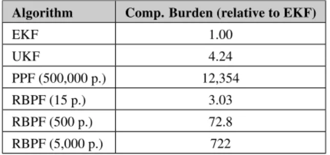
All simulations have been carried out using Matlab in a controlled Linux environment (ArchLinux distribution with 2.6.36 kernel) to ensure that the relative computational bur-den of each algorithm can be properly estimated. For the EKF, UKF and RBPF scenarios, 100 Monte Carlo simula-tions have been carried out spanning a time interval from 0s to 100s. For the PPF, only 15 Monte Carlo simulations have been performed because of the heavy computational burden and the available time. The ground-truth initial state vec-tor has been kept fixed and is given in Eq. 33 with SI units. For the Kalman filter-based simulations, the filter initial esti-mate has been set equal to the initial state vector plus a ran-dom vector in which each component was a ranran-dom Gaussian variable with zero mean and variance 0.1 (SI units). For the PF-based simulations, the initial value for each particle has been sampled from a uniform distribution, whose limits for the angles have been set from−45◦to+45◦, and−10◦/sto +10◦/sfor the angular rates.
x0=
25 −30 20 3 −3 −2 0 0 T· π
180 (33)
An unexpected, deterministic pulse disturbance torque has been applied at timet=45swith a 0.3sduration to inves-tigate filter robustness and convergence rate. The disturbing torque vector is given in Eq. 34.
Td,b=
−0.7 0.7 0.3 T N.m (34)
Table 1: Simulation parameters.
Symbol Description Value
General
∆ Sample time 0.01 s
τ Time constant of the low-pass filter in the RBPF
pseudo-measurement 0.2 s
Im,b Table inertia matrix, disregarding the reaction wheel, rep-resented in the table coordinate frame
0.4954/2 0.4954·0.1 −0.4954·0.1
0.4954·0.1 0.4954/2 0.4954·0.05 −0.4954·0.1 0.4954·0.05 0.4954
kg.m
2
Iw,b Reaction wheel inertia matrix represented in the table co-ordinate frame
1.5·10−3/2 1.5·10−3·0.1 −1.5·10−3·0.1 1.5·10−3·0.1 1.5·10−3/2 1.5·10−3·0.05 −1.5·10−3·0.1 1.5·10−3·0.05 1.5·10−3
kg.m
2
Bl Local magnetic field represented in the reference coordi-nate frame
h
0.8729 −0.4364 0.2182
iT
·500 mGauss
Sensors
εaccel Accelerometer bias 1 mg
σ2
accel Accelerometer measurement noise variance (0.002 √
30)2 (m/s2)2
σ2
tac Tachometer measurement noise variance 0.005 V2
σ2
mag Magnetometer measurement noise variance (0.5 √
10)2 (mGauss)2
Actuators
T pmax Pneumatic actuator maximum torque output 0.1 N·m
σ2
p Pneumatic actuator torque noise variance 10−4 (N·m)2 fp Pneumatic actuator PWM carrier frequency 2 Hz
ωwb
b,max Reaction wheel maximum angular rate 4,200 RPM Twmax Reaction wheel maximum torque 0.05 N·m
Km,w Reaction wheel motor constant 0.023 N·m/A ic,sat Reaction wheel current saturation Twmax/Km,w A Rm,w Reaction wheel motor resistance 10 Ω
Vc,sat Reaction wheel voltage saturation Rm,w·ic,sat V Kc,pi Proportional gain in reaction wheel PI controller 10 V/A
Ic,pi Integral gain in reaction wheel PI controller 2 V/(A·s)
Bw Reaction wheel viscous friction coefficient 4.9·10−6 N·m·s/rad
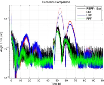
Eqs. 31-32 for each scenario have been plotted in Fig. 4. To improve the analysis, a zoom of the angular rate error norm in steady state has also been plotted in Fig. 5. The com-parison between EKF, UKF, PPF, and the proposed RBPF can be found in Fig. 6 and Fig. 7. Due to lack of space, additional results regarding the EKF, UKF and PPF can be found in Chagas and Waldmann (2010a) and Chagas and Waldmann (2010). Finally, Table 2 summarizes the com-putational burden results for each scenario. Figure 4 and Fig. 5 show that increasing the number of particles from 500 to 5,000 has not improved RBPF attitude estimation, but provided a slightly improved angular rate estimation in steady state. Figures 6 and 7 show that even with a very low number of particles, the RBPF achieved an attitude determi-nation accuracy that is comparable to the PPF with a huge number of particles. Furthermore, the angular rate estima-tion accuracy with just 15 particles is statistically the same as the PPF, but Kalman-based methods perform angular rate estimation better than the RBPF and PPF algorithms. The convergence rates of the PF-based estimation methods PPF and RBPF were better than that of the Kalman filter-based algorithms, with PPF yielding a slightly faster convergence than RBPF.
Table 2: Computational burden comparison.
Algorithm Comp. Burden (relative to EKF)
EKF 1.00
UKF 4.24
PPF (500,000 p.) 12,354
RBPF (15 p.) 3.03
RBPF (500 p.) 72.8
RBPF (5,000 p.) 722
6
CONCLUSIONS
A Rao-Blackwellized particle filter has been designed to es-timate satellite attitude and angular rate composed with a straightforward, linearized state feedback law for attitude control in a simulated, air-suspended table. The table uses two pneumatic actuators for alignment with the local hori-zontal plane, and one reaction wheel for azimuth alignment. The sensors consist of two accelerometers to estimate the lo-cal gravity vector direction, and two magnetometers - one on board the table, and the other fixed to the reference co-ordinate frame to provide azimuth alignment about the lo-cal vertilo-cal. The RBPF implementation proposed here for the particular application partitions the state-space into two groups: one formed by the attitude Euler angles and another with the angular rates. Particle sampling has been carried out just from the angular-rate subspace, whereas the Euler angles
were estimated by a set of Extended Kalman filters. For that purpose, approximations have been employed to decrease the computational burden and to render the problem analytically tractable. In such a case achieving the minimum mean square error estimate is not granted though when the number of par-ticles tends to infinity. Additionally, a significant reduction in the number of sampling particles has been accomplished by augmenting the measurement vector with low-pass filtering of the time-derivative of the vector observation. This aug-mented pseudo-measurement has guided the sampling of the angular-rate subspace, thus significantly decreasing the num-ber of particles needed while simultaneously maintaining es-timation accuracy.
The proposed RBPF yields a superior cost-benefit ratio than the PPF, because the former provided an estimation accuracy akin to the latter, and yet called for a much alleviated com-putational workload. However, by keeping a low number of particles the RBPF angular rate estimation accuracy has re-sulted inferior to those of the EKF or UKF. Moreover, both RBPF and PPF have produced attitude estimation far more robust to a torque disturbance. Therefore, when dealing with space applications that resort to sensors that measure vector observations and demand accurate angular rate control com-posed with the sound rejection of a disturbance torque - all of that without incurring in a heavy computational burden -, then the results reported here indeed encourage the use of the EKF or UKF running in parallel with the proposed RBPF with a small number of sampling particles.
Figure 4: Figures of Merit for RBPF using 15, 500 and 5000 particles.
Figure 5: Zoom of steady state angular rate estimation error for RBPF.
Since the computational load of the RBPF with 15 particles is only about 3 times higher than that of the usual EKF, and has a disturbance rejection very similar to the PPF, its implemen-tation has been considered feasible for this space application with adequate computational resources. Angular rate estima-tion quality can be improved with an architecture in which one EKF runs in parallel with the RBPF to accurately pro-vide, respectively, angular rate and attitude estimates. Even
Figure 6: Comparison between the proposed scenarios - Attitude determination.
Figure 7: Comparison between the proposed scenarios - Angular rate determination.
APPENDICES
A
PROOF OF EQUATION 19
Differentiating the first three measurement vector compo-nents with respect to time one gets Eq. A.1:
dy1 dt dy2
dt dy3
dt
=
−sin(θ)cos(φ)θ˙+cos(θ)cos(φ)φ˙ cos(θ)θ˙
sin(ψ)ψ˙
(A.1)
Equations 9 describe the kinematics relating the time deriva-tive of the Euler angles and the table angular rate vector with respect to the inertial frame. Equation 19 is proved by means of substituting the kinematics in the Eq. A.1 and writing in a compact matrix form.
B
PROOF OF THEOREM 1
Firstly, using Bayes rule and process model present at Eqs. 24, one can see that:
p(rk|z0:k,y0:k−1,yz,k) =
= p(zk|z0:k−1,y0:k−1,yz,k,rk)·p(rk|z0:k−1,y0:k−1,yz,k) p(zk|z0:k−1,y0:k−1,yz,k)
=
= p(zk|zk−1,yz,k)·p(rk|z0:k−1,y0:k−1,yz,k) p(zk|zk−1,yz,k)
=
=p(rk|z0:k−1,y0:k−1,yz,k)
(B.1)
Also:
p(yr,k|z0:k,y0:k−1,yz,k,rk) =p(yr,k|rk) =
=p(yr,k|z0:k−1,y0:k−1,yz,k,rk)
(B.2)
Applying the total probability theorem and using Eqs. B.1 and B.2:
p(yr,k|z0:k,y0:k−1,yz,k) =
=
Z
R3[p(yr,k|z0:k,y0:k−1,yz,k,rk)·
·p(rk|z0:k,y0:k−1,yz,k)]drk=
=
Z
R3[p(yr,k|z0:k−1,y0:k−1,yz,k,rk)·
·p(rk|z0:k−1,y0:k−1,yz,k)]drk=
=p(yr,k|z0:k−1,y0:k−1,yz,k)
(B.3)
Finally the theorem can be proved by applying Bayes rule to the importance density thus yielding:
p(zk|z0:k−1,y0:k) =p(zk|z0:k−1,yr,0:k,yz,0:k) =
= p(yr,k|z0:k,y0:k−1,yz,k)·p(zk|z0:k−1,y0:k−1,yz,k) p(yr,k|z0:k−1,y0:k−1,yz,k)
=
= p(yr,k|z0:k−1,y0:k−1,yz,k)·p(zk|z0:k−1,y0:k−1,yz,k) p(yr,k|z0:k−1,y0:k−1,yz,k)
=
=p(zk|z0:k−1,y0:k−1,yz,k) =p(zk|zk−1,yz,k)
(B.4)
C
PROOF OF THEOREM 2
For the optimal importance density, the weights are updated using (Doucet, 1998):
wkj=Ck−1·wkj−1·p(yk|z( j)
0:k−1,y0:k−1) (C.1) Firstly notice that, when conditioned onrk,yr,k is
indepen-dent ofyz,k. Hence:
p(yk|z(0:jk)−1,y0:k−1,rk) =p(yr,k,yz,k|z0:(jk)−1,y0:k−1,rk) =
=p(yz,k|z0:(jk)−1,y0:k−1,rk)·p(yr,k|z0:(jk)−1,y0:k−1,rk)
(C.2)
Also, using Bayes rule and process model present at Eqs. 24:
p(yz,k|z( j)
0:k−1,y0:k−1,rk) =
= p(rk|z (j)
0:k−1,y0:k−1,yz,k)·p(yz,k|z( j)
0:k−1,y0:k−1) p(rk|z0:(jk)−1,y0:k−1)
=
= p(rk|z (j)
0:k−1,y0:k−1)·p(yz,k|z(0:jk)−1,y0:k−1) p(rk|z0:(jk)−1,y0:k−1)
=
(C.3)
Using the total probability theorem in Eq. C.1:
wkj=Ck−1·wkj−1 Z
R3
h
p(yk|z(0:j)k−1,y0:k−1,rk)·
·p(rk|z0:(jk)−1,y0:k−1)
i
drk
(C.4)
Applying Eq. C.2 in Eq. C.4, one gets:
wkj=Ck−1·wkj−1 Z
R3
h
p(yz,k|z(0:jk)−1,y0:k−1,rk)·
·p(yr,k|z0:(j)k−1,y0:k−1,rk)·p(rk|z0:(j)k−1,y0:k−1)
i
drk
(C.5)
Finally, using Eq. C.3 in Eq. C.5:
wkj=Ck−1·wkj−1 Z
R3
h
p(yz,k|z0:(jk)−1,y0:k−1)·
·p(yr,k|z0:(j)k−1,y0:k−1,rk)·p(rk|z0:(j)k−1,y0:k−1)
i
drk
=Ck−1·wkj−1·p(yz,k|z(0:jk)−1,y0:k−1)·
·
Z
R3
h
p(yr,k|z( j)
0:k−1,y0:k−1,rk)·
·p(rk|z( j)
0:k−1,y0:k−1)
i
drk
=Ck−1·wkj−1·p(yz,k|z( j)
0:k−1,y0:k−1)·
·
Z
R3
h
p(yr,k|rk)·p(rk|z(0:j)k−1,y0:k−1)
i
drk
(C.6)
Doucet (1998) showed that:
p(yz,k|z( j)
0:k−1,y0:k−1) =p(yz,k|z( j)
k−1) = =N(yz,k;Hzfz(z(
j)
k−1,uk−1),HzQzHTz +Rz)
(C.7)
Also, the P.D.F p(rk|z( j)
0:k−1,y0:k−1)is approximated by a Gaussian density with mean and covariance computed by the set of extended Kalman filters:
p(rk|z(0:jk)−1,y0:k−1)≈N(rk; ˆr(k|jk)−1,P(k|jk)−1) (C.8)
It can be easily seen that:
p(yr,k|rk) =N(yr,k;hr(rk),Rr) (C.9)
Using this formulation, the integral in Eq. C.6 cannot be an-alytically solved due to the nonlinear functionhr(rk). To
cir-cumvent this problem, this function is linearized about ˆr(k|jk)−1 as follows:
hr(rk)≈hr(rˆ( j)
k|k−1) +H (j)
r,k·(rk−rˆ( j)
k|k−1) (C.10)
whereH(r,jk)= ∂hr(r) ∂r
r=ˆr(j)
k|k−1
. Hence, the P.D.F. expressed in
Eq. C.9 can be approximated by:
p(yr,k|rk) =N(yr,k;hr(rk),Rr) =
=Ξ·exp
−1
2(yr,k−hr(rk))
T
R−r1(yr,k−hr(rk))
≈
≈Ξ·exp
−1
2
yr,k−hr(rˆk(|jk)−1)−Hr(,jk)·(rk−rˆ(k|jk)−1) T
·
·R−r1yr,k−hr(ˆr(k|jk)−1)−H(r,jk)·(rk−rˆ(k|jk)−1)
=
=Ξ·exp
−1
2
˜ yr,k−H(
j)
r,krk T
R−r1
˜ yr,k−H(
j)
r,krk
=
=N(y˜r,k;H(r,kj)rk,Rr)
(C.11)
where y˜r,k=yr,k−hr(rˆk(j|k)−1) +H(r,jk)rˆ
(j)
k|k−1 and
Ξ= (2π)3·det(R
r) −12
.
Therefore, using Eq. C.7, Eq. C.8, Eq. C.9, and Eq. C.11, the weights calculations in Eq. C.6 can be approximated by:
wkj≈Ck−1·wkj−1·
·N(yz,k;Hzfz(z( j)
k−1,uk−1),HzQzHTz +Rz)·
·
Z
R3N(y˜r,k;H (j)
r,krk,Rr)·N(rk; ˆrk(|jk)−1,Pk(|jk)−1)drk
(C.12)
With this approximation, the aforementioned integral can be evaluated. Firstly, one should consider the Chapman-Kolmogorov equation applied to the prediction step of the standard Kalman filter, shown in Eq. C.13 (Arulampalam et al., 2002):
p(xk|y0:k−1) =
=
Z
Rnp(xk|xk−1,y0:k−1)·p(xk−1|y0:k−1)dxk−1
=
Z
Rnp(xk|xk−1)·p(xk−1|y0:k−1)dxk−1
(C.13)
Both P.D.F. in the above integral are rewritten in the standard linear Kalman filter problem as follows (Ho and Lee, 1964; Anderson and Moore, 1979):
Z
RnN(xk;Fkxk−1,Qk)·N(xk−1; ˆxk−1|k−1,Pk−1|k−1)dxk−1=
=N(xk;Fkxˆk−1|k−1,FkPk−1|k−1FTk+Qk)
(C.14)
Performing the following variable substitution in Eq. C.14:
xk→y˜r,k, Fk→H( j)
r,k, xk−1→rk, Qk→Rr,
ˆ
xk−1|k−1→rˆ (j)
k|k−1, Pk−1|k−1→P (j)