Copyright © 2010 SBMAC ISSN 0101-8205
www.scielo.br/cam
Preconditioners for higher order finite element
discretizations of
H
(
div
)
-elliptic problem
JUNXIAN WANG, LIUQIANG ZHONG and SHI SHU School of Mathematical and Computational Sciences,
Xiangtan University, Hunan 411105, China
E-mails: [email protected] / [email protected] / [email protected]
Abstract. In this paper, we are concerned with the fast solvers for higher order finite element
discretizations of H(div)-elliptic problem. We present the preconditioners for the first family and second family of higher order divergence conforming element equations, respectively. By combining the stable decompositions of two kinds of finite element spaces with the abstract theory of auxiliary space preconditioning, we prove that the corresponding condition numbers of our preconditioners are uniformly bounded on quasi-uniform grids.
Mathematical subject classification: Primary: 65F10; Secondary: 65N22.
Key words: preconditioner, higher order finite element, stable decomposition,H(div)-elliptic
problem.
1 Introduction
Letbe a simply connected polyhedron inR3with boundaryŴand unit outward
normalν. We define the Hilbert spacesH0(div;)as follows
H0(div;) = u∈(L2())3 ∇ ∙u∈ L2(), ν∙u=0 onŴ with the inner product
(u,v)div =(u,v)+(∇ ∙u,∇ ∙v),
where(∙,∙)denotes the inner product in(L2())3orL2().
In this paper, we consider the following variational problem: Find
u∈ H0(div;)such that
a(u,v)=(f,v) ∀v ∈ H0(div;), (1)
where f ∈ H0(div;)′is a given data and
a(u,v)=(∇ ∙u,∇ ∙v)+τ (u,v), (2)
with the constantτ >0.
The bilinear forma(∙,∙)induces the energy norm
kvk2A=a(v,v) ∀v∈ H0(div;). (3) Variational problem of the form (1) arises in numerous problems of practi-cal import. Typipracti-cal examples include the mixed method for second order elliptic problems, the least squares method of the form discussed in [3], and the sequential regularization method for the time dependent Navier-Stokes equation discussed in [6]. For a more detailed discussion of applications, we refer to [1].
To avoid the repeated use of generic but unspecified constants, following [9],
we will use the following short notation: x . ymeansx ≤C y,x & y means
x ≥ cy, andx ≈ y meanscx ≤ y ≤ C y, wherec andC are generic positive
constants independent of the variables that appear in the inequalities and espe-cially the mesh parameters.
Outline. The remainder of this article is organized as follows. In the next section, we introduce two kinds of higher order finite element equations, and present the corresponding frame of constructing preconditioner. We construct the preconditioners for two kinds of higher order divergence conforming element equations, and prove that their corresponding condition number is uniformly bounded in Section 3 and Section 4, respectively.
2 Finite element equations and framework of preconditioner
LetTh be a shape regular tetrahedron meshes of , where h is the maximum
conforming finite elements spaces (see [7])
Wkh,1=
n
vkh,1∈ H0(div;)
v
k,1
h |K ∈(Pk−1)3⊕ ˜Pk−1x,∀K ∈Th o
,
Wkh,2=
n
vkh,2∈ H0(div;)
v
k,2
h |K ∈(Pk)3,∀K ∈Th o
,
wherePk denote the standard space of polynomials of total degree less than or
equal tok, andP˜k denote the space of homogeneous polynomials of orderk.
We consider the solution of systems of linear algebraic equations which arise
from the finite element discretization of variational problems (1): Find
ukh,l ∈Wkh,l(k≥1,l =1,2)such that
a(ukh,l,vkh,l)=(f,vhk,l) ∀vhk,l ∈Wkh,l. (4)
Their algebraic systems can be described as
Akh,lUhk,l =Fhk,l. (5)
Since Akh,l is symmetric positive definite, we use precondition conjugate gra-dient (PCG) methods to solve algebraic systems (5). In this paper, we will construct the preconditioners for the cases of higher order finite equations, and present some estimates of the corresponding condition numbers.
For this purpose, we need to introduce some auxiliary spaces and corre-sponding operators.
LetV =Wkh,l with inner producta(∙,∙)given by (2).
Let Vˉ1,∙ ∙ ∙,VˉJ,J ∈ N, be Hilbert spaces endowed with inner products
ˉ
aj(∙,∙),j = 1,∙ ∙ ∙,J. The operators Aˉj : ˉVj 7→ ˉVj′ are isomorphisms in-duced byaˉj(∙,∙), namely
ˉ
aj(uˉj,vˉj)=< Aˉjuˉj,vˉj > ∀ ˉuj,vˉj ∈ ˉVj,
here we tag dual spaces by′ and use angle brackets for duality pairings. For
eachVˉj, there exist continuous transfer operators5j : ˉVj 7→ V. Then we can construct the preconditioner for operator Akh,l as follows:
B =
J X
j=1
where Bˉj : ˉVj′ 7→ ˉVj are given preconditioners for Aˉj, and 5∗j are adjoint operators of5j.
Now, we present the following theorem of an estimate for the spectral condition number of the preconditioner given by (6).
Theorem 2.1. Assume that there exist constants cj, such that
k5juˉjkA ≤cjk ˉujkAˉj, ∀ ˉuj ∈ ˉVj, 1≤ j ≤ J, (7)
and for∀u∈ V , there existuˉj ∈ ˉVj such that u= PJ
j=15juˉj and
J X
j=1
k ˉujk2Aˉj
1/2
≤c0kukA, (8)
then for the preconditioner B given by (6), we have the following estimate for the spectral condition number
κ(B Akh,l)≤ max
1≤j≤Jκ(
ˉ
BjAˉj)c20
J X
j=1
c2j. (9)
Proof. We define the space
ˉ
V = ˉV1× ˉV2× ∙ ∙ ∙ × ˉVJ with the inner product
(uˉ,uˉ)Aˉ =
J X
j=1
(uˉj,uˉj)Aˉj,uˉ =(uˉ1,uˉ2,∙ ∙ ∙,uˉJ)t,uˉi ∈ ˉVj,
and the following two operators
5=(51, 52,∙ ∙ ∙, 5J): ˉV 7→V,
ˉ
A=diag(Aˉ1,Aˉ2,∙ ∙ ∙,AˉJ): ˉV 7→ ˉV,
ˉ
B =diag(Bˉ1,Bˉ2,∙ ∙ ∙ ,BˉJ): ˉV 7→ ˉV.
Thus we can rewrite the definition of operatorB given by (6):
Using the definitions of inner product inVˉ, operators5andBˉ, and conditions (7)-(8), then there exists a constantcˉ2
1:=
PJ j=1c
2
j, such that
k5uˉkA≤ ˉc1k ˉukAˉ, ∀ ˉu ∈ ˉV,
and for∀u∈ V, there existsuˉ ∈ ˉV, such thatu=5uˉ and
k ˉukAˉ ≤c0kukA.
From Corollary 2.3 of [5], we immediately get an estimate for the spectral
condition number of the preconditioned operator B
κ(B Akh,l)≤κ(BˉAˉ)c20
J X
j=1
c2j.
The desired estimates then follow by combining the above inequality and the following fact
κ(BˉAˉ)≤ max
1≤j≤Jκ(
ˉ
BjAˉj).
The principal challenge confronted in the development of preconditioners by applying Theorem 2.1 is to construct some appropriate spaces and operators which satisfy (7) and (8). In the following two sections, we present the corre-sponding spaces and operators for two kinds of divergence conforming element spaces, respectively.
3 Preconditioner for finite element equations of first kind
We first introduce Sobolev functional space
H0(curl;)=
u∈(L2())3∇ ×u∈(L2())3,ν×u=0onŴ with the norm
kukH(curl;)= kuk20+ k∇ ×uk 2 0
1/2
.
There exist two families of edge finite element spaces for the space
1. korder Nédélec element of first kind:
Vkh,1=
n
ukh,1∈ H0(curl;)
u
k,1
h |K ∈Rk,∀K ∈Th o
, (10)
whereRk =(Pk−1)3⊕ {p∈(P˜k)3| p(x)·x=0}.
2. korder Nédélec element of second kind:
Vkh,2=
n
ukh,2∈ H0(curl;)
u
k,2
h |K ∈(Pk)3,∀K ∈Th o
. (11)
We also need to introduce the following space of piecewisek−degree
discon-tinuous scalar elements onTh:
Xkh=nqhk ∈ L2()
q
k
h|K ∈Pk for all K ∈Th o
.
The Sobolev spaces H0(div;), H0(curl;)and the corresponding finite
element spaces possess the exceptional exact sequence properties (see [4, 7])
H0(div0;) := {w∈ H0(div;): ∇ ∙w=0}
= ∇ × H0(curl;), (12)
Wkh−1,l(div0) := {wkh−1,l ∈Whk−1,l : ∇ ∙whk−1,l =0}
= ∇ ×Vkh,l, l=1,2, (13)
∇ ∙Wkh,l ⊂ Xhk−1, l =1,2. (14)
Assuming that u has the necessary smoothness, we can define two kinds of
interpolants: 5kh,,1div and 5kh, such that 5hk,,1divu ∈ Wkh,1 and5khu ∈ Xkh (more details refer to [4, 7]). Especially, the interpolation5kh,,1div is not defined for a general function in H0(div;). Here let us quote a slightly simplified version (see Theorem 5.25 of [7]).
Lemma 3.1. Suppose that there are constants δ > 0 such that u ∈
(H1/2+δ(K))3for each K inT
h. Then5kh,,1divuis well-defined, and we have
The finite element spaces Wkh,1 is equipped with bases B(k,1) comprising locally supported functions. These bases areL2stable in the sense that
vkh,1= X
b∈B(k,1)
vb, vb∈span{b},
X
b∈B(k,1)
kvbk20≈kv
k,1
h k
2 0∀v
k,1
h ∈ W k,1
h , (16)
with constant only depending on the shape-regularity ofTh.
Lemma 3.2. The interpolation operator 5kh,,1div is bounded on(H01())3 and
satisfies
k(I d−5hk,,1div)ψk0.hkψk(H1())3 ∀ψ ∈(H01())3 (17) with a constant only depending on the shape regularity ofTh.
Furthermore, all above operators possess the following commuting diagram property (see [7])
div5kh,,1div = 5kh−1div. (18)
We may apply the quasi-interpolation operators for Lagrangian finite element space introduced in [8] to the components of vector fields separately. This gives rise to the projectorsQh:(H01())37→(Sh1)3, which inherits the continuity
kQh9k(H1())3 .k9k(H1())3 ∀9 ∈(H01())3 (19)
and satisfies the local projection error esitmate
kh−1(I d−Qh)9k0.k9k(H1())3 ∀9 ∈(H01())3. (20)
Now, we present the stable decomposition ofWkh,1,k≥2. Lemma 3.3. For any ukh,1 ∈ Wkh,1, there exist P
b∈B(k,1)vb ∈ Wkh,1,vb ∈
Span{b},uhk−1,2∈Wkh−1,2,such that
ukh,1= X
b∈B(k,1)
vb+u k−1,2
h , (21)
and
X
b∈B(k,1)
kvbk2A+ ku k−1,2
h k
2
A
1/2
where the constantc˜0only depends onand the shape regularity ofTh. Proof. For any givenukh,1∈ Wkh,1, using the continuous Helmholtz decomposi-tion, there exist9 ∈(H1
0())3,p∈ H0(curl;)such that
ukh,1=9 + ∇ × p, (23) and
k9k(H1())3 .k∇ ∙ukh,1k0, k∇ × pk0.kuhk,1kH(div;), (24)
with constants only depending on.
Taking the div of both sides of (23) and using (14), we get
∇ ∙9 = ∇ ∙ukh,1∈ Xkh−1.
Owing to Lemma 3.2,5kh,,1div9 is well defined. Furthermore, the commuting diagram property (18) implies
∇ ∙5kh,,1div9 =5kh−1∇ ∙9 = ∇ ∙9 ⇒ ∇ ∙(I d−5kh,,1div)9 =0.
This confirms that the third term in the splitting
9 =5kh,,1div(I d−Qh)9+5kh,,1divQh9 +(I d−5kh,,1div)9 (25) actually belongs to the kernel of div. By (12), then there esistsq ∈ H0(curl;)
such that
(I d−5kh,,1div)9 = ∇ ×q. (26) Noting thatQh9 ∈(Sh1)
3⊂Wk,1
h , which leads to
5kh,,1divQh9 =Qh9. (27) Substituting (25), (26) and (27) into (23), we have
ukh,1=5kh,,1div(I d−Qh)9+Qh9 + ∇ ×(q+ p). (28) Since ukh,1, 5hk,,1div(I d − Qh)9,Qh9 ∈ Wkh,1, we obtain ∇ × (q + p) ∈
Wkh,1(div0) by using (28), then observing (13), there exists qh ∈ V k,1
h , such
that
Let
˜
ukh,1 = 5hk,,1div(I d−Qh)9 = X
b∈B(k,1)
vb,vb ∈Span{b}, (30)
ukh−1,2 = Qh9+ ∇ ×qh. (31) It’s easy to obtainukh−1,2∈Whk−1,2by noting thatQh9 ∈(Sh1)
3⊂Wk−1,2
h and
∇ ×qh ∈ ∇ ×V k,1
h ⊂ W k−1,2
h . Substituting (29), (30) and (31) into (28), we
conclude
ukh,1= X
b∈B(k,1)
vb+ukh−1,2, (32)
which completes the proof of (21).
Using (30), triangular inequality, Lemma 3.2, (20) and (24), we have
kh−1u˜kh,1k0 = kh−15kh,,1div(I d−Qh)9k0
≤ kh−1(I d−5kh,,1div)(I d−Qh)9k0+ kh−1(I d−Qh)9k0
. k(I d−Qh)9k(H1())3+ k9k(H1())3
. k9k(H1())3 .k∇ ∙ukh,1k0,
which leads to
k ˜ukh,1k0 . hk∇ ∙ukh,1k0. (33)
It follows readily from inverse estimate and (16) that
X
b∈B(k,1)
kvbk2A = X
b∈B(k,1)
k∇ ∙vbk20+τkvbk20
. X
b∈B(k,1)
kh−1vbk02+τkvbk20
. h−2+τk ˜uhk,1k20. (34) Using inverse estimate again yields
By means of (33) and inverse estimate, we get
h−2+τk ˜ukh,1k20 . h−2+τh2k∇ ∙ukh,1k20
. k∇ ∙ukh,1k20+τkukh,1k20
= kukh,1k2A. (36) In view of (32), triangular inequality (34), (35) and (36), we have
X
b∈B(k,1)
kvbk2A+ ku k−1,2
h k
2
A ≤ X
b∈B(k,1)
kvbk2A+
kukh,1kA+ k ˜ukh,1kA 2
. h−2+τk ˜uhk,1k20+ kukh,1k2A
. kukh,1k2A,
which completes the proof of (22).
We rely on the stable decomposition forV = Wkh,1in Lemma 3.3 and apply
the abstract theory in Section 2 to define the preconditioner for finite element equations of first kind.
LetV =Wkh,1and choose two auxiliary spaces and the corresponding transfer operators as follows.
1. Vˉ1=Whk,1, with inner productaˉ1(∙,∙)which is defined by
ˉ
a1(uˉ1,v1)ˉ :=< Aˉ1uˉ1,v1ˉ >=
X
b∈B(k,1)
a(ub,vb),
where
ˉ
u1=
X
b∈B(k,1)
ub,vˉ1=
X
b∈B(k,1)
vb,ub,vb ∈span{b}.
The transfer operator is51= I d.
2. Vˉ2=Wkh−1,2with inner productaˉ2(∙,∙)=a(∙,∙)in the sense that
ˉ
a2(uˉ2,vˉ2):=< Aˉ2uˉ2,vˉ2>=a(uˉ2,vˉ2) ∀ ˉu2,vˉ2∈ ˉV2,
Making use of (6), the auxiliary space preconditioner for Akh,1reads Bhk,1= ˉB1+B
k−1,2
h , (37)
whereBhk−1,2is the preconditioner of Ahk−1,2, Bˉ1is the preconditioners of Aˉ1.
Noting thatAˉ1denotes the diagonal matrix ofAkh,1, in the practical application, we will take Bˉ1 as the Jacobi (or Gauss-Seidel) smoothing operator for Akh,1. Obviously, this special choose satisfies
κ(Bˉ1Aˉ1)≤ ˜C1, (38)
where the constantC˜1is independent of the mesh parameters.
First, we prove that the above transfer operators satisfy the condition (7). Due to the definitions of inner product and transfer operator in spaceVˉ1, for
any givenuˉ1=
P
b∈B(k,1)αbb∈ ˉV1, whereαb ∈R, we have
k51uˉ1k2A = k ˉu1k2A = X
b∈B(k,1)
αbb
2 A = X
K∈Th
M X
j=1 αbb
2
A,K
≤ M X
K∈Th
X
b∈B(k,1)
kαbbk2A,K = Mk ˉu1k2Aˉ1, (39)
where the constant M bounds the number of basis functions whose support
overlaps with a single elementK.
For any givenuˉ2∈ ˉV2,it’s easy to obain
k52uˉ2kA = k ˉu2kA = k ˉu2kAˉ2. (40)
Combining (39) with (40), we conclude that (7) holds with the constantsc1=
Mandc2=1.
Secondly, the above spaces and operators satisfy the condition (8) by using the Lemma 3.3.
Summing up, we obtain the following theorem by using Theorem 2.1.
Theorem 3.4. For Bhk,1 given by(37), and Bˉ1 satisfies the condition of (38),
then we have
κ(Bhk,1Akh,1).κ(Bhk−1,2Akh−1,2), (41) with a constant only depending on the constantsc˜0,C˜1and the shape regularity
4 Preconditioner for finite element equations of second kind
Now, we present the another stable decomposition ofWkh−1,2withk ≥2. Lemma 4.1.For anyukh−1,2∈Wkh−1,2, there areuhk−1,1∈Whk−1,1andϕh ∈ V
k,2
h
such that
uhk−1,2=uhk−1,1+ ∇ ×ϕh, (42)
and
kukh−1,1k2A+ k∇ ×ϕhk
2
A 1/2
≤c0kuk −1,2
h kA, (43)
where the constant c0only depends onand the shape regularity ofTh. Proof. For anyukh−1,2∈Wkh−1,2, we can interpolateukh−1,2by Lemma 3.1. Thus, using (18), we have
∇ ∙5hk−,div1,1ukh−1,2=5 k−2
h ∇ ∙u k−1,2
h . (44)
In view of (14), we have
∇ ∙ukh−1,2∈ X k−2
h . (45)
Making use of (45) and noting that5kh−2|Xk−2
h =I din (44), we get
∇ ∙5kh−,div1,1uhk−1,2= ∇ ∙ukh−1,2,
namely
∇ ∙
uhk−1,2−5kh−,div1,1ukh−1,2
=0. (46)
Noting that ukh−1,2 −5hk−,div1,1uhk−1,2 ∈ Wkh−1,2, then by (46) and (13), there existsϕh∈ Vkh,2,such that
Using (47), (15) withδ =1/2, and the inverse estimate, we obtain
k∇ ×ϕhk0,K = kukh−1,2−5 k−1,1
h,div u
k−1,2
h k0,K . hkukh−1,2k(H1(K))3 .kukh−1,2k0,K. Squaring and summing over all the elements, we get
k∇ ×ϕhk20 =
X
K∈Th
k∇ ×ϕhk20,K
. X
K∈Th
kukh−1,2k20,K = kukh−1,2k20. (48)
In view of (3) and (48), we find
k∇ ×ϕhk2A =τk∇ ×ϕhk20.τku
k−1,2
h k
2 0≤ ku
k−1,2
h k
2
A. (49)
Making use of (47), triangular inequality and (48), we have
kukh−1,1k0≤ kuhk−1,2k0+ k∇ ×ϕhk0.kukh−1,2k
2
0. (50)
A direct manipulation of (47) gives that
k∇ ∙ukh−1,1k0= k∇ ∙ukh−1,2k0. (51)
A combination of (49), (50) and (51) concludes (43).
In this case, let V = Wkh−1,2. We choose the following two auxiliary spaces and the corresponding transfer operator.
1. Vˉ1=Wkh−1,1with inner productaˉ1(∙,∙)=a(∙,∙)in the sense that
ˉ
a1(uˉ1,v1)ˉ :=< Aˉ1uˉ1,v1ˉ >=a(uˉ1,v1)ˉ ∀ ˉu1,v1ˉ ∈ ˉV1,
which concludes that Aˉ1 = A
k−1,1
h . The corresponding transfer operator
is51= I d.
2. Vˉ2=V
k,2
h with inner product
ˉ
a2(uˉ2,vˉ2):=< Aˉ2uˉ2,vˉ2>=τ (∇ × ˉu2,∇ × ˉv2) ∀ ˉu2,vˉ2∈ ˉV2. (52)
Then by using (6), we obtain the auxiliary space preconditioner for Akh−1,2as follows
Bhk−1,2 =Bhk−1,1+curlBˉ2curl∗, (53)
where Bhk−1,1 is the preconditioner of Ahk−1,1, and Bˉ2 is the preconditioners of
ˉ
A2given by (52).
Especially, we adopt the preconditioner Bˉ2in [10], this choice satisfy
κ(Bˉ2Aˉ2)≤C1, (54)
where the constantC1is independent of the mesh parameters.
It is easy to prove that the above transfer operators satisfy the conditions (7). In fact, using the definitions of inner products and transfer operators in spaces
ˉ
Vl(l=1,2), we have
k51vˉ1kA= k ˉv1kA = k ˉv1kAˉ1, ∀ ˉv1∈ ˉV1, (55)
k52vˉ2k2A = k∇ × ˉv2k2A=τk∇ × ˉv2k20= k ˉv2k2Aˉ2,∀ ˉv2∈ ˉV2, (56)
namely, the conditions (7) of Theorem 2.1 hold with the constantsc1=c2=1.
Applying Theorem 2.1 and using Lemma 4.1, we have the following Theorem.
Theorem 4.2. For Bhk−1,2 given by (53), and Bˉ2 satisfies the condition of (54), then we have
κ(Bhk−1,2Akh−1,2).κ(Bhk−1,1Akh−1,1), (57) with a constant only depending on the constants c0and C1and the shape
regu-larity ofTh.
Combining Theorem 3.4 and Theorem 4.2, by using a Jacobi (or Gauss-Seidel) smoothing, we can translate the construction of preconditioner forAkh,1into the one of Akh−1,2. Furthermore, by using the preconditioner of H(curl;)-elliptic problem, we can translate the preconditioner for Akh−1,2into the one for Akh−1,1.
Since Hiptmair and Xu [5] have constructed an efficient preconditioner Bh1,1
for A1h,1, we construct the efficient precondtioners for Ahk,l(k = 1, l =
2 ork ≥ 2,l =1,2)and prove the corresponding spectral condition numbers
are uniformly bounded and independent of mesh sizeh and the parameterτ by
5 Implementation of algorithm and numerical experiments
For simplicity, we only give the description of the preconditioning algorithm
defined by (53) whenk =2.
Note that whenk =2, (53) turn to
Bh1,2= Bh1,1+curlBˉ2curl∗. (58)
In the following, we first discuss the description of algorithm about the pre-conditioner Bh1,1. For this purpose, we introduce the following operators
Pdc :W1,1−→ ∇ ×V1,1,
Pds :W1,1−→(Sh1)3,
Pcs :V
1,1
−→(Sh1)
3 ,
and
Ac1,1=PdcAh1,1(Pdc)T,
Ads = PdsAh1,1(Pds)T,
Acs = PcsAc1,1(Pcs)T,
then, the algorithm about the operator Bh1,1 can be described by (see [5] for more details)
Algorithm 5.1.For a given g∈W1h,1, then ug =Bh1,1g∈W1h,1can be obtained
as follows:
Step 1: Applying m1 times symmetric Gauss_Seidel iterations in variational
problem
a(u˜1,vh1,1)=(f,v
1,1
h ) ∀v
1,1
h ∈W
1,1
h
with a zero initial guess to getu˜1, where f =g.
Step 2: Computingu˜2∈(Sh1)3by
(Asdu˜2, v2)=(g, v2), ∀v2∈(Sh1)
Step 3: Computingu˜3∈ V1h,1by
(A1c,1u˜3,v˜3)=(g,∇ × ˜v3), ∀ ˜v3∈ V1h,1, (59)
which can be obtained by
1. Applying m2times symmetric Gauss_Seidel iterations in(59)with a
zero initial guess to getu˜4.
2. Computingu˜5∈(Sh1)
3by
(Ascu˜5, v5)=(g, v5), ∀v5∈(Sh1)
3
. (60)
3. Setu˜3= ˜u4+(Pcs)Tu˜5.
Step 4: Set ug= ˜u1+(Pds) Tu˜
2+(Pdc) Tu˜
3.
By [5], the preconditionerBh1,1defined by Algorithm 5.1 satisfy
κ(Bh1,1A1h,1)≤C1,
where the constantC1is independent of the mesh sizeh and parameterτ.
Next, we give the description of algorithm for the operator curlBˉ2curl∗.
Firstly, let
n=di m(V2h,1), m=di m(W
1,2
h ),
and
V2,1=span{φi,i =1,∙ ∙ ∙,n}, W1,2=span{ψj, j=1,∙ ∙ ∙ ,m}, then we introduce the transfer matrix(or operator) Pdc,2
∇ ×φ1
∇ ×φ2 .. .
∇ ×φn
= Pdc,2 ψ1 ψ2 .. . ψm ,
In view of (4.1) in [10], we can construct the preconditioner Bˉ2for A2c,1, and its spectral condition number satisfy
κ(Bˉ2A2c,1)≤C2,
where the constantC2is independent of the mesh sizeh and parameterτ.
Noting that the operator Bˉ2can be divided into three parts: the first part is to
use the Jacobi (or Gauss-Seidel) smoothing for (52) in spaceV2h,1, the second part is to solve the restriction of (52) in(Sh1)3, the third part is to solve the restriction of (52) in∇S2
h. We can drop the second and third parts by using the fact that
the second part is the same as (60) andcurl◦grad ≡ 0. Hence the operator
curlBˉ2curl∗can be simplified.
Summing up, we can obtain the following algorithm of the preconditionerBh1,2. Algorithm 5.2.For g∈ W1h,2, the solution ug =Bh1,2g ∈W
1,2
h can be gotten as
follows:
Step 1: Computing u1∈ W1h,1by Algorithm 5.1.
Step 2: Applying m3times symmetric Gauss_Seidel iterations to get u2 ∈V2,1
by
(A2c,1u2, v2)=(g,∇ ×v2), ∀v2∈V2,1.
Step 3: Set
ug=u1+u2.
For variational problem (4), we apply Algorithm 5.2 to the following two examples:
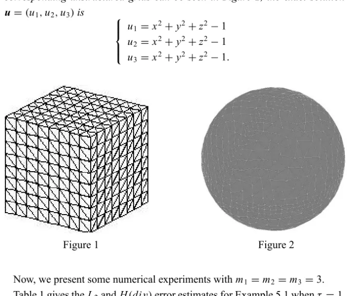
Example 5.1.The computational domain is= [0,1] × [0,1] × [0,1]and the corresponding structured grids can be seen in Figure 1. For the convenience of computing the exact errors, we construct an exact solutionu=(u1,u2,u3)as
u1=x yz(x−1)(y−1)(z−1)
u2=sin(πx)sin(πy)sin(πz)
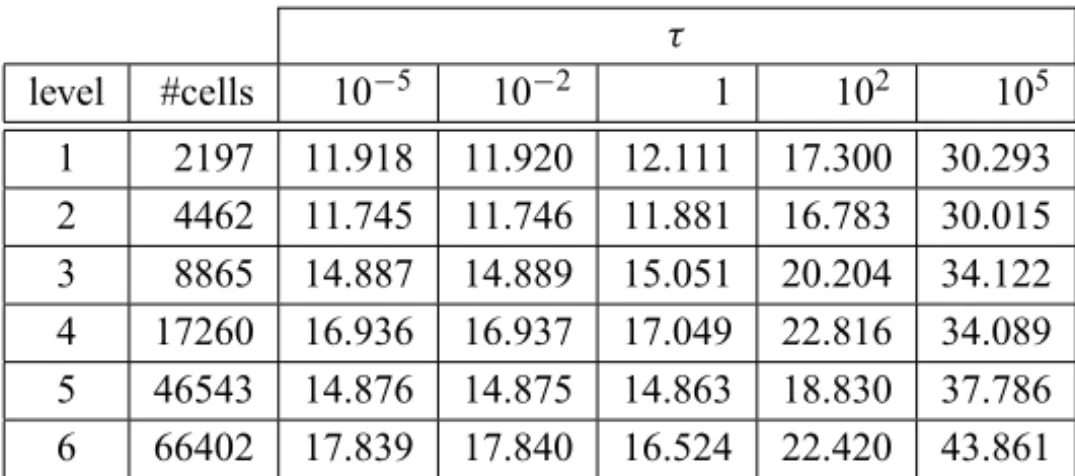
Example 5.2. The computational domain is the spheres of radius 1 and the corresponding unstructured grids can be seen in Figure 2, the exact solution
u=(u1,u2,u3)is
u1=x2+y2+z2−1
u2=x2+y2+z2−1
u3=x2+y2+z2−1.
Figure 1 Figure 2
Now, we present some numerical experiments withm1=m2=m3=3.
Table 1 gives theL2andH(div)error estimates for Example 5.1 whenτ =1,
which shows thatu1h,2is the optimal convergence.
Th iter ku−u1h,2kL2err rate ku−u1h,2kH(div)err rate
63 20 2.051e-2 2.040e-1
123 19 4.685e-3 4.378 1.026e-1 1.988
243 19 1.139e-3 4.113 5.141e-2 1.996
Table 1
The condition number estimates and iteration counts for Example 5.1 and Example 5.2 are listed in Tables 2 – 5 for different values of the mesh sizehand
the scaling parameterτ. By these Tables, we find that the condition number and
iteration counts are independent of the mesh sizehand weakly dependent on the
τ
level #cells 10−5 10−2 1 102 105 1 6×63 9.577 9.578 10.008 13.282 21.403 2 6×123 10.258 10.261 10.254 12.363 19.396 3 6×243 10.301 10.291 10.294 11.030 18.098
Table 2 – Unit cube: spectral condition number ofBh1,2A1h,2.
τ
level #cells 10−5 10−2 1 102 105
1 6×63 19 19 20 22 28
2 6×123 19 18 19 21 25
3 6×243 19 18 19 19 23
Table 3 – Number of PCG-iterations on unit cube.
τ
level #cells 10−5 10−2 1 102 105 1 2197 11.918 11.920 12.111 17.300 30.293 2 4462 11.745 11.746 11.881 16.783 30.015 3 8865 14.887 14.889 15.051 20.204 34.122 4 17260 16.936 16.937 17.049 22.816 34.089 5 46543 14.876 14.875 14.863 18.830 37.786 6 66402 17.839 17.840 16.524 22.420 43.861 Table 4 – Unit ball: spectral condition number ofBh1,2A1h,2.
τ
level #cells 10−5 10−2 1 102 105
1 2197 13 17 20 24 30
2 4462 13 17 20 24 30
3 8865 14 17 21 25 31
4 17260 14 17 20 23 29
5 46543 15 17 20 23 28
6 66402 16 17 20 23 27
Acknowledgements. The authors are partially supported by the National Natural Science Foundation of China (Grant No. 10771178), NSAF (Grant No. 10676031), the National Basic Research Program of China (973 Program) (Grant No. 2005CB321702). Especially, the first author is supported by Hunan Provincial Innovation Foundation For Postgraduate (Grant No. CX2009B121).
REFERENCES
[1] D.N. Arnold, R.S. Falk and R Winther, Preconditioning in H(div)and applications, Math. Comp.,66(1997), 957–984.
[2] A. Bossavit,Computational Electromagnetism. Variational Formulation, Complementarity, Edge Elments. San Diego: Academic Press (1998).
[3] Z. Cai, R. Lazarov, T. Manteuffel and S. McCormick, First-order system least squares for second-order partial differential equations: Part I, SIAM J. Numer. Anal.,31(1994), 1785–1799.
[4] R. Hiptmair, Finite elements in computational electromagnetism, Acta Numer.,11(2002), 237–339.
[5] R. Hiptmair and J. Xu,Nodal auxiliary space preconditioning in H(curl)and H(div)spaces, SIAM J. Numer. Anal.,45(2007), 2483–2509.
[6] P. Lin,A sequential regularization method for time-dependent incompressible Navier-Stokes equations, SIAM J. Numer. Anal.,34(1997), 1051–1071.
[7] P. Monk,Finite Element Methods for Maxwell Equations. Oxford University Press, Oxford (2003).
[8] L. R. Scott and S. Zhang, Finite element interpolation of nonsmooth functions satisfying boundary conditions, Math. Comp.,54(1990), 483–493.
[9] J. Xu, Iterative methods by space decomposition and subspace correction, SIAM Review,
34(1992), 581–613.