ISSN 0101-8205 www.scielo.br/cam
An explicit formulation for the inverse transport
problem using only external detectors – Part II:
Application to one-dimensional homogeneous and
heterogeneous participating media
NANCY I. ALVAREZ ACEVEDO1∗
, NILSON COSTA ROBERTY2
and ANTÔNIO J. SILVA NETO1
1Department of Mechanical Engineering and Energy, Instituto Politécnico, IPRJ
Universidade do Estado do Rio de Janeiro, UERJ P.O. Box 97282, 28601-970 Nova Friburgo, RJ, Brazil
2Nuclear Engineering Program, PEN/COPPE, Universidade Federal do Rio de Janeiro, UFRJ,
P.O. Box 68509, 21945-970 Rio de Janeiro, RJ, Brazil
E-mails: [email protected] / [email protected] / [email protected]
Abstract. The steady state inverse radiative transfer problem in one-dimensional participating media is studied as an example of application of the new methodology presented in a accompanying paper by the authors [2]. Spectral methods are used for the appropriate analysis of the direct transport problem. For the inverse problem, we present a matrix that involves only values of the flux intensities at the boundary of the medium. Its columns are built with a set of linearly independent solutions for the system, which is formed when angular half-range prescribed boundary values and the complementary measured half-range boundary values are coupled. The final inverse albedo problem is treated as a full range two point boundary value problem. Test cases results are presented.
Mathematical subject classification: 80A23, 15A29.
Key words: inverse problems, explicit formulation, radiative properties, spectral methods, semi-group theory.
1 Introduction
An important inverse problem with many relevant applications that has been attracting the attention of a growing number of researchers is the one related
to the determination of radiative properties in participating media such as the absorption and scattering coefficients. These properties may depend on a number variables: time, position, angle, and energy or wavelength.
This type of inverse problem is applied in non-destructive testing of materials in the field of engineering [7], in biomedicine including the diagnosis of bio-logical tissues and physiologic measurements, in the pharmaceutical industry for on-line measurements of active substance concentration in pharmaceutical formulations, in the food industry to test the quality of the products [1], in remote sensing of marine parameters as chlorophyll concentrations, backscattering co-efficient and aerosol parameters such as optical depth [3, 11, 12] or atmospheric pollution research [4], among many other fields of interest.
Inverse radiative transfer problems can be formulated either explicitly or im-plicitly [10]. We developed an explicit formulation for the inverse radiative transfer problem for estimating the total extinction and scattering coefficients in an absorbing and anisotropic scattering medium only using external detectors, which is presented in an accompanying article [2]. This formulation uses con-cepts of the discrete ordinates method and matrix operators for modelling the direct problem. The inverse problem is formulated using the relation between the albedo and the collision operator.
In this paper this new formulation is applied to one-dimensional homogeneous and heterogeneous participating media in steady state. The finite dimensional version of the problem is obtained with the discretization of the angular domain using the concepts of the discrete ordinates method, and the expansion of the phase function of anisotropic scattering in a series of Legendre polynomials.
Two matrices are constructed, one for each boundary of the one dimensional domain. Such matrices are built using a proper arrangement of the boundary conditions imposed to the radiative transfer problem, and the experimental data on the radiation that leaves the medium under analysis.
A computational routine was developed and implemented in order to show the feasibility of the formulation, and test cases results are presented.
2 Mathematical formulation of the one dimensional discrete problem
The Linear Boltzmann Equation for the steady state situation, with no spectral dependency [5], usually applied in the modelling of the interaction of radiation with a participating medium is
ω∙ ∇φ (ω,x)= −σt(x)φ (ω,x)
+ Z
SN−1
σs(x, ω′∙ω)φ (ω′,x)dω′; (ω,x)∈ S×
whereφ ∈ L2(S×)is the constant velocity radiation intensity, SN−1×is the domain of φ and (x, ω) ∈ × SN−1, SN−1 ∼= [0,2π ) when N = 2; σt ∈ L∞() is the total extinction coefficient (absorption + out scattering);
σs(x, ω′∙ω)is the scattering coefficient; andω′ ∙ω = cosθ0, withθ0the
an-gle between the direction of incident radiation ω′ and the emergent scattered radiationω,
σs(∙,s)∈ L∞(), a.e. s ∈ [−1,1]; σs(x,∙)∈ L1([−1,1]), a.e. x ∈.
The one dimensional steady state problem for equation (1) corresponds to the slab problem in the transport theory, and in this situation we expect to recon-struct only spatially homogeneous coefficients considering only experimental data acquired with external detectors. This is, therefore, an important test for the formalism we proposed in the accompanying paper [2].
The one dimensional version of equation (1) is written as
μ∂φ(μ,x)
∂x = −σt(x)φ(μ,x)+
L
X
l=0
σsl(x)pl(μ)
× Z +1
−1
φ (μ′,x)pl(μ′)dμ′;(μ,x)∈(0, τ1)× [−1,1]
(2)
in which we identify E
ω∙ ∇ = Eω∙ Eex∂∂x =μ∂∂x, that is, φ (ω,x)≡φ(μ,x);
[A1φ](μ,x)=σt(x)φ (μ,x)is the extinction operator; and
[A2φ](μ,x) = R−+11 PlL=0σsl(x)pl(μ)pl(μ′)φ(μ′,x)
dμ′is the scattering operator. Here{pl(μ);l =0, . . . , L}are the normalized Legendre
polynomi-als up to orderL.
We introduce here the Hilbert spaces L2((−1,+1)×(0, τ1))of square inte-grable functions in the phase space (−1,+1)×(0, τ1). Note that τ1 = τ (1) means the thickness in the directionμ = 1 and thatμ = 0 is a singular value for equation (2).
The direct problem for equation (2) has half range boundary value conditions in the two point boundary{0, τ1}
may supposeσsl; l = 0, . . . , L, to be real, since these has been built from a
truncated Legendre polynomials series of the scattering kernel.
Since we are interested in an absorbing non multiplicative media, we also haveσt > σs0 > σs1 > σs(l+1);l =1, . . . , L. For a better description of this particular subject see Ref. [5].
The multiplicative operator
μ(.): L2 [−1,+1] ×(0, τ1) −→ L2 [−1,+1] ×(0, τ1)
φ (μ,x) 7→ μφ(μ,x) (5)
is bounded, but have unbounded inverse due to its behavior near μ = 0. Its spectra is continuous in the entire interval[−1,+1]by obvious reasons. It is also self-adjoint.
The operator A1, here named extinction operator,
A1(∙): L2 [−1,+1] ×(0, τ1) −→ L2 (−1,+1)×(0, τ1) φ(μ,x) 7→ [A1φ] =σtφ(μ,x)
(6)
is bounded and invertible since σt > 0. Also for the two variablesμ andx it
behaves like the identity operator. It is self-adjoint. The operator A2, here named scattering operator
A2(∙): L2 [−1,+1] ×(0, τ1) −→ L2 (−1,+1)×(0, τ1)
φ(μ,x) 7→ [A2φ] (7)
where
[A2φ] = −
L
X
l=0
σslpl(μ)
Z +1
−1
pl(μ′)φ (μ′,x)dμ′,
is finite rank, and therefore compact. Its set of eigenvalues and eigenfunctions is{(σsl, pl(μ)),forl =0, . . . , L}.
The sum of operators A1and A2is the collision operator A. This operator
A(∙): L2 [−1,+1] ×(0, τ1) −→ L2 [−1,+1] ×(0, τ1) φ(μ,x) 7→ [Aφ](μ,x) (8) where
[Aφ](μ,x)=σtφ(μ,x)+ L
X
l=0
σslpl(μ)
Z +1
−1
pl(μ′)φ(ω′,x)dμ′
is bounded, strictly positive, self-adjoint and has inverse
A−1(∙): L2 [−1,+1] ×(0, τ1) −→ L2 [−1,+1] ×(0, τ1)
where [A−1f](μ,x)=(1/σt)f(μ,x)+ [K1f](μ,x), and
[K1f](μ,x)=
L
X
l=0
σsl/(σt −σsl)pl(μ)
Z +1
−1
pl(μ′)φ (μ′,x)dμ′
3 Spectral analysis of the one dimensional problem
In a formal operator notation the equation (2) can be written as
T∂φ
∂x
(μ,x)= −[Aφ](μ,x) (10)
and
∂φ
∂x(μ,x)= −[T
−1Aφ](μ,x
) (11)
or, by defining the currentψ=μφ ∂ψ
∂x (μ,x)= −[AT
−1ψ](μ,x) (12)
In the two situations we obtain an operator, that for Eq. (11) is defined as
B(∙)=A−1T(∙):L2([−1,1] ×(0, τ1))−→ L2([−1,1] ×(0, τ1)) (13) which is the multiplication of two self-adjoint operators A−1andT.
They do not commute, so, B is not expected to be itself a self-adjoint
op-erator. But it is not difficult to see that B is similar to a self-adjoint operator,
that is
B = A−1/2 A−1/2T A−1/2
A1/2
and that the characteristic function in the interval [−1,+1] is a cyclic vector for B, see [5]. So, the spectra of B is simple and there exists a Hilbert space
which is equivalent toL2(SN−1×)and has the appropriate internal product with respect to which the operatorBis self-adjoint.
Under this situation there exists a unitary transformation F that diagonalizes A by mapping the original Hilbert space (in which the Legendre polynomials
are), in another Hilbert space with a Borel measure (in which the Chandrasekhar polynomials are).
In this transformed space the operator of multiplication by the eigenvalues (the union of a continuous part of spectra that comes fromT and a discrete part
that comes from operator A) plays the role of the operator B. The semigroup
Formally, for
A=T F TλF−1 (14)
where Tλg = {λg|λ eigenvalue of T−1A}.
The solution of equation (10) becomes
φ(x)=exp
−(x −x0)T−1A
φ (x0) (15)
where
U(x −x0)=exp−(x−x0)T−1A is the representation of the semigroup generated byT−1A.
We will now use a set of fundamental solutions of the transport equation (2) and equations (3) and (4) in order to establish the connection between the transport problem with scattering and the equation (15).
4 Chandrasekhar discrete ordinates approximation
This analysis can be done with a distribution approach, but we preferred to adopt the discrete ordinates approximation to work in a finite dimensional phase space and with a matrix operator.
So, let{wi;i = 1, . . . , M}such that wi =wM+1−i, i =1, . . . , M/2; M
even, are the appropriate weights to be used in the discrete problem. In this case the radiation intensity (or particle flux) φ is substituted by the vector-valued function,
φT = [φ1, . . . , φM]
with φi ∈ H1(0, τ1),i =1, . . . , M.
It is important, due to range related questions, to establish an order in a such way that the firstM/2 components correspond to the finite sequence of quadra-ture weights{wi} ∈(−1,0). We call this first part ofφbyφ−. The remaining
sequence {wi} ∈(0,+1) will be calledφ+and the vectorial flux will be written
φT = [φ−, φ+] (16)
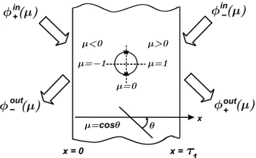
This decomposition is consistent with the half range two point boundary value prescribed in the slab problem and also with the outflux measurement, see Figure (1).
Figure 1 – One-dimensional participant medium model.
φ+(τ1)=φout,τ1 (20) If we denoteW the diagonal matrix composed with the quadrature weights,
equations (2) and (10) can be written as
Tdφ
d x = −AWφ (21)
where we are using the fact thatAis symmetric and commutes withW.
The matrix form of the direct problem is: To find
φi ∈ H1(0, τ1),i =1, . . . , M; such that equations (21), (17) and (18) hold.
In order to solve this problem we determine the discrete spectra of the matrix
T−1AW and use the spectral representation of the semi group solution,
equa-tion (15), to propagate the two point boundary values throughout the other slab points.
Note that here we have to partition the matrices in order to be consistent with the fact that we only know half range of the angular variable in each boundary position 0 andτ1.
Since we are dealing with exponential functions, for very large M will be
necessary to filter the smaller values that appear when operator A−1T is being
calculated. The numerical implementation and test cases results are presented in the next section.
In this simplified situation we can derive an explicit formula for the albedo operator,3. For this we use the exponential formula (15) and the factorization equation (14) to deduce an explicit expression for the transmission problem.
Let {φi(x),i = 1, . . . , M;0 < x ≤ τ1} a set of M linearly independent solutions. Then
8=
| | |
φ1 φ2 ∙ ∙ ∙ φM
| | |
(22)
satisfy
8(x)= Fexp(−x1)F−18(0); 0≤x ≤τ1 (23) were1is a diagonal matrix containing the eigenvalues of[T−1A].
We now adopt the two range decomposition
8= | | |
φ1− φ2− ∙ ∙ ∙ φ−M
| | |
− − − − −− − − − − −− − − − − − − − −−
| | |
φ1+ φ2+ ∙ ∙ ∙ φ+M
| | | (24)
decompose the matrix 8(x) in four parts, 8mm(x), 8mp(x), 8pm(x) and
8pp(x)as shown
8(x)= | | |
φmm(x) | φmp(x)
| | |
− − − − −− − − − − − − − −−
| | |
φpm(x) | φpp(x)
| | | (25)
following way
8(0)= | | |
φmm(0) | φmp(0)
| | |
− − − − −− − − − − − − − −−
| | |
I | 0
| | | (26) and
8(τ1)= | | |
0 | I
| | |
− − − − −− − − − − − − − −−
| | |
φpm(τ1) | φpp(τ1)
| | | (27)
where φpm(0) = I and φmp(τ1) = I are the prescribed intensities for the external sources, φpp(0) = 0 and φmm(τ1) = 0 are the respective boundary conditions of zero flux in the other side of the domain; and φmm(0), φmp(0),
φpm(τ1), and φpp(τ1) are the unknown emergent fluxes (or radiation intensi-ties) to be calculated with the albedo operator, or if this is not directly known, measured experimentally.
The transmission operator is
T r(x,x0)=U(x−x0)=exp[−(x−x0)T−1A] (28) Introducing Eqs. (25) and (26) into Eq. (15) we write
0 | I
− − −− | − − −− φpm(τ1) | φpp(τ1)
=T r
φmm(0) | φmp(0)
− − −− | − − −−
I | 0
(29)
where T r can also be partitioned in combinations of the two ranges as
T r =
T rmm | T rmp
− − −− | − − −−
T rpm | T rpp
(30)
Using the definition of the albedo operator one obtains
φmm(0) | φmp(0)
− − −− | − − −− φpm(τ1) | φpp(τ1)
=3
0 | I
− − − | − − −
I | 0
where
3=
3mm | 3mp
− − −− | − − −− 3pm | 3pp
(32)
The explicit formula of the albedo that maps the half range influx in the posi-tions{0, τ1} to the half range outflux in the same positions is then derived.
3=
T r−mm1 | −T r−mm1T rmp
− − − − − − − − − − −− | − − − − − − − − − − −−
T rpmT r−mm1 | T rpp−T rpmT r−mm1T rmp
(33)
As we have previously derived, the albedo operator establishes an explicit relation between the influx and the outflux in both sides of the slab. Since in the inverse problem we cannot suppose to know the parameters in the transmis-sion operator used to compose the albedo, we assume the knowledge of some information about its graph. In the ideal case we can suppose that we know com-pletely the albedo’s graph. In a real situation, otherwise, we can only suppose we know a linearly independent set of solutions8to the problem, derived from some finite set of experiments.
When we have M experiments to generate the columns of the matrix flux in
the two sidesx =0 andx =τ1of the slab, that is, to form the matrix equation 8(τ1)=exp−τ1T−1A8(0)
we obtain the explicit formula for A
A= −Tlog8(τ1)8−1(0)/τ1 (34) and inside A we find information about the absorption and the scattering
co-efficients. Note the resemblance that this equation has with the equation of transmission tomography [8].
In the case of multilayered slab, with transparent contiguous interfaces at positions x = τ1 < τ2 < ∙ ∙ ∙ < τN−1 and boundary surfaces at x = 0 and
x =τN, we have
8(τn)=exp
−τn−1T−1A8(τn−1); n =1, ∙ ∙ ∙, N
and
8(τN)8−1(0)=exp
" −T−1
N
X
n=1 τnAn
#
If inside each layer the operator function x 7→ A(x) is continuous in the uniform operator topology and the families {An(x),x ∈ [τn−1, τn]} are stable
[9], the formalism for integrals in the measure forx will be preserved,
8(τN)8−1(τ0)=exp
−T−1
Z τN
0
A(x)d x
(36)
The quantity inside the integral is the matrix optical thickness of the slab, and the logarithmic expression
Z τN
0
A(x)d x = −T log8(τN)8−1(0)
/τ1 (37)
is finally obtained.
The question here is about how much information can be extracted from the knowledge of the finite dimensional approximation of the albedo, and conse-quently in the operator A. Note that in general the number of parameters inAis
less than M(M+1)/2, and since in the slab problem the scattering kernel has the symmetryσs(x, ω′∙ω)=σs(x,cos(θ−θ′))which presents a convolutional
property, the maximum number in the discrete ordinates method of orderMwill
beL+1, whereL is the number of Legendre polynomials in the kernel expan-sion. Obviously,M> L+1 and we have an excess of M(M+1)/2−(L+1) degrees of freedom in the data matrix−log[8(τn)8−1(0)].
Apart from the sensitivity of the data on the coefficients, we expect to have information to treat a number of layers at least equal the integer quotient of (M(M+1)/(2(L+1)))−1. Moreover, noise and the extension of data files will probably reduce even more the number of layers that can be estimated.
Also we note that the unitary transformationFis dependent on the magnitude
of the scattering and absorption coefficients, and will highly increase the com-putational cost of non homogeneous problems. Finally, equation (34) is also appropriated for the transient problem but this question will not be discussed in this work.
5 Numerical results
In order to establish a very simple reconstruction model we note that by using the Fourier-Legendre series for the Dirichlet kernel approximation in the first part of the operatorAwe obtain
[A8](μ,x)∼=
L
X
l=0
(σt(x)−σsl(x))pl(μ)
Z +1
−1
pl(μ′)φ(ω′,x)d x
which is good for a sufficient largeL.
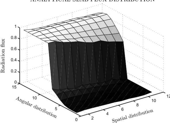
In Figure 2 we show a solution for the direct problem with M =14 discrete ordinate points.
2 4
6 8
10 12
0 5
10 15
0 0.2 0.4 0.6 0.8 1
Spatial di
stribution
ANALYTICAL SLAB FLUX DISTRIBUTION
Angular d istrib
ution
R
a
d
ia
ti
o
n
fl
u
x
Figure 2 – Typical radiation flux distribution inside a slab illuminated in one of its boundaries.
The slab is illuminated in its sidex =τ1for all ordinates. The values used for properties of this media were:σt =.5; σsl = [.4, .3, .2, .1, .0]; andτ1=1/2.
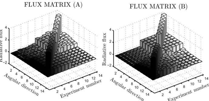
Next we present the results obtained for a inverse problem considering a set ofM =14 experiments and a slab with properties σt =.5; σsl = [.4, .3, .2,
.05, .01, .00]; and τ1 = 1/2. Figure 3 presents the fluxes matrices whose columns are the incident flux and the emergent flux in each one of M
2 4 6 8 10 12 14 2 4 6 8 10 12 14 −2 0 2 4 Experim entnum ber FLUX MATRIX (A)
Ang ular dire ction R a d ia ti v e fl u x 2 4 6 8 10 12 14 2 4 6 8 10 12 14 −2 0 2 4 Experim entnum ber FLUX MATRIX (B)
Angula r directi
on R a d ia ti v e fl u x
Figure 3 – Flux matrix at the slab boundaries.
In order to minimize the occurrence of negative fluxes we use a flux of uni-form intensity as basis for each incident flux, i.e. the incident flux total has values non negative in all directions, but with a higher value in only one direction.
Figure 4 presents the eigenvalues of these fourteen problems, the exact and the reconstructed values, respectively, for various gaussian noise levels controlled by the variance. We note the good agreement between the exact and the con-structed values when the noise level is small.
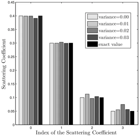
Figure 5 shows the reconstructed scattering coefficients for several gaussian noise levels and we easily deduce from the results the high sensitivity of the problem with this kind of noise, mainly for the higher order coefficients which has already been reported by Silva Neto and Özisik [11] using an implicit for-mulation for the inverse problem.
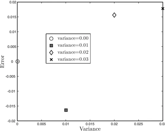
In Figure 6 we show the error in the reconstructed extinction coefficients.
6 Conclusions
In the present work and in the accompanying paper [2] we derive and show the feasibility of a new explicit formulation for the inverse radiative transfer problem. From the knowledge of the imposed incident and measured emergent radiation intensities in a one dimensional homogeneous slab we were able to estimate the anisotropic scattering coefficients, using only external detectors.
Figure 4 – Reconstructed eigenvalues for different levels of gaussian noise.
Figure 6 – Errors in the extinction coefficients reconstruction for different levels of gaussian noise.
We propose the application of this development for multilayer media and also the possibility of its use in the solution of the inverse problem of radiative trans-fer in the transient state.
Acknowledgements. The authors acknowledge the financial support pro-vided by CNPq, Conselho Nacional de Desenvolvimento Científico e Tecno-lógico, and FAPERJ, Fundação Carlos Chagas Filho de Amparo à Pesquisa do Estado do Rio de Janeiro.
REFERENCES
[1] Ch. Abrahamsson, T. Svensson, S. Svanger and S. Andersson-Engels,Time and wavelength resolved spectroscopy of turbid media using light continuum generated in a crystal fiber. Opt. Express,12(17) (2004), 4102–4112.
[2] N.I. Alvarez Acevedo, N.C. Roberty and A.J. Silva Neto, An explicit formulation for the inverse transport problem using only external detectors. Part I: Computational Modelling.
Computational & Applied Mathematics (2010).
[4] M.-J. Jeong and N.C. Hsu,Retrieval of aerosol single-scattering albedo and effective aerosol layer height for biomass-burning smoke: Sinergy derived from “A-Train” sensors. Geophys. Res. Lett.,35(2008), L24801, doi:10.1029/2008GLL036279.
[5] H.G. Kaper, C.G. Lekkerkjer and J. Hejtmanek,Spectral methods in linear transport theory. Operator theory: Advances and applications, Birkhäuser, Verlag, Basel, 5 (1982).
[6] T. Kato,Perturbation theory of linear operators. Classics in Mathematics, Springer-Verlag,
Berlin (1995).
[7] M. Koseki, Sh. Hashimoto, Sh. Sato and H. Kimura,CT Image reconstruction algorithm to reduce metal artifact. Journal of Solid Mechanics and Materials Engineering, online ISSN: 1880-9871,2(3) (2008), 374–383.
[8] F. Natterer, Algorithms in tomography. The State of Art in Numerical Analysis, Clarendon
Press, New York,63(1997).
[9] A. Pazy, Semigroups of linear operators and applications to partial differential equations. Applied Mathematical Science, Springer-Verlag, New York,44(1983).
[10] A.J. Silva Neto,Explicit and implicit formulations for inverse radiative transfer problems. 5th. World Congress on Computational Mechanics, Mini-Symposium MS125-Computational Treatment of Inverse Problems in Mechanics, Vienna, Austria (2002).
[11] A.J. Silva Neto and M.N. Özisik, An inverse problem of simultaneous estimation of radi-ation phase function, albedo and optical thickness. J. Quant. Spectrosc. Radiat. Transfer,
53(4) (1995), 397–409.
[12] K. Stamnes, H. Eide, W. Li, R. Spurr and J.J. Stamnes, Simultaneous retriefal of aerosols and marine constituents in coastal waters. Gayana online ISSN 0717-6538: Pan Ocean Remote Sensing Conference 2004, Concepción, Chile. Proc., Univ. de Concepción, Chile,