ISSN 0101-8205 www.scielo.br/cam
Using truncated conjugate gradient method
in trust-region method with two subproblems
and backtracking line search
∗MINGYUN TANG1 and YA-XIANG YUAN2
1College of Science, China Agricultural University, Beijing, 100083, China 2State Key Laboratory of Scientific Engineering Computing, Institute of Computational
Mathematics and Scientific/Engineering Computing, Academy of Mathematics and Systems Science, Chinese Academy of Sciences, P.O. Box 2719, Beijing, 100190, China
E-mails: [email protected] / [email protected]
Abstract. A trust-region method with two subproblems and backtracking line search for solving unconstrained optimization is proposed. At every iteration, we use the truncated conjugate gradient method or its variation to solve one of the two subproblems approximately. Backtracking line search is carried out when the trust-region trail step fails. We show that this method have the same convergence properties as the traditional trust-region method based on the truncated conjugate gradient method. Numerical results show that this method is as reliable as the traditional one and more efficient in respect of iterations, CPU time and evaluations.
Mathematical subject classification: Primary: 65K05; Secondary: 90C30.
Key words: truncated conjugate gradient, trust-region, two subproblems, backtracking, con-vergence.
1 Introduction
Consider the unconstrained optimization problem
min
x∈Rn f(x), (1)
#CAM-99/09. Received: 28/IV/09. Accepted: 30/VI/09.
where f is a real-valued twice continuously differentiable function, which we assume bounded below. Unconstrained optimization problems are essential in mathematical programming because they occur frequently in many real-world applications and the methods for such problems are fundamental in the sense that these methods can be either directly applied or extended to optimization problems with constraints. There are many effective algorithms designed for unconstrained optimization problems (see [6, 13]), most of the algorithms can be classified into two categories: line search algorithm and trust region algorithms. Trust-region method is efficient for solving (1). It has mature framework, strong convergence properties and satisfactory numerical results (see [4]). How-ever, sometimes the trust-region step may be too conservative, especially when the objective function has large “convex basins”. The standard trust-region tech-nique may require quit a few iterations to stretch the trust region in order to contain the local minimizer. Thus, it is natural for us to consider modifying the standard trust region method to give an new algorithm which can maintain the convergence properties of the standard trust-region method and need less computational cost.
In the previous research [12], we obtained a trust-region method with two subproblems and backtracking line search. A subproblem without trust-region constraint was introduced into the trust-region framework in order to use the unit stepsize Newton step. This unconstrained subproblem normally gives a longer trail step, consequently it is likely that the overall algorithm will reduce the computational cost. Based on the information in the previous iterations, either the trust-region step or the Newton step is used. Moreover, the idea of combining trust-region and line search techniques (see [8]) is also used in that algorithm. The algorithm inherits the convergence result of traditional trust-region method and gives better performance by making good use of the Newton step and backtracking line search. However, as the exact minimizer of the trust-region subproblem is need and the Cholesky factorization of the Hessian matrix is used to decide whether the model function is convex, that algorithm is obvi-ously not fit for large problems.
solve the subproblems. Our method can be regarded as a modification to the standard trust region method for unconstrained optimization in such a way that the Newton step can be taken as often as possible. A slightly modified trun-cated conjugate gradient method is used to compute the Newton step. The global convergence and local superlinear convergence results of the algorithm are also given in the paper.
The paper is organized as follows. In the next section, we give the framework of the method and describe our new algorithm. The convergence properties are presented in Section 3 and the numerical results are provided in Section 4. Some conclusions are given in Section 5.
2 The algorithm
First we briefly review the framework of trust-region method with two subprob-lems and backtracking line search.
One of the two subproblems is the trust-region subproblem. At the current iterationxk, the trust-region subproblem is
( min
s∈Rn Qk(s)=g T ks+
1 2s
TH ks,
s.t. ksk ≤1k
, (1)
whereQk(s)is the approximate model function of f(x)within the trust-region,
gk = g(xk) = ∇f(xk) and Hk = ∇2f(xk)or an approximation of ∇2f(xk).
We usually chooseQk to be the first three terms of the Taylor expansion of the
objective function f(x)atxkwith the constant term f(xk)being omitted as this
term does not influence the iteration process. Another subproblem is defined by
min
s∈RnQk(s)=g T ks+
1 2s
TH
ks, (2)
wheregk,Hk has the same meaning as in (2). Since in this subproblem we do
not require the trust region constraint, we call it unconstrained subproblem. In the ideal situation, the unconstrained subproblem should be used when the model function is convex and gives an accurate approximation to the objective function. Define
ρk =
f(xk)− f(xk+s)
Qk(0)−Qk(s)
The ratioρk is used by trust region algorithms to decide whether the trial step
is acceptable and how to update the trust-region radius. In the method given in [12], we also use the value of ρk and the positive definiteness of ∇2f(xk)
to decide the model choice since we solve the trust-region subproblem exactly. In this paper, we use the truncated conjugate gradient method (see [1, 10]) to compute a minimizer of the trust-region subproblem approximately, as Cholesky factorization cannot be used for large scale problems. Now, we consider how to compute the unconstrained model minimizer approximately.
Consider using the conjugate gradient method to solve the subproblem (3). The subscriptidenotes the interior iteration number. If we do not know whether our quadratic model is strictly convex, precautions must be taken to deal with non-convexity if it arises. Similarly to the analysis of the truncated conjugate gradient method (see [4]), if we minimize Qk without considering whether or
not∇2f(x
k)is positive definite, the following two possibilities might arise:
(i) the curvaturehpi,H piiis positive at each iteration. This means the current
model function is convex along direction pi, as we expect. In this case,
we just need to continue the iteration of the conjugate gradient method.
(ii) hpi,H pii ≤ 0. This means the model function is not strictly convex.
Qk is unbounded from below along the linesi +σpi. The unconstrained
subproblem is obviously not fit for reflecting the condition of the objective function around the current iteration now. So we should add the trust-region constraint and minimize Qk along si +σpi as much as we can
while staying within the trust region. In this case, what we need to do is finding the positive root ofksi +σpik =1.
In order to avoid conjugate gradient iterations that make very little progress in the reduction of the model quadratical function, the iteration are also terminated if one of the following conditions
k∇Qk(sj)k ≤10−2k∇Qk(0)k, (4)
Qk(sj−1)−Qk(sj)
≤10−2
Qk(0)−Qk(sj)
(5)
Now, we can give an algorithm for solving the unconstrained subproblem approximately. It is a variation of the truncated conjugate gradient method.
Algorithm 2.1
Step 1 Initialization Set s0 =0,v0 =g0= ∇xf(xk), p0 = −g0, cur q =0,
pr eq =1, kappag=0.01,εk =min(kappag,√kg0k), i ter max =
n.
Step 2 While i≤ i ter max
if pr eq−cur q ≤kappag∗(−cur q), stop.
κi = piTH pi,
ifκi ≤0, then
info:=1, ifksik ≥1kthen stop, else computeσ as the
positive root ofksi+σpik =1k, si+1=si +σpi, stop.
end if
αi = hgi, vii/κi,
si+1=si +αipi,
update pr eq, cur q, gi+1,
ifkgi+1k/kg0k ≤εk, stop.
vi+1=gi+1,
βi = hgi+1, vi+1i/hgi, vii,
pi+1= −vi+1+βipi,
i =i+1,
goto step 2.
above algorithm is faster than solvingHks = −gkby carrying out the Cholesky
factorization ofHkdirectly.
We now describe the algorithm of using truncated conjugate gradient method in the trust-region method with two subproblems and backtracking line search. We useρk and flaginfo to decide the model choice. If the value of ρk of an
unconstrained subproblem is smaller than a positive constantη2ori n f o = 1,
we may consider that the unconstrained model is not proper and choose the trust-region subproblem in the next iteration. We take the unconstrained model if the ratioρk of the trust-region trail step is bigger than a constant β (β → 1 and
β <1) in 2 consecutive steps. The overall algorithm is given as follows.
Algorithm 2.2 (A trust region method with two subproblems)
Step 1 Initialization.
An initial point x0and an initial trust-region radius10>0are given.
The stopping toleranceε is given. The constantsη1,η2,γ1,γ2andβ
are also given and satisfy0< η1≤η2< β <1and0< γ1<1≤γ2.
Set k := 0, btime:= 0 and fmi n := f(x0). Set flag T R0 := 0, info :=0.
Step 2 Determine a trial step.
if T Rk =0, then compute sk by Algorithm 2.1;
else use truncated CG method to obtain sk.
xt :=xk+sk.
Step 3 Backtracking line search.
ft := f(xt).
if ft < fmi ngo to step 4;
else if T Rk =1, then carry out backtracking line search;
else then
T Rk+1:=1,btime:=0, k :=k+1, go to step 2.
Step 4 Acceptance of the trial point and update the flag TRk+1and the
xk+1:=xt. fmi n:= f(xt).
Computeρkaccording to(4).
Update1k+1:
1k+1=
γ11k i f T Rk =1 and ρk < η1,
or T Rk =0andρk < η1 and kskk ≤1k;
γ21k i f T Rk =1 and ρk ≥η2,
or T Rk =0andρk ≥η2 and i n f o=1;
1k ot herwi se.
Update btime and T Rk+1:
bti me=
0 i f T Rk =1 and ρk ≤β ,
or T Rk =0 and ρk ≥η2 and
i n f o=1,
or T Rk =0 and 0< ρk < η2;
bti me+1 i f T Rk =1 and ρk > β.
T Rk+1=
0 i f bti me=2;
1 i f T Rk =0 and ρk ≥η2 and i n f o=1,
or T Rk =0 and 0< ρk < η2;
T Rk ot herwi se.
if btime=2, btime:=0. k :=k+1.
go to step 2.
In the above algorithm, backtracking line search is carried out using the same formula as in [12]. We try to find the minimum positive integer i such that
f(xk+αis) < f(xk),whereα ∈(0,1)is a positive constant (see [8]). The step
sizeαis computed by polynomial interpolation since f(xk),g(xk),∇2f(xk)and
f(xk +s)are all known. Denoteq = 21sT∇2f(xk)s, then
α= − g
T ks
q+
q
(q2−3gT
ks(f(xk+s)−q−gkTs− f(xk))
(6)
chooseα = −gkTs/sT∇2f(xk)s or the result of truncated quadratic
interpola-tion when the denominator equals to zero
αkis too small. It is obvious that to evaluate the objective function on two close
points is a waste of computational cost and available information. The idea of discarding small steps computed as minimizers of interpolation functions was also explored in [2] and [3].
3 Convergence
In this section we present the convergence properties of the algorithm given in the previous section.
In our algorithm, if the unconstrained subproblem is chosen and the Hessian matrix is not positive definite, the trial step will be truncated on the boundary of trust-region just the same as truncated conjugate gradient method. So the difference arises when the model function is convex and the trail step is large, which provides more decrease of the model function. Thus in fact the uncon-strained model is used only when the model function is convex. The proof of our following theorem is similar to that of Theorem 3.2 of Steihaug [11] and Powell [10].
Theorem 3.1. Suppose that f in (1)is twice continuously differentiable and bounded below and the norm of Hessian matrix is bounded. Letεkbe the relative
error in the truncated conjugate gradient method and the Algorithm 2.1. Iteration
{xk}is generated by the Algorithm 2.2. Ifεk≤ε <1, then
lim inf
k→∞ kg(xk)k =0. (1)
Proof. Since we have
Qk(sk)≤min
Qk(−σg(xk)): kσg(xk)k ≤ kskk (2)
no matter the trail step sk is computed by the trust-region subproblem or the
unconstrained subproblem, it follows from Powell’s result [10] that
−Qk(sk)≥c1kg(xk)kmin
kskk,k
g(xk)k kHkk
, (3)
withc1=
We prove the theorem by contradiction. If the theorem were not true, we can assume that
kg(xk)k ≥δfor all k. (4)
Thus, due to (4) and the boundedness ofkHkk, there exists a positive constantδ
such that
−Qk(sk)≥δmin
kskk,1 . (5)
First we show that
X
k≥0
kskk<+∞. (6)
Define the following two sets of indices:
S=k :ρk ≥η1 , (7)
U =k :T Rk =0 . (8)
Since f is bounded below, we have
+∞ > f0−min f(x)≥ ∞
X
k=1
f(xk)− f(xk+1)
(9)
≥ X k∈S
f(xk)− f(xk+1)
≥η1
X
k∈S
−Q(sk)
≥ η1δ
X
k∈S
minkskk,1 ,
which shows that
X
k∈S
kskk<+∞. (10)
Hence there existsk0such that
kskk ≥1k ∀k ≥k0, k ∈ S (11)
becausekHksk+gkk ≥ 12δfor all sufficiently largek. This shows that
First we consider the case thatU is a finite set. In this case, there exists an integerk1such thatT Rk =1 for allk≥k1and Algorithm 2.2 is essentially the
standard trust-region algorithm for all largek. Thus
1k+1≤γ11k ∀k ≥k1, k ∈/ S. (13)
Letk2=max{k0,k1}, we have that
X
k≥k2
kskk ≤
X
k≥k2,k∈S
kskk +
X
k≥k2,k∈/S
1k (14)
≤ X k≥k2,k∈S
kskk +
1k2 +γ2
P
k≥k2,k∈S1k
1−γ1
≤ 1k2
1−γ1 +
1+ γ2
1−γ1
X
k≥k2,k∈S
kskk
< +∞,
which shows that (6) is true.
Now we consider the case thatU has infinitely many elements.
Ifk ∈/ S,T Rk =0 andk is sufficiently large, we have thatT Rk+1=1 and
1k+1=
(
γ11k if kskk ≤1k,
1k if kskk> 1k.
(15)
whilek ∈/ S, T Rk = 1, always have1k+1 =γ11k. Therefore there existsk3
such that
X
k≥k3,k∈/S 1k ≤
1k3 +
X
k≥k3,k∈S 1k
2γ2
1−γ1
(16)
≤
1k3 +
X
k≥k3,k∈S
kskk
2γ2
1−γ1
.
Hence
X
k≥k3,k∈/S
Relation (10), (11) and (17) indicate that
∞
X
k=1
1k <+∞, (18)
which implies that limk→∞1k =0. Therefore, whenk → +∞andkskk ≤1k,
we have
ρk →1. (19)
Thus,1k+1≥ 1k ifk is sufficiently large and ifkskk ≤1k. Ifkskk> 1k, we
know thatT Rk = 0, our algorithm gives either1k+1 = 1k or1k+1 = γ21k.
This shows that1k+1≥1kfor all largek. This contradicts to (18). So (4) must
therefore be false, which yields (1).
The above theorem shows that our algorithm is globally convergent. Fur-thermore, we can show that our algorithm converges superlinearly if certain conditions are satisfied.
Theorem 3.2. Suppose that f in(1)in Section 1 is twice continuously differ-entiable and bounded below and the norm of Hessian matrix is bounded, the iteration{xk}generated by Algorithm 2.2 satisfies xk →x∗as k → ∞and the
Hessian matrix H(x∗)of f is positive definite. Letε
kbe the relative error in the
truncated conjugate gradient method and Algorithm 2.1. If εk → 0then {xk}
converges superlinearly, i.e.,
lim
k→∞
kxk+1−x∗k kxk−x∗k =
0. (20)
Proof. Because xk → x∗ and H(x∗) > 0, there exists k1 such that kH−1(x
k)k ≤ 2kH−1(x∗)kfor all k ≥ k1. Therefore the Newton step skN = −H−1(x
k)g(xk)satisfies that
kskNk ≤2kH−1(x∗)kkg(xk)k (21)
for allk ≥ k1. Therefore, no mattersk generated by our algorithm is a
trust-region step or a truncated Newton step, we have that
Our previous theorem implies thatkg(xk)k →0. Inequality (22) shows that
lim
k→∞ρk =1. (23)
Consequently, xk+1 = xk +sk and 1k+1 ≥ 1k for all sufficiently large k.
Consequently,kskk < 1k for all sufficiently large k. Namelysk is an inexact
Newton step for all largek, which indicates that
kg(xk)+Hkskk/kg(xk)k ≤εk, (24)
for all sufficiently largek. Relation (24) shows that
lim
k→∞
kg(xk+1)k kg(xk)k =
lim
k→∞
kg(xk+sk)k kg(xk)k
(25)
= lim
k→∞
kg(xk)+Hkskk +o(kskk) kg(xk)k
= lim
k→∞
kg(xk)+Hkskk kg(xk)k ≤ lim
k→∞εk =0.
Now, (20) follows from the fact that H(x∗) >0 andxk →x∗.
4 Numerical results
In this section we report numerical results of our algorithm given in Section 2, and we also compare our algorithm with traditional trust region algorithm as given in [6, 13]. Test problems are the 153 unconstrained problems from the CUTEr collection (see [7]). The names and dimensions of the problems are given in Tables 1-3.
Problem n Problem n Problem n
AKIVA 2 CURLY10 1000 DJTL 2
ALLINITU 4 CURLY20 1000 DQDRTIC 1000 ARGLINA 100 CURLY30 1000 DQRTIC 1000 ARGLINB 100 DECONVU 61 EDENSCH 2000
ARGLINC 10 DENSCHNA 2 EG2 1000
ARWHEAD 1000 DENSCHNB 2 EIGENALS 110 BARD 3 DENSCHNC 2 EIGENBLS 110 BDQRTIC 1000 DENSCHND 2 EIGENCLS 30
BEALE 2 DENSCHNE 2 ENGVAL1 1000
BIGGS6 6 DENSCHNF 2 ENGVAL2 3
BOX3 3 DIXMAANA 1500 ERRINROS 50 BRKMCC 2 DIXMAANB 1500 EXPFIT 2 BROWNAL 10 DIXMAANC 300 EXTROSNB 10
Table 1 – Test problems and corresponding dimensions.
parameters are not sensitive to the algorithm. So we choose the common values as (for example, see [6, 13])γ1=0.25, γ2 =2,η1 =0.1,η2=0.75,β =0.9,
10=1.The truncated conjugate gradient method (see [11]) is used to solve the
trust-region subproblem. Both algorithms stop ifk∇f(xk)k ≤10−6.
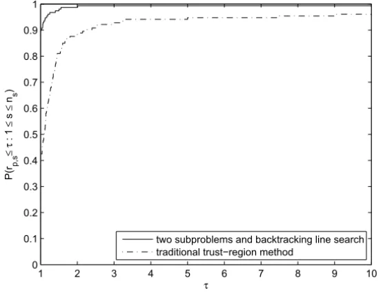
Our algorithm solved 125 problems out of the 153 CUTEr test problems, while the traditional trust-region method solved 120 problems. Failure often occurs because the maximal iteration number is reached. Thus, we found that the new algorithm is as reliable as the traditional one.
Problem n Problem n Problem n BROWNBS 2 DIXMAAND 300 FLETCBV2 1000 BROWNDEN 4 DIXMAANE 300 FLETCBV3 10
BROYDN7D 1000 DIXMAANF 300 FLETCHBV 10 BRYBND 1000 DIXMAANG 300 FLETCHCR 100 CHAINWOO 1000 DIXMAANH 300 FMINSRF2 121 CHNROSNB 50 DIXMAANI 300 FMINSURF 121 CLIFF 2 DIXMAANJ 300 FREUROTH 500 COSINE 10 DIXMAANK 15 GENHUMPS 500 CRAGGLVY 100 DIXMAANL 300 GENROSE 100 CUBE 2 DIXON3DQ 1000 GROWTHLS 3 GULF 3 MAQRTBLS 100 SCOSINE 10 HAIRY 2 NONCVXU2 100 SCURLY10 100 HATFLDD 3 NONCVXUN 100 SCURLY20 100 HATFLDE 3 NONDIA 1000 SCURLY30 100 HEART6LS 6 NONDQUAR 1000 SENSORS 10 HEART8LS 8 NONMSQRT 49 SINEVAL 2
HELIX 3 OSBORNEA 5 SINQUAD 500
HIELOW 3 OSBORNEB 11 SISSER 2
HILBERTA 2 OSCIPATH 15 SNAIL 2
HILBERTB 10 PALMER1C 8 SPARSINE 1000 HIMMELBB 2 PALMER1D 7 SPARSQUR 1000 HIMMELBF 4 PALMER2C 8 SPMSRTLS 499 HIMMELBG 2 PALMER3C 8 SROSENBR 1000 HIMMELBH 2 PALMER4C 8 STRATEC 10
HUMPS 2 PALMER5C 6 TESTQUAD 1000 HYDC20LS 99 PALMER6C 8 TOINTGOR 50
INDEF 1000 PALMER7C 8 TOINTGSS 1000 JENSMP 2 PALMER8C 8 TOINTPSP 50 KOWOSB 4 PENALTY1 100 TIONTQOR 50 LIARWHD 1000 PENALTY2 100 TQUARTIC 1000
Problem n Problem n Problem n LOGHAIRY 2 PENALTY3 50 TRIDIA 1000
MANCINO 100 POWELLSG 1000 VARDIM 100 MARATOSB 2 POWER 100 VAREIGVL 50
MEXHAT 2 QUARTC 1000 VIBRBEAM 8
MEYER3 3 ROSENBR 2 WATSON 12
MODBEALE 2000 S308 2 WOODS 1000
MOREBV 1000 SBRYBND 100 YFITU 3 MSQRTALS 100 SCHMVETT 1000 ZANGWIL2 2
Table 3 – Test problems and corresponding dimensions.
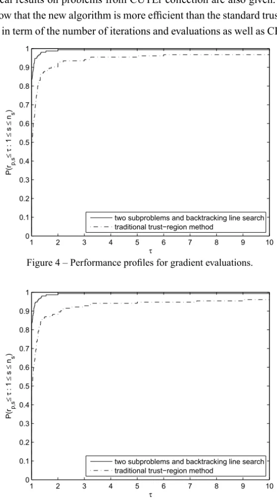
algorithm is also shown by total number of evaluations since it is dominative on 77 problems.
It is easy to see from these figures that the new algorithm is more efficient than the traditional trust-region algorithm.
1 2 3 4 5 6 7 8 9 10
0 0.1 0.2 0.3 0.4 0.5 0.6 0.7 0.8 0.9 1
τ
P
(rp
,s
≤
τ
:
1
≤
s
≤
ns
)
two subproblems and backtracking line search traditional trust−region method
Figure 1 – Performance profiles for iterations.
5 Conclusions
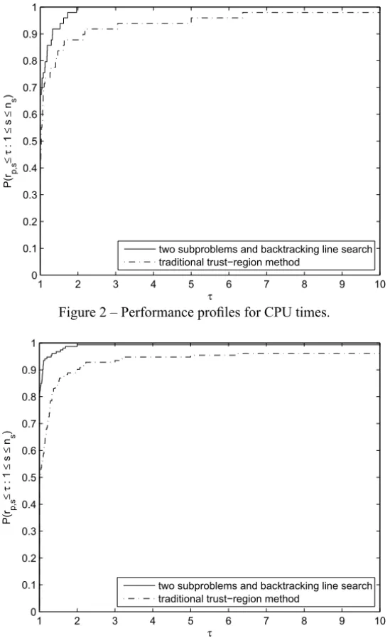
1 2 3 4 5 6 7 8 9 10 0
0.1 0.2 0.3 0.4 0.5 0.6 0.7 0.8 0.9 1
τ
P
(r p
,s
≤
τ
:
1
≤
s
≤
n s
)
two subproblems and backtracking line search traditional trust−region method
Figure 2 – Performance profiles for CPU times.
1 2 3 4 5 6 7 8 9 10
0 0.1 0.2 0.3 0.4 0.5 0.6 0.7 0.8 0.9 1
τ
P
(r p
,s
≤
τ
:
1
≤
s
≤
n s
)
two subproblems and backtracking line search traditional trust−region method
Figure 3 – Performance profiles for function evaluations.
Numerical results on problems from CUTEr collection are also given. The re-sults show that the new algorithm is more efficient than the standard trust-region method in term of the number of iterations and evaluations as well as CPU time.
1 2 3 4 5 6 7 8 9 10
0 0.1 0.2 0.3 0.4 0.5 0.6 0.7 0.8 0.9 1
τ
P
(r p
,s
≤
τ
:
1
≤
s
≤
n s
)
two subproblems and backtracking line search traditional trust−region method
Figure 4 – Performance profiles for gradient evaluations.
1 2 3 4 5 6 7 8 9 10
0 0.1 0.2 0.3 0.4 0.5 0.6 0.7 0.8 0.9 1
τ
P
(r p
,s
≤
τ
:
1
≤
s
≤
n s
)
two subproblems and backtracking line search traditional trust−region method
Acknowledgements. The authors would like to thank an anonymous referee for his valuable comments on an earlier version of the paper.
REFERENCES
[1] E.G. Birgin and J.M. Martínez,Large-scale active-set box-constrained optimization method with spectral projected gradients.Computational Optimization and Applications,23(2002), 101–125.
[2] E.G. Birgin, J.M. Martínez and M. Raydan,Nonmonotone spectral projected gradient methods on convex sets.SIAM Journal on Optimization,10(2000), 1196–1211.
[3] E.G. Birgin, J.M. Martínez and M. Raydan, Algorithm 813: SPG – software for convex-constrained optimization. ACM Transactions on Mathematical Software,27(2001), 340– 349.
[4] A.R. Conn, N.I.M. Gould and Ph.L. Toint, Trust-Region Methods. SIAM, Philadelphia, USA, (2000).
[5] E.D. Dolan and J.J. Moré, Benchmarking optimization software with performance profiles.
Mathematical Programming,91(2) (2002), 201–213.
[6] R. Fletcher, Practical Methods of Optimization, Vol. 1, Unconstrained Optimization. John Wiley and Sons, Chichester, (1980).
[7] N.I.M. Gould, D. Orban and Ph.L. Toint, CUTEr (and SifDec), a constrained and uncon-strained testing environment, revisited. Transactions of the ACM on Mathematical Software,
29(4) (2003), 373–394.
[8] J. Nocedal and Y. Yuan, Combining trust region and line search techniques. Advances in Nonlinear Programming, (1998), 153–175.
[9] M.J.D. Powell,The NEWUOA software for unconstrained optimization without derivatives.
Large-Scale Nonlinear Optimization,83(2006), 256–297, Springer, USA.
[10] M.J.D. Powell, Convergence properties of a class of minimization algorithms. Nonlinear Programming 2, Eds. O.L. Mangasarian, R.R. Meyer and S.M. Robinson, (1975), Academic Press, New York.
[11] T. Steihaug,The Conjugate Gradient Method and Trust Regions in Large Scale Optimization.
SIAM J. Numer. Anal.,20(3) (1983), 626–637.
[12] M.Y. Tang, A trust-region-Newton method for unconstrained optimization. Proceedings of the 9th National Conference of ORSC, Eds. Y. Yuan, X.D. Hu and D.G. Liu, (2008), Global-Link, Hong Kong.