ISSN 0101-8205 www.scielo.br/cam
Picard and Adomian methods for quadratic
integral equation
EL-SAYED A.M.A.1, HASHEM H.H.G.2 and ZIADA E.A.A.2
1Faculty of Science, Alexandria University, Alexandria, Egypt 2Faculty of Engineering, Mansoura University, Mansoura, Egypt E-mails: [email protected] / [email protected] /
Abstract. We are concerning with two analytical methods; the classical method of successive approximations (Picard method) [14] which consists the construction of a sequence of functions such that the limit of this sequence of functions in the sense of uniform convergence is the solution of a quadratic integral equation, and Adomian method which gives the solution as a series see ([1-6], [12] and [13]). The existence and uniqueness of the solution and the convergence will be discussed for each method.
Mathematical subject classification: Primary: 39B82; Secondary: 44B20, 46C05.
Key words:quadratic integral equation, Picard method, Adomian method, continuous unique solution, convergence analysis, error analysis.
1 Introduction
Quadratic integral equations (QIEs) are often applicable in the theory of radia-tive transfer, kinetic theory of gases, in the theory of neutron transport and in the traffic theory. The quadratic integral equations can be very often encountered in many applications.
The quadratic integral equations have been studied in several papers and monographs (see for examples [7-11] and [16-22]).
The Picard-Lindelof theorem for the initial value problem
x′(t)= f(t,x(t)), x(0)=x0
was proved in [14] and the solution can be shown as the limit of constructed sequence.
The existence of continuous solution of the nonlinear quadratic integral equa-tion
x(t)=a(t)+g(t,x(t)) Z t
0
f(s,x(s))ds (1)
was proved in [18] by using Tychonov fixed point theorem where f andgsatisfy Carathéodory condition.
In this work, we will prove the existence and the uniqueness of continuous solution for (1) by using the principle of contraction mapping. Also, we are concerning with the two methods; Picard method and Adomian method.
2 Main Theorem
Now, equation (1) will be investigated under the assumptions:
(i) a :I → R+ = [0,+ ∞)is continuous on I whereI = [0,1];
(ii) f, g : I ×D ⊂ R+ → R+are continuous and there exist positive con-stantsM1andM2such that|g(t,x)| ≤M1and|f(t,x)| ≤M2onD;
(iii) f,g satisfy Lipschitz condition with Lipschitz constantsL1andL2such that,
|g(t,x)−g(t,y)| ≤ L1|x −y|, |f(t,x)− f(t,y)| ≤ L2|x −y|.
LetC =C(I)be the space of all real valued functions which are continuous onI.
Define the operator Fas
(F x)(t)=a(t)+g(t,x(t)) Z t
0
Theorem 1. Let the assumptions (i)-(iii) be satisfied. If h = (L1M2 + L2M1) < 1, then the nonlinear quadratic integral equation(1) has a unique positive solution x∈C.
Proof. It is clear that the operatorF mapsC intoC.
Now define a subsetSofCas
S = {x ∈C: |x−a(t)| ≤k}, k= M1M2.
Then the operatorF mapsSinto S, since forx ∈ S
|x(t)−a(t)| ≤M1M2
Z t
0
ds =M1M2t =M1M2.
Moreover it is easy to see that Sis a closed subset ofC. In order to show that Fis a contraction we compute
(F x)(t)−(F y)(t) = g(t,x(t)) Z t
0
f(s,x(s))ds
−g(t,y(t)) Z t
0
f(s,y(s))ds+g(t,x(t))
×
Z t
0
f(s,y(s))ds −g(t,x(t)) Z t
0
f(s,y(s))ds
= [g(t,x(t))−g(t,y(t))]
Z t
0
f(s,y(s))ds
+g(t,x(t)) Z t
0
[f(s,x(s))− f(s,y(s))]ds
|(F x)(t)−(F y)(t)| ≤ |g(t,x(t))−g(t,y(t))|
Z t
0
|f(s,y(s))|ds
+|g(t,x(t))|
Z t
0
|f(s,x(s))− f(s,y(s))|ds
≤ L1M2|x −y| +L2M1
Z t
0
|x(s)−y(s)|ds
||(F x)(t)−(F y)(t)|| = max
t∈I |(F x)(t)−(F y)(t)|
≤ L1M2||x−y|| +L2M1||x−y|| ≤ (L1M2+L2M1)||x −y||
Since
h=(L1M2+L2M1) <1,
then F is a contraction and F has a unique fixed point inS, thus there exists a
unique solution for (1).
3 Method of successive approximations (Picard method)
Applying Picard method to the quadratic integral equation (1), the solution is constructed by the sequence
xn(t) = a(t)+g(t,xn−1(t))
Z t
0
f(s,xn−1(s))ds, n =1,2, . . . ,
x0(t) = a(t). (2)
All the functionsxn(t)are continuous functions andxncan be written as a sum of successive differences:
xn=x0+ n
X
j=1
(xj −xj−1),
This means that convergence of the sequencexnis equivalent to convergence of the infinite seriesP
(xj−xj−1)and the solution will be, x(t)= lim
n→∞ xn(t), i.e. if the infinite seriesP
(xj −xj−1)converges, then the sequencexn(t)will converge tox(t). To prove the uniform convergence of{xn(t)}, we shall consider the associated series
∞
X
n=1
[xn(t)−xn−1(t)].
From (2) forn=1, we get
x1(t)−x0(t)=g(t,x0(t)) Z t
0
f(s,x0(s))ds
and
|x1(t)−x0(t)| ≤M1M2
Z t
0
Now, we shall obtain an estimate forxn(t)−xn−1(t), n ≥2
xn(t)−xn−1(t)≤g(t,xn−1(t))
Z t
0
f(s,xn−1(s))ds
−g(t,xn−2(t))
Z t
0
f(s,xn−2(s))ds+ g(t,xn−1(t))
×
Z t
0
f(s,xn−2(s))ds− g(t,xn−1(t))
Z t
0
f(s,xn−2(s))ds
≤g(t,xn−1(t))
Z t
0
[f(s,xn−1(s))− f(s,xn−2(s))]ds
+ [g(t,xn−1(t))−g(t,xn−2(t))]
Z t
0
f(s,xn−2(s))ds,
using assumptions (ii) and (iii), we get
|xn(t)−xn−1(t)| ≤M1L2
Z t
0
|xn−1(s)−xn−2(s)|ds
+M2L1|xn−1(t)−xn−2(t)|
Z t
0 ds.
Puttingn=2, then using (3) we get
|x2(t)−x1(t)| ≤ M1L2
Z t
0
|x1(s)−x0(s)|ds+M2L1|x1(t)−x0(t)|t.
|x2−x1| ≤ M12M2L2 t2
2 +M1M 2 2L1t
2
≤ M1M2
1
2M1L2+M2L1
t2
|x3−x2| ≤ M1L2
Z t
0
|x2(s)−x1(s)|ds+M2L1|x2(t)−x1(t)|
Z t
0 ds
≤ M1M2
1
2M1L2+M2L1 1
3M1L2+M2L1
t3.
Repeating this technique, we obtain the general estimate for the terms of the series:
|xn−xn−1| ≤ M1M2
1
2M1L2+M2L1 1
3M1L2+M2L1
×∙ ∙ ∙×
1
nM1L2+M2L1
≤ M1M2
1
2M1L2+M2L1 1
3M1L2+M2L1
×∙ ∙ ∙×
1
nM1L2+M2L1
≤ M1M2(M1L2+M2L1)(M1L2+M2L1)×∙ ∙ ∙×(M1L2+M2L1) ≤(M1L2+M2L1)n.
Since(L1M2+L2M1) <1, then the uniform convergence of ∞
X
n=1
xn(t)−xn−1(t)
is proved and so the sequence{xn(t)}is uniformly convergent. Since f(t,x)andg(t,x)are continuous inx, then
x(t) = lim
n→∞g(t,xn(t))
Z t
0
f(s,xn(s))ds
= g(t,x(t)) Z t
0
f(s,x(s))ds.
thus, the existence of a solution is proved.
To prove the uniqueness, lety(t)be a continuous solution of (1). Then
y(t)=a(t)+g(t,y(t)) Z t
0
f(s,y(s))ds t∈ [0,1]
and
y(t)−xn(t)≤g(t,y(t))
Z t
0
f(s,y(s))ds−g(t,xn−1(t))
Z t
0
f(s,xn−1(s))ds
+ g(t,y(t))
Z t
0
f(s,xn−1(s))ds−g(t,y(t))
Z t
0
f(s,xn−1(s))ds
=g(t,y(t))
Z t
0
[f(s,y(s))− f(s,xn−1(s))]ds + [g(t,y(t))−g(t,xn−1(t))]
Z t
0
f(s,xn−1(s))ds, using assumptions (ii) and (iii), we get
|y(t)−xn(t)| ≤ M1L2
×
Z t
0
|y(s)−xn−1(s)|ds+M2L1|y(t)−xn−1(t)|
Z t
0 ds.
But
|y(t)−a(t)| ≤M1M2t,
and using (4) then we get
|y(t)−xn(t)| ≤(M1L2+M2L1)n. Hence
lim
n→∞xn(t)= y(t)=x(t) ,
which completes the proof.
Wheng(t,x)=1, thenM1=1 andL1=0 and we obtain the original Picard theorem [14] and [15].
Corollary 1. Let the assumptions of Theorem 1 (with g(t,x) = 1) be satis-fied. If L2<1, then the integral equation
x(t)=x0(t)+
Z t
0
f(s,x(s))ds
has a unique continuous solution.
4 Adomian Decomposition Method (ADM)
The Adomian decomposition method (ADM) is a nonnumerical method for solving a wide variety of functional equations and usually gets the solution in a series form.
a large amount of applications in applied sciences. For more details about the method and its application, see ([1-6] and [12-13]).
In this section, we shall study Adomian decomposition method (ADM) for the quadratic integral equation (1).
The solution algorithm of the quadratic integral equation (1) using ADM is,
x0(t) = a(t), (5)
xi(t) = A(i−1)(t) Z t
0
B(i−1)(s)ds. (6) where Ai andBi are Adomian polynomials of the nonlinear terms g(t,x)and
f(s,x)respectively, which have the form
An = 1 n!
dn dλn
"
f t,
∞
X
i=0
λixi
!#
λ=0
, (7)
Bn = 1 n!
dn dλn
"
g t,
∞
X
i=0
λixi
!#
λ=0
(8)
and the solution will be,
x(t)= ∞
X
i=0
xi(t) (9)
4.1 Convergence analysis
Theorem 2. Let the solution of the QIE (1)exists. If|x1(t)| <l,l is a posi-tive constant, then the series solution(9)of the QIE(1)using ADM converges.
Proof. Define the sequenceSp such that,
Sp= p
X
i=0 xi(t)
is the sequence of partial sums from the series solutionP∞
i=0 xi(t), and we have g(t,x) =
∞
X
i=0 Ai,
f(s,x) = ∞
X
LetSpandSq be two arbitrary partial sums with p >q. Now, we are going to prove that
Sp is a Cauchy sequence in this Banach spaceE.
Sp−Sq = p
X
i=0 xi−
q X i=0 xi = p X i=0
A(i−1)(t) Z t
0 p
X
i=0
B(i−1)(s)ds− q
X
i=0
A(i−1)(t) Z t
0 q
X
i=0
B(i−1)(s)ds
= p
X
i=0
A(i−1)(t) Z t
0 p
X
i=0
B(i−1)(s)ds− q
X
i=0
A(i−1)(t) Z t
0 p
X
i=0
B(i−1)(s)ds
+ q
X
i=0
A(i−1)(t) Z t
0 p
X
i=0
B(i−1)(s)ds− q
X
i=0
A(i−1)(t) Z t
0 q
X
i=0
B(i−1)(s)ds
=
" p X
i=0
A(i−1)(t)− q
X
i=0
A(i−1)(t) # Z t 0 p X i=0
B(i−1)(s)ds
+ q
X
i=0
A(i−1)(t) Z t
0
" p
X
i=0
B(i−1)(s)− q
X
i=0
B(i−1)(s) #
ds
Sp−Sq ≤max
t∈I
p X
i=q+1
A(i−1)(t) Z t
0 p
X
i=0
B(i−1)(s)ds +max t∈I
q X i=0
A(i−1)(t) Z t
0 p
X
i=q+1
B(i−1)(s)ds ≤max t∈I
p−1 X
i=q Ai(t)
Z t 0 p X i=0
B(i−1)(s)ds ds +max t∈I
q X i=0
A(i−1)(t) Z t 0 p−1 X
i=q Bi(s)
ds ≤max t∈I
g(t,Sp−1)−g(t,Sq−1)
Z t
0
f(t,Sp)
ds
+max t∈I
g(t,Sq)
Z t
0
f(t,Sp−1)− f(t,Sq−1)
ds
≤ L1M2 max t∈I
Sp−1−Sq−1
+L2M1 max
t∈I
Sp−1−Sq−1
Letp =q+1 then,
Sq+1−Sq
≤h
Sq−Sq−1
≤h2
Sq−1−Sq−2
≤ ∙ ∙ ∙ ≤hqkS1−S0k
From the triangle inequality we have,
Sp−Sq ≤
Sq+1−Sq +
Sq+2−Sq+1
+ ∙ ∙ ∙ +
Sp−Sp−1
≤
hq+hq+1+ ∙ ∙ ∙ +hp−1
kS1−S0k
≤ hq1+h+ ∙ ∙ ∙ +hp−q−1kS1−S0k ≤ hq
1−hp−q 1−h
kx1(t)k
Now 0<h <1, and p >qimplies that(1−hp−q)≤1. Consequently,
Sp−Sq
≤
hq
1−h kx1(t)k
≤ h
q
1−h maxt∈I |x1(t)| but,|x1(t)|<land asq → ∞then,Sp−Sq
→0 and hence,
Sp is a Cau-chy sequence in this Banach spaceEand the series P∞
i=0xi(t) converges.
4.2 Error analysis
Theorem 3. The maximum absolute truncation error of the series solution(9)
to the problem(1)is estimated to be,
max t∈I
x(t)− q
X
i=0 xi(t)
≤ h q
1−h maxt∈I |x1(t)|
Proof. From Theorem 2 we have,
Sp−Sq
≤
hq
1−h maxt∈I |x1(t)| but, Sp =
Pp
i=0xi(t) as p→ ∞ then Sp→x(t) so,
x(t)−Sq
≤
hq
so, the maximum absolute truncation error in the interval I is,
max t∈I
x(t)− q
X
i=0 xi(t)
≤ h q
1−h maxt∈I |x1(t)|
and this completes the proof.
5 Numerical Examples
In this section, we shall study some numerical examples and applying Picard and ADM methods, then comparing the results.
Example 1. Consider the following nonlinear QIE,
x(t)=
t2−t 10 35
+ t 5x(t)
Z t
0
s2x2(s)ds, (10) and has the exact solution x(t)=t2.
Applying Picard method to equation (10), we get
xn(t) =
t2−t 10 35
+ t
5xn−1(t)
Z t
0
s2xn2−1(s)ds, n=1,2, . . . ,
x0(t) =
t2−t 10 35
.
and the solution will be,
x(t)= lim n→∞xn(t). Applying ADM to equation (10), we get
x0(t) =
t2−t 10 35
,
xi(t) = t 5xi−1(t)
Z t
0
s2Ai−1(s)ds, i≥1.
where Ai are Adomian polynomials of the nonlinear term x2, and the solution will be,
x(t)= q
X
i=0 xi(t)
t |xExact−xPicard| |xExact−xADM|
0.1 0 1.57823×10⁻¹⁹
0.2 0 1.03431×10⁻¹⁴
0.3 2.94109×10⁻²² 6.79375×10⁻¹²
0.4 0 6.77831×10⁻¹⁰
0.5 0 2.40789×10⁻⁸
0.6 1.50584×10⁻¹⁹ 4.44997×10⁻⁷ 0.7 1.57984×10⁻¹⁶ 5.23525×10⁻⁶
0.8 9.63707×10⁻¹⁴ 0.0000441862 0.9 2.73899×10⁻¹¹ 0.000288498
1 4.26772×10⁻⁹ 0.00153008
Table 1 – Absolute error.
Example 2. Consider the following nonlinear QIE,
x(t)=
t3− t 19 100−
t20 110
+ t 3 10x
2
(t) Z t
0
(s+1)x3(s)ds, (11) and has the exact solutionx(t)=t3.
Applying Picard method to equation (11), we get
xn(t) =
t3− t 19
100 −
t20
110
+ t 3
10x
2 n−1(t)
Z t
0
(s+1)xn3−1(s)ds, n =1,2, . . . ,
x0(t) =
t3− t 19
100 −
t20
110
.
and the solution will be,
x(t)= lim n→∞xn(t). Applying ADM to equation (11), we get
x0(t) =
t3− t 19 100−
t20 110
,
xi(t) = t3
10Ai−1(t)
Z t
0
where Ai and Bi are Adomian polynomials of the nonlinear terms x2 andx3 respectively, and the solution will be,
x(t)= q
X
i=0 xi(t)
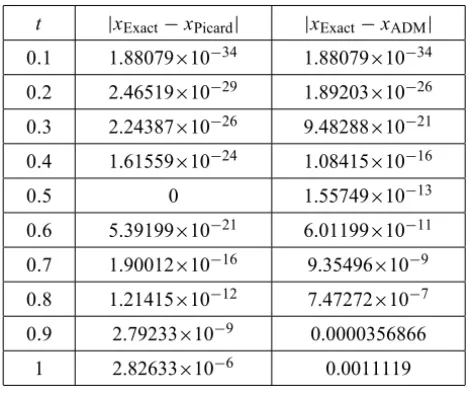
Table 2 shows a comparison between the absolute error of Picard (whenn=3) and ADM solutions (whenq =3).
t |xExact−xPicard| |xExact−xADM|
0.1 1.88079×10⁻³⁴ 1.88079×10⁻³⁴ 0.2 2.46519×10⁻²⁹ 1.89203×10⁻²⁶ 0.3 2.24387×10⁻²⁶ 9.48288×10⁻²¹ 0.4 1.61559×10⁻²⁴ 1.08415×10⁻¹⁶
0.5 0 1.55749×10⁻¹³
0.6 5.39199×10⁻²¹ 6.01199×10⁻¹¹ 0.7 1.90012×10⁻¹⁶ 9.35496×10⁻⁹ 0.8 1.21415×10⁻¹² 7.47272×10⁻⁷ 0.9 2.79233×10⁻⁹ 0.0000356866
1 2.82633×10⁻⁶ 0.0011119
Table 2 – Absolute error.
Example 3. Consider the following nonlinear QIE [9],
x(t)=t3+
1 4x(t)+
1 4
Z t
0
t+cos
x(s)
1+x2(s)
ds, (12)
Applying Picard method to equation (12), we get
xn(t) = t3+
1
4xn−1(t)+ 1 4
Z t
0
t+cos xn−1(s) 1+xn2−1(s)
!!
ds, n=1,2, . . . ,
x0(t) = t3.
and the solution will be,
Applying ADM to equation (12), we get
x0(t) = t3,
xn+1(t) =
1
4xn(t)+ 1 4
Z t
0
t+Ai−1(s)
ds, i ≥1.
whereAi are Adomian polynomials of the nonlinear term cos
x(s)
1+x2(s)
and the solution will be,
x(t)= q
X
i=0 xi(t).
Table 3 shows a caparison between ADM and Picard solutions.
t ADM solution Picard solution |xADM−xPicard|
0.1 0.0285275 0.0272762 0.00125125
0.2 0.0684798 0.0634398 0.00504
0.3 0.127128 0.115575 0.0115538
0.4 0.212929 0.191649 0.02128
0.5 0.335783 0.300627 0.0351563
0.6 0.507262 0.452542 0.05472
0.7 0.740798 0.65854 0.0822587
0.8 1.05195 0.930992 0.12096
0.9 1.45895 1.28389 0.175061
1 1.98343 1.73343 0.25
Table 3 – Absolute error.
Example 4. Consider the following nonlinear QIE [8],
x(t)=e−t +x(t) Z t
0
t2ln(1+s|x(s)|)
2e(t+s) ds, 0<t≤2. (13) Applying Picard method to equation (13), we get
xn(t) = e−t+xn−1(t)
Z t
0
t2ln(1+s|xn−1(s)|)
2e(t+s) ds, n =1,2, . . . ,x0(t)
= e−t.
and the solution will be,
Applying ADM to equation (13), we get
x0(t) = e−t,
xn+1(t) = xn(t)
Z t
0 t2A
i−1(s)
2e(t+s) ds, i ≥1.
where Ai are Adomian polynomials of the nonlinear term ln(1+s|x(s)|)and the solution will be,
x(t)= q
X
i=0 xi(t).
Table 4 shows a caparison between ADM and Picard solutions.
t ADM solution Picard solution |xADM−xPicard|
0.2 0.818926 0.818926 1.11022×10⁻¹⁶
0.4 0.671897 0.671897 0
0.6 0.552921 0.552921 0
0.8 0.456136 0.456136 0
1 0.376724 0.376724 0
1.2 0.31109 0.31109 0
1.4 0.256612 0.256612 2.77556×10⁻¹⁷
1.6 0.211338 0.211338 0
1.8 0.173748 0.173748 0
2 0.142602 0.142602 0
Table 4 – Absolute error.
6 Conclusion
We used two analytical methods to solve QIEs; Picard method and ADM, from the results in the tables we see that Picard method gives more accurate solution than ADM.
REFERENCES
[1] G. Adomian,Stochastic System. Academic Press (1983).
[3] G. Adomian, Nonlinear Stochastic Systems: Theory and Applications to Physics. Kluwer (1989).
[4] G. Adomian, R. Rach and R. Mayer, Modified decomposition. J. Appl. Math. Comput.,
23(1992), 17–23.
[5] K. Abbaoui and Y. Cherruault, Convergence of Adomian’s method Applied to Differential Equations.Computers Math. Applic.,28(1994) 103–109.
[6] G. Adomian, Solving Frontier Problems of Physics: The Decomposition Method. Kluwer (1995).
[7] J. Bana´s, M. Lecko and W.G. El-Sayed, Existence Theorems of Some Quadratic Integral Equation. J. Math. Anal. Appl.,227(1998), 276–279.
[8] J. Bana´s and A. Martinon,Monotonic Solutions of a quadratic Integral Equation of Volterra Type. Comput. Math. Appl.,47(2004), 271–279.
[9] J. Bana´s, J. Caballero, J. Rocha and K. Sadarangani, Monotonic Solutions of a Class of Quadratic Integral Equations of Volterra Type. Computers and Mathematics with Applica-tions,49(2005), 943–952.
[10] J. Bana´s, J. Rocha Martin and K. Sadarangani, On the solution of a quadratic integral equation of Hammerstein type.Mathematical and Computer Modelling,43(2006), 97–104. [11] J. Bana´s and B. Rzepka, Monotonic solutions of a quadratic integral equations of
frac-tional order.J. Math. Anal. Appl.,332(2007), 1370–11378.
[12] Y. Cherruault,Convergence of Adomian method.Kybernetes,18(1989), 31–38.
[13] Y. Cherruault, G. Adomian, K. Abbaoui and R. Rach, Further remarks on convergence of decomposition method.Int. J. of Bio-Medical Computing.,38(1995), 89–93.
[14] R.F. Curtain and A.J. Pritchard, Functional Analysis in Modern Applied Mathematics. Academic Press (1977).
[15] C. Corduneanu, Principles of Differential and integral equations. Allyn and Bacon. Hnc., New York (1971).
[16] A.M.A. El-Sayed, M.M. Saleh and E.A.A. Ziada, Numerical and Analytic Solution for Nonlinear Quadratic Integral Equations.Math. Sci. Res. J.,12(8) (2008), 183–191. [17] A.M.A. El-Sayed and H.H.G. Hashem, Carathéodory type theorem for a nonlinear
quad-ratic integral equation.Math. Sci. Res. J.,12(4) (2008), 71–95.
[18] A.M.A. El-Sayed and H.H.G. Hashem, Integrable and continuous solutions of nonlinear quadratic integral equation. Electronic Journal of Qualitative Theory of Differential Equa-tions,25(2008), 1–10.
[20] A.M.A. El-Sayed and H.H.G. Hashem,Weak maximal and minimal solutions for Hammer-stein and Urysohn integral equations in reflexive Banach spaces. Differential Equation and Control Processes,4(2008), 50–62.
[21] A.M.A. El-Sayed and H.H.G. Hashem, Monotonic solutions of functional integral and differential equations of fractional order. E.J. Qualitative Theory of Diff. Equ.,7(2009), 1–8.