ISSN 0101-8205 www.scielo.br/cam
Effect of Hall current on the velocity and
temperature distributions of Couette flow with
variable properties and uniform suction and injection
HAZEM ALI ATTIA
Department of Engineering Mathematics and Physics Faculty of Engineering, El-Fayoum University
El-Fayoum-63111, Egypt
E-mail: [email protected]
Abstract. The unsteady hydromagnetic Couette flow and heat transfer between two parallel
porous plates is studied with Hall effect and temperature dependent properties. The fluid is acted
upon by an exponential decaying pressure gradient and an external uniform magnetic field.
Uni-form suction and injection are applied perpendicularly to the parallel plates. Numerical solutions
for the governing non-linear equations of motion and the energy equation are obtained. The effect
of the Hall term and the temperature dependent viscosity and thermal conductivity on both the
velocity and temperature distributions is examined.
Mathematical subject classification: 76D05, 76M25.
Key words:Fluid Mechanics, nonlinear equations, Hall effect, numerical solution.
1 Introduction
The flow between parallel plates is a classical problem that has important ap-plications in magnetohydrodynamic (MHD) power generators and pumps, ac-celerators, aerodynamic heating, electrostatic precipitation, polymer technol-ogy, petroleum industry, purification of crude oil and fluid droplets and sprays. Hartmann and Lazarus [1] studied the influence of a transverse uniform magnetic field on the flow of a viscous incompressible electrically conducting fluid between
two infinite parallel stationary and insulating plates. The problem was extended in numerous ways. Closed form solutions for the velocity fields were obtained [2-5] under different physical effects. Some exact and numerical solutions for the heat transfer problem are found in [6, 7]. In the above mentioned cases the Hall term was ignored in applying Ohm’s law as it has no marked effect for small and moderate values of the magnetic field. However, the current trend for the application of magnetohydrodynamics is towards a strong magnetic field, so that the influence of electromagnetic force is noticeable [5]. Under these conditions, the Hall current is important and it has a marked effect on the magnitude and direction of the current density and consequently on the magnetic force. Tani [8] studied the Hall effect on the steady motion of electrically conducting and viscous fluids in channels. Soundalgekar et al. [9, 10] studied the effect of Hall currents on the steady MHD Couette flow with heat transfer. The temperatures of the two plates were assumed either to be constant [9] or varying linearly along the plates in the direction of the flow [10]. Abo-El-Dahab [11] studied the effect of Hall currents on the steady Hartmann flow subject to a uniform suction and injection at the bounding plates. Attia [12] extended the problem to the unsteady state with heat transfer.
In the present work, the unsteady Couette flow of a viscous incompressible electrically conducting fluid is studied with heat transfer. The viscosity and thermal conductivity of the fluid are assumed to vary with temperature. The fluid is flowing between two electrically insulating plates and is acted upon by an exponential decaying pressure gradient while a uniform suction and injection is applied through the surface of the plates. The upper plate is moving with a constant velocity while the lower plate is kept stationary. An external uniform magnetic field is applied perpendicular to the plates and the Hall effect is taken into consideration. The magnetic Reynolds number is assumed small so that the induced magnetic field is neglected [4]. The two plates are kept at two constant but different temperatures. This configuration is a good approximation of some practical situations such as heat exchangers, flow meters, and pipes that connect system components. Thus, the coupled set of the equations of motion and the energy equation including the viscous and Jouledissipation termsbecomes non-linear and is solved numerically using the finite difference approximations to obtain the velocity and temperature distributions.
2 Formulation of the problem
The fluid is assumed to be flowing between two infinite horizontal plates located at the y = ±hplanes. The two plates are assumed to be electrically insulating and kept at two constant temperaturesT1for the lower plate andT2for the upper plate withT2>T1. The upper plate is moving with a constant velocityUowhile
the lower plate is kept stationary. The motion is produced by an exponential decaying pressure gradientd P/d x = −Ge−αt in thex-direction, whereGand
αare constants. A uniform suction from above and injection from below, with
velocityvo, are applied att =0. A uniform magnetic fieldBois applied in the
condition at the plates implies that the fluid velocity has neither a z nor an x -component aty = ±h. The initial temperature of the fluid is assumed to be equal toT1. Since the plates are infinite in thexandz-directions, the physical quantities do not change in these directions and the problem is essentially one-dimensional.
The flow of the fluid is governed by the Navier-Stokes equation
ρDvE
Dt = − E∇p+ ∇ ∙(μ∇ Ev)+ EJ ∧ EBo (1)
whereρis the density of the fluid,μis the viscosity of the fluid, JEis the current density, andvEis the velocity vector of the fluid, which is given by
E
v=u(y,t)Ei+voEj+w(y,t)kE
If the Hall term is retained, the current density JEis given by the generalized Ohm’s law [4]
E
J =σ h
E
v∧ EBo−β JE∧ EBoi
(2)
whereσis the electric conductivity of the fluid andβis the Hall factor [4]. Using Eqs. (1) and (2), the two components of the Navier-Stokes equation are
ρ∂u ∂t +ρvo
∂u
∂y =Ge −αt +
μ∂ 2u ∂y2 +
∂μ ∂y
∂u
∂y −
σBo2
1+m2(u+mw) (3)
ρ∂w ∂t +ρvo
∂w ∂y =μ
∂2w ∂y2 +
∂μ ∂y
∂w ∂y −
σBo2
1+m2(w−mu) (4) where m is the Hall parameter given by m = σβBo. It is assumed that the
pressure gradient is applied att = 0 and the fluid starts its motion from rest. Thus
t =0:u =w=0 (5a)
Fort >0, the no-slip condition at the plates implies that
y = −h:u=w =0 (5b)
The energy equation describing the temperature distribution for the fluid is given by [19]
ρcp
∂T
∂t +ρcpvo
∂T
∂y =
∂ ∂y
k∂T
∂y +μ " ∂u ∂y 2 + ∂w ∂y 2#
+ σB 2
o
1+m2(u 2+
w2)
(6)
whereT is the temperature of the fluid,cpis the specific heat at constant
pres-sure of the fluid, andk is thermal conductivity of the fluid. The last two terms in the right-hand-side of Eq. (6) represent the viscous and Joule dissipations respectively.
The temperature of the fluid must satisfy the initial and boundary conditions,
t=0:T =T1 (7a)
t >0:T =T1, y = −h (7b)
t >0: T =T2, y=h (7c)
The viscosity of the fluid is assumed to vary with temperature and is defined as, μ = μof1(T). By assuming the viscosity to vary exponentially with temper-ature, the function f1(T) takes the form [7], f1(T) = exp(−a1(T −T1)). In some casesa1may be negative, i.e. the coefficient of viscosity increases with temperature [7, 15].
Also the thermal conductivity of the fluid is varying with temperature ask =
kof2(T). We assume linear dependence for the thermal conductivity upon the temperature in the formk =ko(1+b1(T −T1))[19], where the parameterb1 may be positive or negative [19].
The problem is simplified by writing the equations in the non-dimensional form. To achieve this define the following non-dimensional quantities,
ˆ
y= y
h, tˆ= tUo
h ,
ˆ
G = hG ρU2
o
, (uˆ,w)ˆ = (u, w)
Uo
, Tˆ = T −T1
T2−T1 ,
ˆ
f1(Tˆ)=e−a1(T2−T1) ˆ
T =e−aTˆ,ais the viscosity parameter,
ˆ
S =ρvoh/μois the suction parameter, H a2=σB2
oh2/μo, H ais the Hartmann number,
Pr=μocp/kois the Prandtl number, Ec=U2
o/cp(T2−T1)is the Eckert number.
In terms of the above non-dimensional quantities the velocity and energy equa-tions (3) to (7) read (the hats are dropped for convenience)
∂u
∂t + S
Re ∂u
∂y
=Ge−αt + 1 Re f1(T)
∂2u
∂y2 + 1 Re
∂f1(T) ∂y
∂u
∂y −
H a2
Re(1+m2)(u+mw) (8)
∂w ∂t +
S
Re ∂w
∂y
= 1 Re f1(T)
∂2w ∂y2 +
1 Re
∂f1(T) ∂y
∂w ∂y −
H a2
Re(1+m2)(w−mu)
(9)
t =0:u =w=0 (10a)
t >0: y = −1, u =w=0 (10b)
t>0: y=1, u =w=0 (10c)
∂T
∂t + S
Re ∂T
∂y =
1 Prf2(T)
∂2T ∂y2 +
1 Pr
∂f2(T) ∂y
∂T
∂y
+Ec f1(T) " ∂u ∂y 2 + ∂w ∂y 2#
+ Ec H a 2 Re(1+m2)(u
2+ w2)
(11)
t =0:T =0 (12a)
t>0:T =0, y = −1 (12b)
t >0: T =1, y=1 (12c)
boundary conditions (10) and (12) using finite difference approximations. The Crank-Nicolson implicit method is used [20]. Finite difference equations relat-ing the variables are obtained by writrelat-ing the equations at the mid point of the computational cell and then replacing the different terms by their second order central difference approximations in the y-direction. The diffusion terms are replaced by the average of the central differences at two successive time levels. The non-linear terms are first linearized and then an iterative scheme is used at every time step to solve the linearized system of difference equations. All calcu-lations have been carried out forG=5,α=1, Pr=1, Re=1, andEc=0.2. Step sides1t=0.001 and1y =0.05 for time and space respectively, are cho-sen and the scheme converges in at most 7 iterations at every time step. Smaller step sizes do not show any significant change in the results. Convergence of the scheme is assumed when any one ofu,w,T,∂u/∂y,∂w/∂yand∂T/∂yfor the last two approximations differ from unity by less than 10−6for all values of y in−1 < y < 1 at every time step. Less than 7 approximations are required to satisfy this convergence criteria for all ranges of the parameters studied here. The transient results obtained here converges to the steady state solutions given in [17] in the casem=0.
3 Results and Discussion
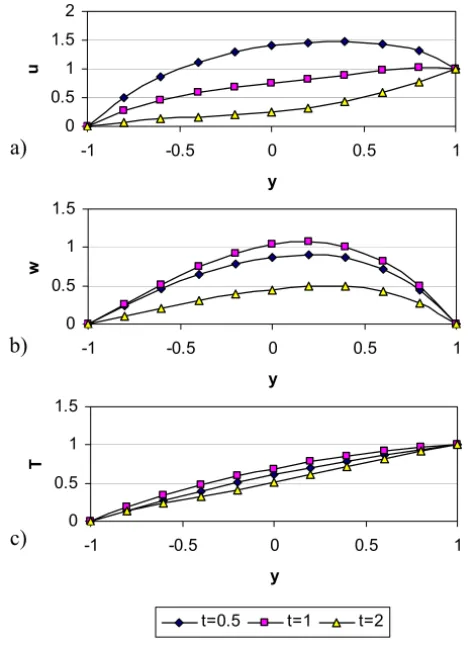
Figure 1 presents the velocity and temperature distributions as functions of y
for various values of timet starting fromt = 0 up to steady state. The figure is evaluated for H a = 1, m = 3, S = 0, a = 0.5 and b = 0.5. It is clear that the velocity and temperature distributions do not reaches the steady state monotonically. They increase with time up till a maximum value and decrease up to the steady state due to the influence of the decaying pressure gradient. The velocity componentureaches the steady state faster thanwwhich, in turn, reaches the steady state faster thanT. This is expected asu is the source ofw, while bothuandware sources ofT.
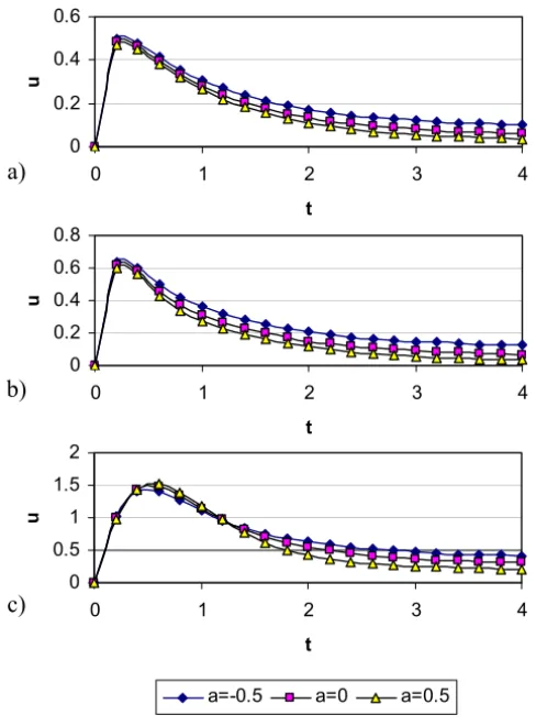
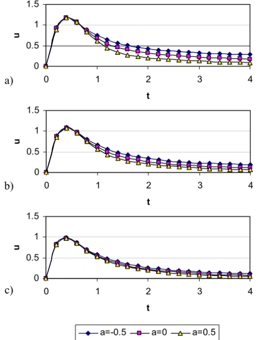
Figure 2 depicts the variation of the velocity componentuat the centre of the channel(y =0)with time for various values of the Hall parameterm and the viscosity parameter a and for b = 0 and H a = 3. The figure shows thatu
a)
0 0.5 1 1.5 2
-1 -0.5 0 0.5 1
b)
0 0.5 1 1.5
-1 -0.5 0 0.5 1
c)
0 0.5 1 1.5
-1 -0.5 0 0.5 1
t=0.5 t=1 t=2
Figure 1 – The evolution of the profile of: (a)u; (b)wand (c)T. (H a =3,m =3, a=0.5,b=0.5).
m decreases the effective conductivity (σ/(1+m2)) and hence the magnetic damping. The figure shows also how the effect ofaonudepends on the param-eterm. For small and moderate values ofa, increasinga decreasesu, however, for higher values ofm, increasinga increasesu. It is observed also from the figure that the time at whichu reaches its steady state value increases with in-creasingmwhile it is not greatly affected by changinga.
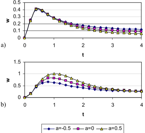
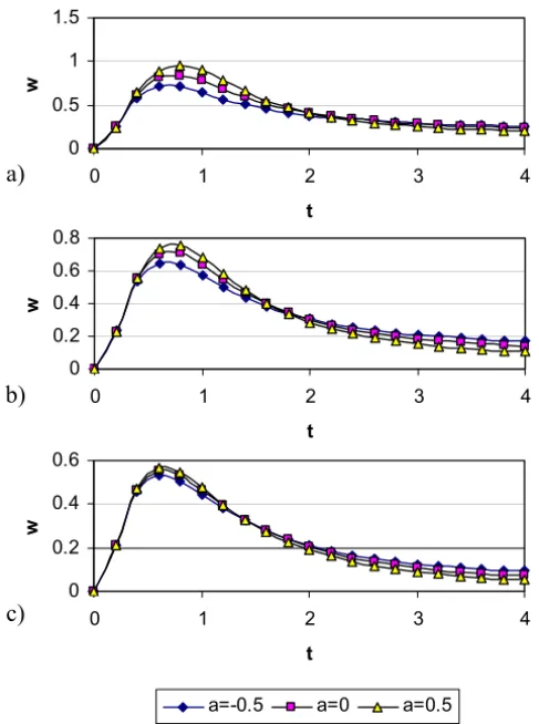
Figure 3 presents the variation of the velocity componentw at the centre of the channel(y = 0)with time for various values of m anda and for b = 0,
a)
0 0.2 0.4 0.6
0 1 2 3 4
b)
0 0.2 0.4 0.6 0.8
0 1 2 3 4
c)
0 0.5 1 1.5 2
0 1 2 3 4
a=-0.5 a=0 a=0.5
Figure 2 – The evolution ofu at y = 0 for various values ofa andm: (a)m = 0; (b)m=1 and (c)m=5. (H a=3,b=0).
Although the Hall effect is the source forw, a careful study of Figure 3 shows that, at small times, an increase in m produces a decrease in w. This can be understood by studying the term(−(w −mu)/(1+m2)) in Eq. (10), which is the source term ofw. At small timeswis very small and this term may be approximated to(mu/(1+m2)), which decreases with increasingmifm >1. Figure 3 shows also that for small values ofmthe effect ofaonwdepends on
t. For smallt, increasinga increasesw, but with time progress, increasinga
decreasesw.
a)
0 0.1 0.2 0.3 0.4 0.5
0 1 2 3 4
b)
0 0.5 1 1.5
0 1 2 3 4
a=-0.5 a=0 a=0.5
Figure 3 – The evolution ofwaty=0 for various values ofaandm: (a)m =1 and (b)m=5. (H a=3,b=0).
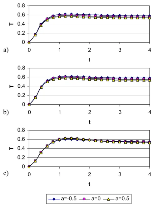
depends ont. Whenm>1, increasingmdecreasesT slightly at small times but increasesT at large times. This is because whent is small,u andware small and an increase inmresults in an increase inubut a decrease inw, so the Joule dissipation which is proportional also to (1/(1+m2)) decreases. When t is large, u and w increase with increasing m and so do the Joule and viscous dissipations. IncreasingaincreasesTdue to its effect on decreasing the velocities and the velocity gradients and the function f1.
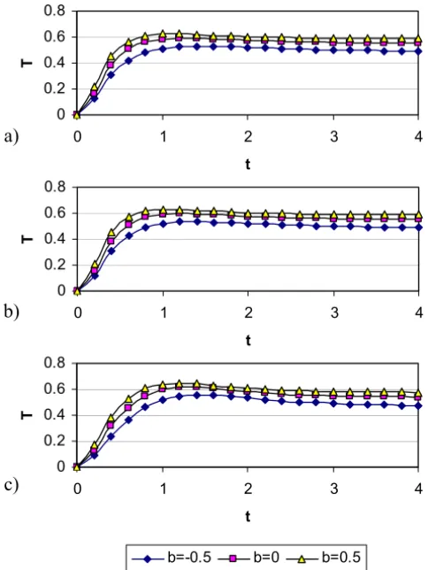
Figure 5 presents the evolution of T at the centre of the channel for various values ofm andbwhen a = 0, S =0 and H a = 3. The figure indicates that increasingbincreasesT and the time at which it reaches its steady state for all
m. This occurs because the centre of the channel acquires heat by conduction from the hot plate. The parameterbhas no significant effect onuorwin spite of the coupling between the momentum and energy equations.
a)
0 0.2 0.4 0.6 0.8
0 1 2 3 4
b)
0 0.2 0.4 0.6 0.8
0 1 2 3 4
c)
0 0.2 0.4 0.6 0.8
0 1 2 3 4
a=-0.5 a=0 a=0.5
Figure 4 – The evolution ofT aty = 0 for various values ofa andm: (a)m = 0; (b)m=1 and (c)m=5. (H a=3,b=0).
with increasingmas a result of decreasing the dissipations. On the other hand, increasingadecreasesTas a consequence of decreasing the dissipations. Table 2 shows the dependence ofT at the centre of the channel onmandbfora =0,
S = 0 and H a = 1. The dependence of T on m is explained by the same argument used for Table 1. Table 2 shows that increasingb increasesT since the centre gains temperature by conduction from hot plate. Table 3 shows the dependence ofT onaandbforH a =1 andm=3. Increasinga decreasesT
and increasingbdecreasesT.
Figures 6, 7, and 8 present the time development of the velocity componentsu
a)
0 0.2 0.4 0.6 0.8
0 1 2 3 4
b)
0 0.2 0.4 0.6 0.8
0 1 2 3 4
c)
0 0.2 0.4 0.6 0.8
0 1 2 3 4
b=-0.5 b=0 b=0.5
Figure 5 – The evolution ofT at y = 0 for various values ofb andm: (a)m = 0; (b)m=1 and (c)m=5. (H a=3,a=0).
T m=0.0 m=0.5 m=1.0 m=3.0 m=5.0 a= −0.5 0.5541 0.5511 0.5452 0.5338 0.5314 a= −0.1 0.5459 0.5439 0.5398 0.5310 0.5291 a =0.0 0.5435 0.5417 0.5382 0.5300 0.5281 a=0.1 0.5412 0.5396 0.5365 0.5289 0.5272 a=0.5 0.5325 0.5318 0.5301 0.5253 0.5240
T m=0.0 m=0.5 m=1.0 m=3.0 m=5.0 a= −0.5 0.5541 0.5511 0.5452 0.5338 0.5314 a= −0.1 0.5459 0.5439 0.5398 0.5310 0.5291 a =0.0 0.5435 0.5417 0.5382 0.5300 0.5281 a=0.1 0.5412 0.5396 0.5365 0.5289 0.5272 a=0.5 0.5325 0.5318 0.5301 0.5253 0.5240
Table 2 – Variation of the steady state temperatureT at y = 0 for various values of mandb(H a=1,a=0).
T m=0.0 m=0.5 m=1.0 m=3.0 m=5.0 b= −0.5 0.4805 0.4781 0.4732 0.4621 0.4596 b= −0.1 0.5329 0.5311 0.5273 0.5187 0.5167 b=0.0 0.5435 0.5417 0.5382 0.5300 0.5281 b=0.1 0.5528 0.5512 0.5478 0.5401 0.5383 b=0.5 0.5795 0.5781 0.5382 0.5690 0.5677
Table 3 – Variation of the steady state temperatureT at y = 0 for various values of aandb(H a=1,m=3).
various values of the suction parameterS and the viscosity variation parameter
awhen H a=3,m=3, andb=0. Figures 6 and 7 indicate that increasing S
a)
0 0.5 1 1.5
0 1 2 3 4
b)
0 0.5 1 1.5
0 1 2 3 4
c)
0 0.5 1 1.5
0 1 2 3 4
a=-0.5 a=0 a=0.5
Figure 6 – The evolution of u at y = 0 for various values of a and S: (a) S = 0; (b)S=1; (c)S=2. (H a=3,m=3,b=0).
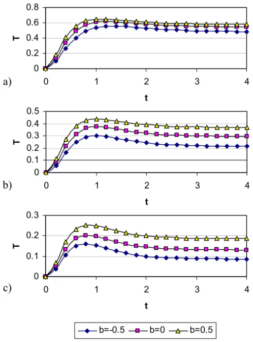
Note that the influence of increasing the parameterbonT is more apparent for higher values of suction velocity.
4 Conclusions
a)
0 0.5 1 1.5
0 1 2 3 4
b)
0 0.2 0.4 0.6 0.8
0 1 2 3 4
c)
0 0.2 0.4 0.6
0 1 2 3 4
a=-0.5 a=0 a=0.5
Figure 7 – The evolution ofw at y = 0 for various values of a and S: (a) S = 0; (b)S=1; (c)S=2. (H a=3,m=3,b=0).
are discussed. Introducing the Hall term gives rise to a velocity component win the z-direction and affects the main velocity u in thex-direction. It was found that the parametera has a marked effect on the velocity componentsu
andwfor all values ofm. On the other hand, the parameterbhas no significant effect onuorw.
REFERENCES
[1] J. Hartman and F. Lazarus,Kgl. Danske Videnskab. Selskab. Mat.-Fys. Medd., 15(6-7) (19315(6-7).
a)
0 0.2 0.4 0.6 0.8
0 1 2 3 4
b)
0 0.1 0.2 0.3 0.4
0 1 2 3 4
c)
0 0.05 0.1 0.15 0.2 0.25
0 1 2 3 4
a=-0.5 a=0 a=0.5
Figure 8 – The evolution of θ at y = 0 for various values ofa and S: (a) S = 0; (b)S=1; (c)S=2. (H a=3,m=3,b=0).
[3] R.A. Alpher,Heat transfer in magnetohydrodynamic flow between parallel plates. Interna-tional Journal of Heat and Mass Transfer,3(1961), 108.
[4] G.W. Sutton and A. Sherman, Engineering Magnetohydrodynamics. McGraw-Hill (1965).
[5] K. Cramer and S. Pai, Magnetofluid dynamics for engineers and applied physicists. McGraw-Hill (1973).
[6] S.D. Nigam and S.N. Singh,Heat transfer by laminar flow between parallel plates under the action of transverse magnetic field.Quart. J. Mech. Appl. Math.,13(1960), 85.
[7] H.A. Attia and N.A. Kotb,MHD flow between two parallel plates with heat transfer. Acta Mechanica,117(1996), 215–220.
a)
0 0.2 0.4 0.6 0.8
0 1 2 3 4
b)
0 0.1 0.2 0.3 0.4 0.5
0 1 2 3 4
c)
0 0.1 0.2 0.3
0 1 2 3 4
b=-0.5 b=0 b=0.5
Figure 9 – The evolution ofθ at y = 0 for various values ofb and S: (a) S = 0; (b)S=1; (c)S=2. (H a=3,m=3,a=0).
[9] V.M. Soundalgekar, N.V. Vighnesam and H.S. Takhar, Hall and ion-slip effects in MHD Couette flow with heat transfer.IEEE Transactions on Plasma Sciences,PS-7(3) (1979).
[10] V.M. Soundalgekar and A.G. Uplekar,Hall effects in MHD Couette flow with heat transfer.
IEEE Transactions on Plasma Science,PS-14(5) (1986).
[11] E.M.H. Abo-El-Dahab, Effect of Hall currents on some magnetohydrodynamic flow prob-lems. Master Thesis, Dept. of Math., Fac. of Science, Helwan Univ., Egypt (1993).
[12] H.A. Attia,Hall current effects on the velocity and temperature fields of an unsteady Hart-mann flow.Can. J. Phys.,76(1998), 739–746.
[13] H. Herwig and G. Wicken,The effect of variable properties on laminar boundary layer flow.
[14] K. Klemp, H. Herwig and M. Selmann,Entrance flow in channel with temperature depen-dent viscosity including viscous dissipation effects. Proceedings of the Third International Congress of Fluid Mechanics, Cairo, Egypt,3(1990), 1257–1266.
[15] H.A. Attia,Transient MHD flow and heat transfer between two parallel plates with temper-ature dependent viscosity.Mechanics Research Communications,26(1) (1999), 115–121.
[16] H.A. Attia and A.L. Aboul-Hassan,The effect of variable properties on the unsteady Hart-mann flow with heat transfer considering the Hall effect. Applied Mathematical Modelling, 27(7) (2003), 551–563.
[17] H.A. Attia,On the effectiveness of variation in the physical variables on the mhd steady flow between parallel plates with heat transfer.International Journal for Numerical Methods in Engineering, John Wiley & Sons, Ltd.,65(2) (2006), 224–235.
[18] H.A. Attia,On the effectiveness of variation in the physical variables on generaized Couette flow with heat transfer in a porous medium.Research Journal of Physics, Asian Network for Scientific Information (ANSI),1(1) (2007), 1–9.
[19] M.F. White, Viscous fluid flow, McGraw-Hill (1991).