ISSN 0101-8205 www.scielo.br/cam
A filter SQP algorithm without a feasibility
restoration phase*
CHUNGEN SHEN1,2, WENJUAN XUE3 and DINGGUO PU1
1Department of Mathematics, Tongji University, China, 200092
2Department of Applied Mathematics, Shanghai Finance University, China, 201209 3Department of Mathematics and Physics, Shanghai University of Electric Power, China, 200090
E-mail: [email protected]
Abstract. In this paper we present a filter sequential quadratic programming (SQP) algorithm for solving constrained optimization problems. This algorithm is based on the modified quadratic programming (QP) subproblem proposed by Burke and Han, and it can avoid the infeasibility of the QP subproblem at each iteration. Compared with other filter SQP algorithms, our algorithm does not require any restoration phase procedure which may spend a large amount of computation. We underline that global convergence is derived without assuming any constraint qualifications. Preliminary numerical results are reported.
Mathematical subject classification: 65K05, 90C30.
Key words:filter, SQP, constrained optimization, restoration phase.
1 Introduction
In this paper, we consider the constrained optimization problem:
(NLP)
min f(x)
s.t. cE(x)=0, cI(x)≤0, #753/08. Received: 10/III/08. Accepted: 03/IV/09.
wherecE(x)=(c1(x),c2(x),∙ ∙ ∙,cm1(x)) T,c
I(x)=(cm1+1(x),cm1+2(x),∙ ∙ ∙ , cm(x))T, E = {1,2,∙ ∙ ∙,m1}, I = {m1+1,m1+2,∙ ∙ ∙ ,m}, f : Rn → R andci : Rn → R,i ∈ E∪I are twice continuously differentiable functions. The feasible set of the problem (NLP) is denoted by X = {x ∈ Rn|cE(x) = 0, cI(x)≤0}.
The sequential quadratic programming (SQP) method has been widely used for solving the problem (NLP). It generates a sequence{xk}converging to the desired solution by solving the quadratic programming (QP) subproblem:
min q(d)= ∇f(xk)Td+ 12dTBkd s.t. ∇cE(xk)Td+cE(xk)=0,
∇cI(xk)Td+cI(xk)≤0,
kdk∞≤ρ,
(1.1)
whereρ >0 is the trust region radius,Bk ∈Rn×nis a symmetric positive definite matrix. At each iterationxk, the solution d of the QP subproblem is regarded as a trial step and the next trial iterate has the form xk +d. The acceptance of this trial step depends on whether the trial iteratexk +d makes some merit function descent. Generally, this merit function is a type of penalty function with some parameters whose adjustment can be problematic. Fletcher and Leyffer [7] proposed a trust region filter SQP method to solve the problem (NLP) instead of traditional merit function SQP methods. In addition, the computational results presented in Fletcher and Leyffer [7] are also very encouraging.
used also in conjunction with the line search strategy (see Wächter and Biegler [26, 27]); with interior point methods (see Benson, Shanno and Vanderbei [5]; Ulbrich, Ulbrich and Vicente [25]) and with the pattern search method (see Audet and Dennis [1]; Karas, Ribeiro, Sagastizábal and Solodov [15]).
However, all filter algorithms mentioned above include the provision for a feasibility restoration phase if the QP subproblem becomes inconsistent. Al-though any method (e.g. [3, 4, 16]) for solving a nonlinear algebraic system of equalities and inequalities can be used to implement this calculation, a large amount of computation may be spent. In this paper, we incorporate the filter technique with the modified QP subproblem for solving general constrained op-timization problems. The main feature of this paper is that there is no restoration phase procedure. Another feature is that global convergence of our algorithm is established without assuming any constraint qualifications.
This paper is organized as follows. In section 2, we describe how the modified QP subproblem is embedded in the filter algorithm. In section 3, it is proved that the algorithm is well defined, and is globally convergent to a stationary point. If Mangasarian-Fromowitz constraint qualification (MFCQ) holds at this stationary point, then it is a KKT point. In section 4, we report some numerical results.
2 Algorithm
It is well-known that the Karush-Kuhn-Tucker (KKT) conditions for the problem (NLP) are:
(
∇xL(x, λ, μ)=0, cE(x)=0, cI(x)≤0, λ≥0, λTcI(x)=0.
(2.2)
where
L(x, λ, μ)= f(x)+μTcE(x)+λTcI(x), (2.3) is the Lagrangian function,μ ∈ Rm1 andλ∈ Rm−m1 are the multipliers corre-sponding to the constraints of the problem (NLP).
subproblem instead of the subproblem (1.1). Before introducing the modified QP subproblem, we first solve the problem
min ql(d)=Pi∈E|∇ci(xk)Td+ci(xk)|
+ P
i∈Imax
0,∇ci(xk)Td+ci(xk) , s.t. kdk∞≤σk,
(2.4)
where the scalarσk >0 is used to restrictdin norm. Letd˜k denote the solution of (2.4). Ifσk ≤ ρandql(d˜k)=0, then the QP subproblem (1.1) is consistent. The problem (2.4) can be reformulated as a linear program
min d∈Rn,z
1∈Rm1, z2∈Rm−m1
emT1z1+em−mT 1z2
s.t. −z1≤ ∇cE(xk)Td+cE(xk)≤z1,
∇cI(xk)Td+cI(xk)≤z2, z2≥0,
kdk∞≤σk,
(2.5)
where vectors em1 = (1,1,∙ ∙ ∙,1)
T ∈ Rm1 and e
m−m1 = (1,1,∙ ∙ ∙,1) T ∈
Rm−m1.
Now we define thatsˉ(xk, σk)andrˉ(xk, σk)are equal toz2˜ and∇cE(xk)Td˜k+ cE(xk), respectively, where (d˜k,z1˜ ,z2˜ ) denotes the solution of (2.5). At each iteration, we generate the trial step by solving the modified QP subproblem
QP xk,Bk, σk, ρk
min q(d)= ∇f(xk)Td+12dTBkd s.t. ∇cE(xk)Td+cE(xk)= ˉr(xk, σk),
∇cI(xk)Td+cI(xk)≤ ˉs(xk, σk),
kdk∞≤ρk.
Here, at each iterate, we require thatρk be greater thanσk. So, the choice of σk depends onρk.
Define8(xk, σk)=
P
i∈E|ˉri(xk, σk)| +
P
i∈Isˉi(xk, σk), whererˉi(xk, σk)and
ˉ
feasible for the problem (2.4) and then ql(d˜k) ≤ ql(0) = V(xk), where the constraint violationV(x)is defined as
V(x)=X
i∈E
|ci(x)| +
X
i∈I max
0,ci(x) .
Therefore,8(xk, σk)≤V(xk).
Let d denote the solution of QP(xk,Bk, σk, ρk). Let the trial point be xˆ = xk+d. The KKT conditions for the subproblem QP(xk,Bk, σk, ρk)are
∇f(xk)+Pi∈Iλk,i∇ci(xk)+Pi∈Eμk,i∇ci(xk)+Bkd+λuk −λlk=0,
λk,i(∇ci(xk)Td+ci(xk)− ˉsi(xk, σk))=0, i∈I,
(d−ρken)Tλuk =0, (d+ρken)Tλlk =0,
∇ci(xk)Td+ci(xk)− ˉri(xk, σk)=0, i ∈E,
∇ci(xk)Td+ci(xk)≤ ˉsi(xk, σk), i∈I, kdk∞≤ρk,
λk,i ≥0, i ∈I, λuk,j ≥0, λlk,j ≥0, j ∈ {1,2,∙ ∙ ∙,n},
(2.6)
whereen = (1,1,∙ ∙ ∙ ,1)T ∈ Rn, μk ∈ Rm1, λk ∈ Rm−m1, λlk ∈ Rn and λuk ∈Rn.
In our filter, we consider pairs of values(V(x), f(x)). Definitions 1–4 below are very similar to those in [7, 8].
Definition 1. The iterate xk dominates the iterate xl if and only if V(xk) ≤ V(xl)and f(xk)≤ f(xl). And it is denoted byxk xl.
Thus, ifxk xl, the latter is of no real interest to us sincexkis at least as good asxl with respect to the objective function’s value and the constraint violation. Furthermore, ifxk xl, we say that the pair(V(xk), f(xk))dominates the pair (V(xl), f(xl)).
Definition 2. Thekth filter is a list of pairs(V(xl), f(xl)) l<k, such that no pair dominates any other.
LetFk denote the indices in thekth filter, i.e., Fk =
Filter methods accept a trial pointxˆ = xk +d if its corresponding pair(V(xˆ), f(xˆ))is not dominated by any other pair in thekth filter, neither the pair corre-sponding toxk, i.e.,(V(xk), f(xk)).
In a filter algorithm, one accepts a new pair(V(xˆ), f(xˆ))if it cannot be domi-nated by other pairs in the current filter. Although the definition of filter is simple, it needs to be refined a little in order to guarantee the global convergence.
Definition 3. A new trial pointxˆ is said to be “acceptable toxl”, if
V(xˆ)−V(xl)≤ −γ1V(xˆ), (2.7a) or f(xˆ)− f(xl) <−γ2V(xˆ), (2.7b) is satisfied, whereγi ∈ 0,12
, i =1,2 are two scalars.
Definition 4. A new trial point xˆ is said to be “acceptable to thekth filter” if
ˆ
x is acceptable toxl for alll∈Fk.
Therefore, to accept a new pair into the current filter, we should test the con-ditions defined in Definition 4. If the new trial pointxˆ is acceptable in the sense of Definitions 3 and 4, we may wish to add the corresponding pair to the filter. Meanwhile, any pair in the current filter dominated by the new pair is removed. In order to restrictV(xk), it still needs an upper bound condition for accepting a point. The trial pointxˆ satisfies the upper bound condition if
V(xˆ)≤Uk (2.8) holds, whereUk is a positive scalar. HereUk is updated at each iteration and it may converge to zero for some instances. We aim to control the constraint violation by settingUk. In current iteration k, if a trial step is accepted and
8(xk, σk) = 0, then we will keepUk unchanged in next iteration. Otherwise we will reduceUk in next iteration. The detailed information about the update ofUkis given in Algorithm 2.1.
Denote
1q(d)=q(0)−q(d)= −∇f(xk)Td− 1 2d
T
as the quadratic reduction of f(x), and
1f(d)= f(xk)− f(xk +d) (2.10) as the actual reduction of f(x). In our algorithm, if a trial point xk +d is acceptable to the current filter andxk, and
1q(d) >0, (2.11)
the sufficient reduction criterion of the objective function f should be satis-fied, i.e.,
1f(d)≥η1q(d), η∈0,1
2
. (2.12)
Now we are in the position to state our filter SQP algorithm.
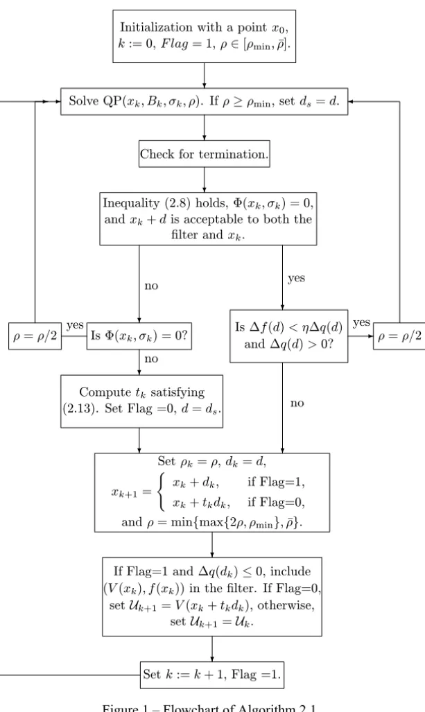
Algorithm 2.1.
Step 1. Initialization.
Given initial point x0, parametersη ∈ 0,12,γ1 ∈ 0,12
, γ2 ∈ 0,12
,γ ∈ (0,0.1),r ∈ (0,1),U0 >0,ρmin >0,ρ > ρˉ min,ρ ∈ [ρmin,ρˉ],σ0 ∈(γρ, ρ). Setk=0, Flag=1, putkintoFk.
Step 2. Compute the search direction.
Compute the search direction d from the subproblem QP(xk,Bk, σk, ρ). If ρ≥ρmin, setds =dand8s =8(xk, σk).
Step 3. Check for termination. Ifd =0 andV(xk)=0, then stop;
Else ifV(xk) >0 and8(xk, σk)−V(xk)=0, then stop. Step 4. Test to accept the trial point.
4.1.Check acceptability to the filter.
If the upper bound condition (2.8) holds forxˆ =xk+d,8(xk, σk)=0, and xk+d is acceptable to both thekth filter andxk, then go to 4.3.
4.2.Computetk, the first numbertof the sequence{1,r,r2,∙ ∙ ∙,}satisfying V xk+tkds
−V xk
≤tkη 8s −V(xk)
. (2.13) Set Flag=0,d =ds, and go to 4.4.
4.3.Check for sufficient reduction criterion.
If1f(d) < η1q(d)and1q(d) >0, thenρ = 12ρ and chooseσk ∈(γρ, ρ), and go to Step 2;
otherwise go to 4.4.
4.4.Accept the trial point. Set ρk =ρ, dk =d, xk+1=
(
xk+dk, if Flag=1, xk+tkdk, if Flag=0, andρ =minmax{2ρ, ρmin},ρˉ .
Step 5. Augment the filter if necessary.
If Flag=1 and1q(dk)≤0, then include(V(xk), f(xk))in thekth filter. If Flag=0, then set Uk+1 = V(xk +tkdk); otherwise, set Uk+1 = Uk and leave the filter unchanged.
Step 6. Update.
ComputeBk+1. Setσk+1∈(γρ, ρ)andk :=k+1, Flag=1, go to Step 2.
Remark 1. The role ds in Step 2 is to record a trial step d with ρ ≥ ρmin. By Step 4.1, we know that if8(xk, σk) > 0, then both conditions in Step 4.1 are violated. A trial iteratexk+d with8(xk, σk) > 0 may be considered as a “worse” step which may be far away from the feasible region. So Step 4.2 is executed to reduce the constraint violation. The stepds is used in Step 4.2 due to the descent property ofds proved by Lemma 3.4. In addition, it should be interpreted that, at the beginning of iterationk, the pair(V(xk), f(xk))is not in the current filter, butxk must be acceptable to the current filter.
Initialization with a pointx0,
k:= 0,F lag= 1,ρ∈[ρmin,ρ¯].
Solve QP(xk, Bk, σk, ρ). Ifρ≥ρmin, setds=d.
Check for termination.
Inequality (2.8) holds, Φ(xk, σk) = 0,
andxk+dis acceptable to both the
filter andxk.
no yes
Is Φ(xk, σk) = 0?
ρ=ρ/2 yes
no
Computetksatisfying
(2.13). Set Flag =0,d=ds.
Is ∆f(d)< η∆q(d) and ∆q(d)>0?
yes
ρ=ρ/2
no
Setρk=ρ,dk=d,
xk+1= (
xk+dk, if Flag=1,
xk+tkdk, if Flag=0,
andρ= min{max{2ρ, ρmin},ρ¯}.
If Flag=1 and ∆q(dk)≤0, include
(V(xk), f(xk)) in the filter. If Flag=0,
setUk+1=V(xk+tkdk), otherwise,
setUk+1=Uk.
Setk:=k+ 1, Flag =1.
the radiusρ is not less than ρmin. At each iteration, the first trial radius ρ is greater than or equal to ρmin. Subsequently, trial radiusρ may not stop de-creasing until either the filter acceptance criteria are satisfied or Step 4.2 is executed. Hence,ρ may be less than ρmin during the execution process of the loops 2-(4.1)-2 and 2-(4.3)-2.
As for proving global convergence, we use the terminology firstly introduced by Fletcher, Leyffer and Toint [8]. We call d an f -type stepif 1q(d) > 0, indicating that then the sufficient reduction criterion (2.12) is required. If d is accepted as the final step dk in thekth iteration, we refer to k as an f -type iteration.
Similarly, we call d a V-t ype step if 1q(d) ≤ 0. Ifd is accepted as the final stepdk in iterationk, we refer tokas aV -type iteration. In addition, ifxk is generated by Step 4.2, we also refer to it as aV -type iteration.
If f(xk+1) < f(xk), then we regard the stepdkas an f monotone step. Obvi-ously, an f -type stepmust be an f monotone step.
3 Global convergence
In this section, we prove the global convergence of Algorithm 2.1. Firstly, we give some assumptions:
(A1) Let{xk}be generated by Algorithm 2.1 and{xk},{xk+dk}are contained in a closed and bounded setSofRn;
(A2) All the functions f,ci, i ∈ E ∪I are twice continuously differentiable onS.
(A3) The matrixBk is uniformly positive definite and bounded for allk.
Remark 3. Assumption (A1) is reasonable. It may be forced if, for example, the original problem involves a bounded box among its constraints.
Remark 4. A consequence of Assumption (A3) is that there exist constants
δ,M>0, independent ofksuch thatδkyk2≤ yTB
ky≤ Mkyk2for ally ∈Rn. Assumptions (A1) and (A2) imply boundedness ofk∇2c
k∇2f(x)kon S. Without loss of generality, we may assumek∇2c
i(x)k ≤ M, i∈E∪I,k∇2f(x)k ≤ M,∀x ∈ S.
Lemma 3.1. Assume x is not a stationary point of V in the sense thatˉ 0 ∈/ ∂V(xˉ), where∂V denotes the Clarke subdifferential of V . Then there exists a scalarǫ >ˉ 0and a neighborhood N(xˉ)ofx, such thatˉ 8(x, σ )−V(x) < − ˉǫ
for allσ ≥γρminand all x∈ N(xˉ).
Proof. By [2, Lemma 2.1], 0 ∈/ ∂V(xˉ) implies 8(xˉ, γρmin)−V(xˉ) < 0, whereγ andρmin are from Algorithm 2.1. By the continuity of the function
8(∙, γρmin)−V(∙)onRn, there exists a neighborhoodN(xˉ)and a scalarǫ >ˉ 0 such that8(x, γρmin)−V(x) <− ˉǫ wheneverx ∈ N(xˉ). The conditionσ ≥
γρmintogether with the definition of8yields8(x, σ )−V(x)≤8(x, γρmin)− V(x). Therefore, 8(x, σ )− V(x) < − ˉǫ holds for all σ ≥ γρmin and all
x ∈ N(xˉ).
Remark 5. It can be seen that ǫˉ depends on xˉ such that 0 ∈/ ∂V(xˉ) (i.e.,
ˉ
ǫ= ˉǫ(xˉ)), because it must satisfy8(xˉ, σ )−V(xˉ) <− ˉǫ.
Lemma 3.2. Let dk = 0be a feasible point of QP(xk,Bk, σk, ρk). Then xk is a stationary point of V(x). Moreover, if xk ∈ X , then xk is a KKT point of the problem (NLP).
Proof. Sincedk =0 implies8(xk, σk)−V(xk)=0, it follows from [2, Lem-ma 2.1] thatxk is a stationary point ofV(x). IfV(xk)=0 anddk = 0, then it follows from [2, Lemma 2.2] thatxk is a KKT point for the problem (NLP).
Lemma 3.3. Let Assumptions (A1)-(A3) hold and d be a feasible point of the subproblem QP(x,B, σ, ρ), then we have
V(x+td)−V(x)≤t(8(x, σ )−V(x))+1
2t 2mn M
Proof. By Taylor Expansion formula, the feasibility ofdand Assumption (A2), we have that fori ∈E andt ∈ [0,1],
|ci(x +td)| = |ci(x)+t∇ci(x)Td + 1 2t
2
dT∇2ci(zi)d|
≤ (1−t)|ci(x)| +t|(ci(x)+ ∇ci(x)Td)| + 1 2t
2
n Mρ2, (3.15) and fori ∈Iandt ∈ [0,1],
ci(x +td) = ci(x)+t∇ci(x)Td+ 1 2t
2
dT∇2ci(zi)d
≤ (1−t)ci(x)+t(ci(x)+ ∇ci(x)Td)+ 1 2t
2n Mρ2, (3.16)
where the vectorzi is betweenx andx +td. The term 12t2n Mρ2in (3.15) and (3.16) is derived because
|dT∇2ci(zi)d| ≤n Mρ2, where we use thatk ∙ k2≤nk ∙ k2
∞. Formulae (3.15) and (3.16) combining with definitions ofV(x)and8(x, σ )yield (3.14).
The following lemma shows that the loop in Step 4.2 is finite.
Lemma 3.4. Let Assumptions(A1)-(A3)hold,η∈ 0,12andx satisfiesˉ 0∈/ ∂V(xˉ). Then, there exist a scalartˉ > 0 and a neighborhood N(xˉ)of x suchˉ
that for any x ∈ N(xˉ)and any d feasible for the problem QP(x,B, σ, ρ)with
γρmin≤σ ≤ρ ≤ ˉρ, it holds that
V(x +td)−V(x)≤tη(8(x, σ )−V(x)), (3.17) for all t ∈(0,tˉ].
Proof. It follows from Lemma 3.1 that there exists a neighborhoodN(xˉ)and
ˉ
ǫ(xˉ) > 0 such that8(x, σ )−V(x) < − ˉǫ(xˉ)wheneverx ∈ N(xˉ). Combin-ing this with (3.14), we have
V(x +td)−V(x)≤tη(8(x, σ )−V(x))−t(1−η)ǫ(ˉ xˉ)+1
2t 2
Hence, the inequality (3.17) holds for allt ∈(0,tˉ(xˉ)], where
ˉ
t(xˉ):= 2(1−η)ǫ(ˉ xˉ)
mn Mρˉ2 .
Hence, if 0 ∈/ ∂V(xk), (2.13) follows taking xˉ = x = xk and d = ds. It implies that the loop in Step 4.2 is finite.
The following lemma shows that the iterate sequence{xk}approaches a sta-tionary point of V(x) when Step 4.2 of Algorithm 2.1 is invoked infinitely many times.
Lemma 3.5 If Step4.2of Algorithm2.1is invoked infinitely many times, then there exists an accumulation pointx ofˉ {xk}such that the sequence{Uk} con-verges to V(xˉ), where0∈∂V(xˉ), i.e.,x is a stationary point of Vˉ (x).
Proof. Since Step 4.2 is invoked infinitely many times. By Step 5Uk+1 is reset byV(xk+tkdk)infinitely. From Step 2 and 4.2, we note that if Step 4.2 is invoked at iterationk, the radiusρin QP(xk,Bk, σk, ρ)associated withds is greater than or equal toρmin. DefineK= {k |Uk+1is reset byV(xk+tkdk)}. Obviously,Kis an infinite set. The inequality (2.13) ensures V(xk+1)=Uk+1 for allk ∈K. The upper bound condition (2.8) ensuresV(xk+1)≤Uk =Uk+1 for allk ∈/K. Therefore,V(xk)≤Ukfor allk. This together with (2.13) yields Uk+1 ≤ V(xk) ≤ Uk for allk ∈ K. For k ∈/ K, Uk+1 = Uk. Therefore,
{Uk}is a monotonically decreasing sequence and also has a lower bound zero. Then there exists an accumulation pointxˉ of{xk}such that{Uk+1}K →V(xˉ). If 0 ∈/ ∂V(xˉ), by Lemma 3.1, there exists a neighborhood N(xˉ) of xˉ and
ˉ
ǫ(xˉ) >0, such that
8(xk, σk)−V(xk) <− ˉǫ(xˉ), (3.18) wheneverxk ∈ N(xˉ). This together with (2.13) yields
Uk+1−Uk ≤Uk+1−V(xk) <−tkηǫ(ˉ xˉ), (3.19) fork ∈Kandxk ∈ N(xˉ). By the mechanism of Algorithm 2.1 and Lemma 3.4, we havetk ≥rtˉ(xˉ). It follows with (3.19) that
fork ∈ Kandxk ∈ N(xˉ). Lettingk ∈Ktend to infinity in above inequality, the limit in the left-hand side is zero while the limit in the right-hand side is less than zero, which is a contradiction. Therefore 0∈∂V(xˉ).
Lemma 3.6. Consider sequences {V(xk)} and {f(xk)} such that f(xk) is monotonically decreasing and bounded below. If for all k, either V(xk+1)− V(xk)≤ −γ1V(xk+1)or f(xk)− f(xk+1)≥γ2V(xk+1)holds, where constants
γ1andγ2are from(2.7a)and(2.7b), then V(xk)→0, for k→ +∞.
Proof. See [8, Lemma 1].
Lemma 3.7. Suppose Assumptions(A1)-(A3)hold. If there exists an infinite sequence of iterates{xk}on which (V(xk),f(xk)) is added to the filter, where V(xk) >0and{f(xk)}is bounded below, then V(xk)→0as k→ +∞.
Proof. Since inequalities (2.7a) and (2.7b) are the same as [8, (2.6)], the con-clusion follows from Lemma 3.6 and [8, Corollary].
Lemma 3.8. Suppose Assumptions(A1)-(A3)hold. Let d be a feasible point of QP(xk,Bk, σk, ρ). If8(xk, σk)=0, it then follows that
1f(d)≥ △q(d)−nρ2M, (3.20) V(xk +d)≤
1 2mnρ
2M. (3.21)
Proof. The proof of this lemma is very similar to the proof [8, Lemma 3]. By Taylor’s theorem, we have
f(xk +d)= f(xk)+ ∇f(xk)Td+ 1 2d
T∇2f
(y)d,
whereydenotes some point on the line segment fromxktoxk+d. This together with (2.9) and (2.10) implies
1f(d)= △q(d)+ 1
2d T B
k− ∇2f(y)
Then (3.20) follows from the boundedness of∇2f(y)and B
k, andkdk∞ ≤ρ. Since 8(xk, σk) = 0, QP(xk,Bk, σk, ρ) reduces to (1.1). For i ∈ E ∪I, it follows that
ci(xk+d)=ci(xk)+ ∇ci(xk)Td+ 1 2d
T∇2c i(yi)d,
whereyi denotes some point on the line segment fromxktoxk+d. By feasibil-ity ofd,
|ci(xk+d)| ≤ 1 2nρ
2M, i ∈E and
ci(xk +d)≤ 1 2nρ
2M, i∈ I.
follow in a similar way. It follows with the definition of V(x) that (3.21)
holds.
Lemma 3.9. Suppose Assumptions(A1)-(A3)hold. Let d be a feasible point of QP(xk,Bk, σk, ρ)with8(xk, σk)=0. Then xk+d is acceptable to the filter ifρ2≤ 2τk
mn M(1+γ1), whereτk :=k∈Fmink{V(xk)}.
Proof. It follows from (3.21) that V(xk +d)−τk ≤ −γ1V(xk +d) holds ifρ2 ≤ 2τk
mn M(1+γ1). By the definition ofτk, (2.7a) is satisfied. Hence xk +d
is acceptable to the filter.
In order to prove that the iterate sequence generated from Algorithm 2.1 con-verges to a KKT point for the problem (NLP), some constraint qualification should be required, such as the well-known MFCQ. Thus we review its defini-tion as follows.
Definition 5(See [2]). MFCQ is said to be satisfied at x, with respect to the underlying constraint systemcE(x)=0,cI(x)≤0, if there is az ∈Rnsuch that the gradients∇ci(x), i ∈Eare linearly independent and the following systems
∇ci(x)Tz=0, i ∈E,
∇ci(x)Tz <0, i ∈
Proposition 3.10. Suppose that MFCQ is satisfied at x∗∈ X , then there exists a neighborhood N(x∗)of x∗such that
1. MFCQ is satisfied at every point in N(x∗)∩X ; 2. inequality
sup k
kμkk1+ kλkk1:xk∈ N(x∗), σk ∈(ρmin, ρk), ρk∈(ρmin,ρˉ] <+∞.
holds, where the vectorsλk,μkgenerated by QP(xk,Bk, σk, ρk)are multiplier
vectors associated with xk ∈N(x∗).
Proof. The first result is established in [20, Theorem 3]. The second result is
established in [2, Theorem 5.1].
If MFCQ does not hold at a feasiblex∗, then the second statement of Propo-sition 3.10 cannot be guaranteed. All feasible points of the problem (NLP) at which MFCQ does not hold will be called non-MFCQ points.
The following lemma shows that (1.1) is consistent when xk approaches a feasible point at which MFCQ holds and both the quadratic reduction and the actual reduction of the objective function have sufficient reduction. Its proof is similar to that of [8, Lemma 5].
Lemma 3.11. Suppose Assumptions(A1)-(A3)hold and let x∗∈S be a feasi-ble point of profeasi-blem (NLP) at which MFCQ holds but which is not a KKT point. Then there exists a neighborhood N◦of x∗ and positive constantsǫ, ν andκ, such that for all xk ∈S∩N◦and allρfor which
νV(xk)≤ρ≤κ, (3.22) it follows that QP(xk,Bk, σk, ρ)with8(xk, σk)=0has a feasible solution d at which the predicted reduction satisfies
△q(d)≥ 1
3ρǫ, (3.23)
the sufficient reduction condition(2.12)holds, and the actual reduction satisfies
Proof. Sincex∗is a feasible point at which MFCQ holds but it is not a KKT point, it follows that the vectors∇ci(x∗), i ∈ E are linearly independent, and there exists a vectors∗that satisfies
∇ f(x∗)Ts∗<0, (3.25)
∇ci(x∗)Ts∗=0, i∈E, (3.26)
∇ci(x∗)Ts∗<0, i∈A(x∗)= {i:ci(x∗)=0, i ∈I}, (3.27)
where ks∗k = 1. Let ∇cE(xk)+ = ∇cE(xk)T∇cE(xk)
−1
∇cE(xk)T and
∇cE(xk) denote the matrix with columns ∇ci(xk), i ∈ E. It follows from linear independence and continuity that there exists a neighborhood of x∗ in which ∇cE(xk)+ is bounded. Let P = −∇cE(xk)+TcE(xk) and s = I −
∇cE(xk)∇cE(xk)+
s∗/k I − ∇c
E(xk)∇cE(xk)+
s∗k if E is not empty, other-wise P = 0 ands = s∗. Let p = kPk. It follows from (3.25) and (3.27) by continuity that there exists a (smaller) neighborhoodN∗ and a constantǫ >0 such that
∇f(xk)Ts∗<−ǫ and ∇ci(xk)Ts∗<−ǫ, i ∈A(x∗), (3.28) when xk ∈ N∗. By definition of P, it follows that p = O(V(xk)), and thus we can choose the constantνin (3.22) sufficiently large so thatρ > p for all xk ∈N∗.
We now consider the solution of (1.1). The line segment defined by
dα = P+α(ρ−p)s, α ∈ [0,1], (3.29)
for a fixed value ofρ > p. Sinceρ > p, and Pandsare orthogonal, it implies
kd1k∞≤ kd1k =pp2+(ρ−p)2=pρ2−2ρp+2p2 ≤ρ. (3.30) From (3.29) and the definitions of P, s, dα satisfies the equality constraints
cE(xk)+ ∇cE(xk)Tdα =0 of (1.1) for allα∈ [0,1].
Ifxk ∈ N∗∩Sandi ∈ I\A(x∗), then there exists positive constantscˉ and
ˉ
a, independent ofρ, such that
for all vectorss such thatksk∞ ≤ 1, by the continuity ofci(xk)and bounded-ness of∇ci(xk)on S. It follows that
ci(xk)+ ∇ci(xk)Td ≤ − ˉc+ρaˉ, i ∈I\A(x∗)
for all vectors d such thatkdk∞ ≤ ρ. Therefore, inactive constraints do not affect the solution of (1.1) ifρsatisfiesρ≤ ˉc/a.ˉ
For active inequality constraintsi ∈A(x∗), it follows from (3.28) and (3.29) thatci(xk)+ ∇ci(xk)Td1=ci(xk)+ ∇ci(xk)TP+(ρ−p)∇ci(xk)Ts ≤ci(xk)+
∇ci(xk)TP−(ρ− p)ǫ ≤ 0 if ρ ≥ p+(ci(xk)+ ∇ci(xk)TP)/ǫ. We obtain from the definition of Pthat
∃ν0 >0 s.t. 1
ǫ ci(xk)+ ∇ci(xk) TP
≤ν0V(xk).
Thus we can choose the constantν in (3.22) sufficiently large so thatci(xk)+
∇ci(xk)Td1 ≤ 0, i ∈ A(x∗). Therefore d1 is feasible in (1.1) with respect to the active inequality constraints, and hence to all the constraints by above results. Combining with the fact that (1.1) is equivalent to QP(xk,Bk, σk, ρ) with 8(xk, σk) = 0, we obtain that QP(xk,Bk, σk, ρ) with 8(xk, σk) = 0 is consistent for allxk ∈N∗and allρsatisfying (3.22) for any value ofκˉ ≤ ˉc/a.ˉ Next we aim to obtain a bound on the predicted reduction1q(d). We note thatq(0)−q(d1) = −∇f(xk)T(P +(ρ − p)s)− 12d1TBkd1. Using (3.28), bounds onBkandP, andρ > p=O(V(xk)), we have
q(0)−q(d1) ≥ (ρ−p)ǫ−1
2ρ 2n M+
O(V(xk))
= ρǫ−1
2ρ
2n M+O(V(x k)). Ifρ < n Mǫ , thenq(0)−q(d1) ≥ 1
2ρǫ +O(V(xk)). Sinced1 is feasible and p=O(V(xk)), it follows that the predicted reduction (2.9) satisfies
1q(d)≥1q(d1)≥ 1
2ρǫ+O(V(xk))≥ 1
2ρǫ−ξV(xk)
for someξ sufficiently large and independent ofρ. Hence, (3.23) is satisfied if
Next we aim to prove (3.24). By (3.20) and (3.23), we have
1f(d) 1q(d) ≥1−
nρ2M
1q(d) ≥1−
3nρ2M
ρǫ =1−
3nρM
ǫ .
Then, ifρ ≤(1−η)ǫ/(3n M), it follows that (2.12) holds. By (2.12), (3.21) and (3.23), we have f(xk)− f(xk+d)−γ2V(xk+d)=1f(d)−γ2V(xk+d)≥ 1
3ηρǫ− 1 2γ2mnρ
2M ≥ 0 ifρ ≤ 2
3ηǫ/(γ2mn M). Therefore, we may define the constantκˉ in (3.22) to be the least of 23ηǫ/(γ2mn M)and the values (1−η)ǫ/ (3n M),ρ < n Mǫ andcˉ/a, as required earlier in the proof.ˉ
Lemma 3.12. Suppose Assumptions(A1)-(A3)hold and let x∗∈S be a feasi-ble point of profeasi-blem (NLP) at which MFCQ holds but which is not a KKT point. Then there exists a neighborhood N◦of x∗and a positive constantν, such that for all xk ∈ S∩N◦, allρand allσk for which
νV(xk)≤σk < ρ, (3.31)
it follows that8(xk, σk)=0and QP(xk,Bk, σk, ρ)has a feasible solution d at which the predicted reduction satisfies
△q(d) >0. (3.32)
Proof. By Lemma 3.11, there exists a neighborhood N1 of x∗ and positive constantsν,κˉ such that for allxk ∈ S∩N◦and allρandσkfor whichνV(xk)≤ ρ ≤ ˉκ, it follows that the QP subproblem (1.1) has a feasible solution d at which the predicted reduction satisfies (3.32). Since the global optimality of d ensures that 1q(d) decreases monotonically as ρ decreases, the predicted reduction satisfies (3.32) wheneverνV(xk)≤ρ.
From the earlier proof, if νV(xk) ≤ σk ≤ ˉκ, we also have that the QP sub-problem (1.1) is consistent by takingρ = σk. It means that the problem (2.4) has the optimal value 0. Ifσkincreases to a value larger thanκˉ, then the feasible region of the problem (2.4) withρ = σk is also enlarged correspondingly and the optimal value is still 0. Therefore,8(xk, σk)=0 wheneverνV(xk)≤σk.
The above two conclusions complete the proof.
Lemma 3.13. Suppose Assumptions(A1)-(A3)hold, then the loops 2-(4.1)-2 and 2-(4.3)-2 terminate finitely.
Proof. Ifxkis a KKT point for the problem (NLP), thend =0 is the solution of QP(xk,Bk, σk, ρ), and Algorithm 2.1 terminates, so do the loops 2-(4.1)-2 and 2-(4.3)-2. IfV(xk) > 0 and8(xk, σk)−V(xk) = 0, then stop by Step 3 of Algorithm 2.1. In fact, it follows from [2, Lemma 2.1] thatV(xk) > 0 and 0∈∂V(xk), which means thatxk is a stationary point ofV(x)and not feasible for the problem (NLP). If both above situations do not occur, and the loops 2-(4.1)-2 and 2-(4.3)-2 do not terminate finitely, thenρ →0 from Algorithm 2.1. There are two cases to be considered.
Case (i). V(xk) >0 and 0∈/∂V(xk).
(a) Ifi ∈Eandci(xk) >0, then for alld (kdk∞≤ρ),
ci(xk)+ ∇ci(xk)Td ≥ci(xk)−ρk∇ci(xk)k>0, (3.33) if either k∇ci(xk)k = 0 or ρ < k∇cci(ix(xkk))k. Thus, for sufficiently small ρ, the equality constraints cannot be satisfied and (1.1) is inconsistent. Therefore,8(xk, σk) >0.
(b) Ifi ∈Iandci(xk) >0, a similar conclusion is obtained. (c) Ifi ∈Eandci(xk) <0, a similar conclusion is also obtained.
So, for someρsufficiently small,8(xk, σk) >0 and 0∈/ ∂V(xk). By Step 4, the procedure executes at 4.2 of Step 4. It follows from Lemma 3.4 that (2.13) holds. By the mechanism of Algorithm 2.1, the loop 2-(4.1)-2 terminates finitely.
Case (ii). V(xk)=0. Then8(xk, σk)=0.
For the inactive constraints atxk, by a similar argument, it will still be inactive for sufficiently smallρ. Thus, we only need to consider the active constraints.
1 2ρ
2sTB
ks. Using bound on Bk, we have q(0)−q(ρs) ≥ ρǫ− 12ρ2n M. If ρ < n Mǫ , thenq(0)−q(ρs)≥ 12ρǫ. Sinceρs is feasible for QP(xk,Bk, σk, ρ), it follows that the predicted reduction (2.9) satisfies
1q(d)≥1q(ρs)≥ 1
2ρǫ,
wheredis the solution of QP(xk,Bk, σk, ρ). Ifρ ≤ (12−n Mη)ǫ, it follows with (3.20) that1f(d) ≥η1q(d) >0. So the sufficient reduction condition (2.12) for an
f-t ypeiteration is satisfied. Moreover, by (3.21), we have
f(xk)− f(xk+d)−γ2V(xk+d) = 1f(d)−γ2V(xk +d)
≥ 1
2ηρǫ− 1 2γ2mnρ
2M
≥ 0
ifρ ≤ ηǫ/(γ2mn M). Thus, xk+d is acceptable to xk. Of course, the upper bound condition (2.8) is satisfied.
Finally, it follows with Lemma 3.9 that for a sufficiently small ρ, an f -type iteration is generated and the loop 2-(4.3)-2 terminates finitely.
Lemma 3.13 together with Lemma 3.4 implies that Algorithm 2.1 is well-defined. We are now able to adapt [8, Theorem 7] to Algorithm 2.1.
Theorem 3.14. Let Assumptions(A1)-(A3)hold. {xk}is a sequence generated by Algorithm2.1, then there is an accumulation point that is a KKT point for the problem (NLP), or a non-MFCQ point for the problem (NLP) or a stationary point of V(x)that is infeasible for the problem (NLP).
Proof. Since the loops 2-(4.1)-2 and 2-(4.3)-2 are finite, we only need to con-sider that the loop 2-6-2 is infinite. All iterates lie inS, which is bounded, so it follows that the iteration sequence has at least one accumulation point.
Case (i). Step 4.2 of Algorithm 2.1 is invoked finitely many times. Then Step 4.2 of Algorithm 2.1 is not invoked for all sufficiently largek.
there exists a subsequence indexed byk ∈ Sφ of V -type iterations for which
xk → x∗,V(xk)→ 0 andτk+1 < τk. One consequence is thatx∗is a feasible point for the problem (NLP). If MFCQ is not satisfied atx∗, then x∗is a non-MFCQ point for the problem (NLP). We therefore assume that non-MFCQ is satisfied atx∗and consider the assumption thatx∗is not a KKT point (to be contradicted). From Lemma 3.12, we know that8(xk, σk) =0 and the stepd is an f -type step for all sufficiently largekifρ ≥γV(xk). So,xk+dis acceptable to the filter for sufficiently largek from Lemma 3.9 ifρ2 ≤ 2τk
mn M(1+γ1). Thus, by Lemma 3.11 we deduce that ifρsatisfies
νV(xk)≤ρ≤min
(s
2τk mn M(1+γ1)
, κ )
, (3.34)
thenkis an f -typeiterate for sufficiently largek.
Now we need to show that a value ofρ ≥ νV(xk)can be found in the loop 2-(4.3)-2 such thatk is an f -typeiterate for sufficiently largek. Sinceτk →0 whenk(∈Sφ)→ +∞, the range (3.34) becomes
νV(xk)≤ρ ≤
s
2τk mn M(1+γ1)
. (3.35)
From the definition of Sφ, we know that τk+1 = V(xk) < τk. Because of the square root, the upper bound in (3.35) can be greater than twice the lower bound. From Algorithm 2.1, a valueρ ≥ρminis chosen at the beginning of each iteration, then it will be greater than the upper bound in (3.35) for sufficiently largek. We can see that successively halvingρ in the loops (4.1)-2 and 2-(4.3)-2 will eventually locate in the range of (3.35), or the right of this interval. Lemma 3.12 implies that it is not possible for any value of ρ ≥ νV(xk) to produce anV -typestep. Thus ifk(∈ Sφ)is sufficiently large, an f -typeiteration
is generated, which contradicts the definition ofSφ. Sox∗is a KKT point.
sequence is a feasible point. Since f(x)is bounded, we get that
X
k>K
1f(dk) <+∞. (3.36)
It follows that1f(dk)→0,k> K ask→ +∞.
Now we assume that MFCQ is satisfied at x∗ and x∗ is not a KKT point. Similarly to sub-case (i), when
νV(xk)≤ρ≤ ˉκ, (3.37) f -type iterations are generated. The right-hand side of (3.37) is a constant, independent ofk. Since the upper bound of (3.37) is a constant and the lower bound converges to zero, the upper bound must be more than twice the lower bound. So a value ofρ will be located in this interval, or a value to the right of this interval. Hence,ρ ≥ min{1
2κ, ρˉ min}. Since the global optimality of d ensures that1q(d) decreases monotonically as ρ decreases, by Lemma 3.11,
1q(d)≥ 13ǫmin{12κ, ρˉ min}holds even ifρis greater thanκˉ. This together with (2.12) yields that1f(dk)≥ 13ηǫmin{12κ, ρˉ min}, which is a contradiction. Thus, x∗is a KKT point.
Case (ii). Step 4.2 of Algorithm 2.1 is invoked infinitely many times. Then it follows from Lemma 3.5 that there exists an accumulation pointx∗of{x
k}Ksuch that 0∈∂V(x∗), whereKis an infinite index set satisfying that anyk ∈Kis a V -typeiteration number andUk+1 =V(xk+tkdk). IfV(x∗) >0, thenx∗is a stationary point ofV(x)that is infeasible for the problem (NLP). IfV(x∗)=0 and MFCQ fails to be satisfied at x∗, then x∗ is a non-MFCQ point for the problem (NLP). IfV(x∗) =0 and MFCQ holds at x∗, then we prove thatx∗ is a KKT point for the problem (NLP).
largek. It follows with Lemma 3.12 that8(xk, σk)= 0 and (3.32) is satisfied for all sufficiently largek ∈ K. Similar to Sub-case (i) of Case (i), k is an f -typeiterate for sufficiently largek ∈K. Hence Step 4.2 could not be invoked at this iteration andUk+1 = Uk which contradicts the definition ofK. Sox∗
is a KKT point.
4 Numerical results
We give some numerical results of Algorithm 2.1 coded in Matlab for the con-strained optimization problems. The details about the implementation are de-scribed as follows:
(a) Termination criteria. Algorithm 2.1 stops if
V(xk)≤ε and k∇f(xk)+ ∇cE(xk)μk+ ∇cI(xk)λkk∞≤ε.
(b) Update Bk. InitiateB0 =I, whereI is the identity matrix with appropri-ate dimension. Updappropri-ateBk by the BFGS formula with Powell’s modifica-tions [19], which is described as following:
set
Bk+1= Bk−
BkskskTBk skTBksk
+ yky
T k skTyk
,
where
yk =
ˆ
yk, yˆkTsk ≥0.2skTBksk, θkyˆ
k+(1−θk)Bksk, otherwise, and
sk = xk+1−xk,
ˆ
yk = ∇f(xk+1)− ∇f(xk)+ ∇cE(xk+1)− ∇cE(xk)
μk
+ ∇cI(xk+1)− ∇cI(xk)
(c) The parameters are chosen as: ρ0 = 5.0, ρmin = 10−4, η = 0.1, γ1 =
γ2 = 2×10⁻⁴, ε = 10−6, U0 = 10 max{1,V(x0)}, σk = 0.9ρ for all k=0,1,2∙ ∙ ∙ and allρ >0.
Firstly, the following examples is from [29]. Since EXAMPLE 3 in [29] is unbounded below, we do not give it here. The numerical results of other examples are described in the following.
EXAMPLE 1
min f(x)=x− 1 2+
1 2cos
2x,
s.t. x ≥0. (4.38)
x∗=0, f(x∗)=0.The iteration number of Algorithm 2.1 is 2. EXAMPLE 2
min f(x)=P4
i=1x 2 i, s.t. 6−P4
i=1x 2 i ≤0.
(4.39)
x∗ = (1.224745,1.224745,1.224745,1.224745)T, f(x∗) = 6.The iteration number of Algorithm 2.1 is 6.
EXAMPLE 4
min f(x)= 43 x12−x1x2+x22 3 4 −x3, s.t. −xi ≤0, i=1,2,3,
x3≤2.
(4.40)
x∗=(0,0,2)T, f(x∗)= −2.The iteration number of Algorithm 2.1 is 4. Compared with the results in [29, 28], the computation at each iteration in this paper is less than those in them.
Algorithm 2.1 Algorithm in [13]
Problem n m1 m NIT-NF-NG NIT-NF-NG
HS007 2 1 1 10-11-11 9-18-10
HS014 2 1 2 5-6-6 5-6-6
HS022 2 0 2 4-6-5 5-7-7
HS038 4 0 8 24-29-25 38-64-39
HS043 4 0 3 11-16-12 12-15-15
HS052 5 3 3 6-7-7 5-9-9
HS063 3 2 5 8-9-9 7-8-8
HS086 5 0 15 5-7-6 4-7-5
HS113 10 0 8 13-22-14 14-20-15
Table 1 – Numerical results.
For Problem HS022,8(x0)=0.3941 implies that QP problem is inconsistent at the first iteration. After this, all QP problems are consistent in the subsequent iterations. Similarly, for Problem HS063, only8(x0)=1.25 implies the same situation as Problem HS022. Except for Problem HS022 and HS063, for all the other problems in Table 1, their QP problems are consistent in all iterations.
The above analysis shows that our algorithm deals with inconsistent QP prob-lem effectively and is comparable to the algorithm in [13]. So, the numerical tests confirm the robustness of our algorithm.
Acknowledgement. We are deeply indebted to the editor Prof. José Mario Martínez and two anonymous referees whose insightful comments helped us a lot to improve the quality of the paper.
REFERENCES
[1] C. Audet and J.E. Dennis.A pattern search filter method for nonlinear programming without derivatives.SIAM Journal on Optimization,14(2004), 980–1010.
[2] J.V. Burke and S.P. Han.A robust sequential quadratic programming method.Mathematical Programming,43(1989), 277–303.
[5] H.Y. Benson, D.F. Shanno and R. Vanderbei.Interior-point methods for nonconvex nonlinear programming jamming and numerical test.Mathematical Programming,99(2004), 35–48. [6] C.M. Chin and R. Fletcher. On the global convergence of an SLP-filter algorithm that takes
EQP steps.Mathematical Programming,96(2003), 161–177.
[7] R. Fletcher and S. Leyffer.Nonlinear programming without a penalty function.Mathematical Programming,91(2002), 239–269.
[8] R. Fletcher, S. Leyffer and Ph.L. Toint.On the global convergence of a filter-SQP algorithm. SIAM Journal on Optimization,13(2002), 44–59.
[9] R. Fletcher, N.I.M. Gould, S. Leyffer, Ph.L. Toint and A. Wächter. Global convergence of a trust region SQP-filter algorithms for general nonlinear programming. SIAM Journal on Optimization,13(2002), 635–659.
[10] C.C. Gonzaga, E. Karas and M. Vanti. A globally convergent filter method for nonlinear programming.SIAM Journal on Optimization,14(2004), 646–669.
[11] J. Gauvin. A necessary and sufficient regularity condition to have bounded multipliers in nonconvex programming.Mathematical Programming,12(1977), 136–138.
[12] W. Hock and K. Schittkowski. Test Examples for Nonlinear Programming Codes.Lecture Notes in Econom. and Mathematical Systems 187, Springer-Verlag, Berlin (1981). [13] X.W. Liu and Y.X. Yuan. A robust algorithm for optimization with general equality and
inequality constraints.SIAM Journal on Scientific Computing,22(2000), 517–534. [14] F. John.Extremum problems with inequalities as subsidiary conditions.Studies and Essays
Presented to R. Courant on his 60th Birthday (Interscience, New York, NY 1948), 187–204. [15] E.W. Karas, A. Ribeiro, C. Sagastizábal and M. Solodov. A bundle-filter method for nons-mooth convex constrained optimization.Mathematical Programming,116(2009), 297–320. [16] M. Macconi, B. Morini and M. Porcelli. Trust-region quadratic methods for nonlinear
systems of mixed equalities and inequalities.Applied Numerical Mathematics, to appear. [17] P.Y. Nie.A filter method for solving nonlinear complementarity problems.Applied
Mathe-matics and Computation,167(2005), 677–694.
[18] P.Y. Nie.Sequential penalty quadratic programming filter methods for nonlinear program-ming.Nonlinear Analysis: Real World Applications,8(2007), 118–129.
[19] M.J.D. Powell. A fast algorithm for nonlinearly constrained optimization calculations, in Numerical Analysis, Proceedings, Biennial conference, Dundee, Lecture Notes In Math. 630, G.A. Waston, ed., Springer-Verlag, Berlin, New York (1977), 144–157.
[20] R.M. Robinson. Stability theory for systems of inequalities, part II: differential nonlinear systems.SIAM Journal on Numerical Analysis,4(1976), 497–513.
[22] C. Sainvitu and Ph.L. Toint. A filter-trust-region method for simple-bound constrained optimization.Optimization Methods and Software,22(2007), 835–848.
[23] C. Shen, W. Xue and D. Pu. Global convergence of a tri-dimensional filter SQP algorithm based on the line search method.Applied Numerical Mathematics,59(2009), 235–250. [24] S. Ulbrich. On the superlinear local convergence of a filter-SQP method. Mathematical
Programming,100(2004), 217–245.
[25] M. Ulbrich, S. Ulbrich and L.N. Vicente. A globally convergent primal-dual interior filter method for nonconvex nonlinear programming. Mathematical Programming,100(2004), 379–410.
[26] A. Wächter and L.T. Biegler.Line search filter methods for nonlinear programming: moti-vation and global convergence.SIAM Journal on Optimization,16(2005), 1–31.
[27] A. Wächter and L.T. Biegler. Line search filter methods for nonlinear programming: local convergence.SIAM Journal on Optimization,16(2005), 32–48.
[28] J.L. Zhang and X.S. Zhang.A modified SQP method with nonmonotone linsearch technique. Journal of Global Optimization,21(2001), 201–218.