Reconstruction from Points and
Normals
B. Mederos
1, M. Lage
2, S. Arouca
2, F. Petronetto
2, L. Velho
1, T. Lewiner
2and H. Lopes
21Laboratório Visgraf
Instituto de Matemática Pura e Aplicada {boris , lvelho }@impa.br
2Laboratório Matmídia – Departamento de Matemática
Pontifícia Universidade Católica do Rio de Janeiro {sueni , mlage , fbpetro, tomlew, lopes }@mat.puc-rio.br
Abstract
We consider the problem of surface reconstruction of a geometric object from a finite set of sample points with normals. Our contribution is to present a new scheme for implicit surface reconstruction. Similarly to the mul-tilevel partition of unity(MPU) method we hierarchically divide the domain obtaining local approximation for the object on each part, and then patch all together obtain-ing a global description of the object. Our new scheme uses ridge regressionand weighted gradient one fitting
techniques to get better stability on local approximations. The method behaves reasonably on sparse set of points and data with holes as those which comes from 3D scan-ning of real objects.
Keywords: Computer graphics, Implicit modeling, Surface reconstruction, Partition of unity, Ridge regres-sion.
1. INTRODUCTION
Surface reconstruction is playing an important role in Computer Graphics [6]. Reconstruction is a very com-plex problem not only because the adjacency and proxim-ity relations of data are unknown, but also because there are a lot adversities that need to be faced. The data in which these algorithms are applied come usually from 3D scanner. Currently this devices are able to handle real ob-jects with increasing complexity and the resulting point clouds of the data acquisition contain fine details, rapid geometric variations, complex topology and sharp
fea-tures. However, the process of capturing the point cloud introduces sparse samples, holes (due to the occlusion of certain part of the object by other ones) and noise.
Several techniques have been studied to solve the sur-face reconstruction problem along the last two decades producing a variety of algorithms. Some methods are based on Delaunay triangulation concepts, among them, we can cite the works [13, 14, 15] for clean data and the works [12, 21] for noisy data. Other solutions are based on local parameterizations of shape like the Moving Least Square (MLS) approach [20, 10, 11]. Finally, there is also an important class of methods based on implicit function approximations. On this class, there are ones that use ra-dial based functions (RBF) [8, 22, 25] and others based on domain decomposition schemes [17, 16, 19, 24, 3].
each part, and then patch all together in order to obtain a global description of the object. A practical scheme that uses such solution is the method of multilevel partition of unity implicit (MPU) [17]. It provides an adaptive error-controlled approximation of the signed distance function from the surface.
Problem description. Given a finite set of pointsP in
R3 sampled from a surfaceS in the space, also assume
that for each pointp∈ P the unitary normal vectornto the surface atpis given. The objective of this work is to obtain an implicit functionF :R3 →Rsuch that the
isosurface of level zero,F−1(0), approximates adaptively
Susing local error-control.
Contributions. The reconstruction scheme proposed in this paper is an extension to 3D surface reconstruction of the work [18] proposed to tackle the 2D case of curve re-construction. In this extension we introduce a weighted local algebraic approximation which produces a substan-tial improvement compared to the original two dimen-sional method. Our algorithm is based on the main ideas of MPU [17] that hierarchically subdivides the domain in several parts and later computes local shape approx-imations on each part. Our method presents a different strategy for the local shape approximations and improves its numerical stability by the use of theridge regression
technique and weighted gradient one fitting. As a con-sequence, it avoids the generation of spurious connected components on the reconstructed implicit surface.
Paper outline. Section 2 introduces some basic con-cepts. Section 3 describes the main ideas of the original MPU method. Section 4 describes some schemes for im-plicit surface fitting. Section 5 introduces our new method and the implementation details. Section 6 shows some re-sults. Finally, Section 7 concludes and proposes future directions of this work.
2. IMPLICIT SURFACE AND PARTITION OF UNITY
2.1. IMPLICIT SURFACE
A subsetO ⊂R3is called anImplicit Surfaceif there is a functionF :U →R,O ⊂U, and a real numberc∈ Rsuch thatO = F−1(c). The implicit surfaceF−1(c)
isregularifF is differentiable and satisfies the condition that at each pointx∈F−1(c)the gradient ofFatxdoes
not vanish.
Apolynomial of degreeddefined onR3is a function Pd:R3→Rgiven by the following expression:
Pd(x, y, z) = X
0≤i+j+k≤d
ai,j,kxiyjzk.
An algebraic surface of degreedis the implicit sur-faceP−1
d (0). It is convenient to adopt a suitable notation for Pd. We adopted the vectorial one proposed by Tas-dizen et al. in [18], which is:
Pd(x, y, z) =vt(x,y,z)a, (1)
where
v(x,y,z)=£
1 · · · xdy · · · xd−1y · · · z · · · zd¤t (2) and
a= [a0,0,0· · ·ad,0,0a0,1,0· · ·ad−1,1,0· · ·a0,0,1· · ·a0,0,d]t The elements of the vectora∈Rlare the coefficients
ai,j,k(0 ≤i,0 ≤j,0 ≤k, and0≤i+j+k ≤d) of
Pd, and the elements of the vectorv(x,y,z) ∈ Rlare the
monomials ofPd. The dimensionlof the vectorsaand
v(x,y,z) depends on the degreedand is obtained by the
following expression:l=(d+1)(d+2)(6 d+3).
2.2. PARTITION OF UNITY
Apartition of unity(PU) [1],[4] is a mathematical tool very useful to combine local approximation in order to de-fine a global one. Important properties such as the global maximal error and the convergence order could be inher-ited from the local approximation. The basic ideas behind the global approximation construction using partition of unity are the following:
i. divide the domain in parts,
ii. obtain a local approximation for each part using a subset of the data that belongs to it,
iii. obtain a global approximation by the use of a weighted combination of local solution through the use of smooth non-negative functions that corre-spond to the weights. In each point of the domain, the sum of these weight functions should be one.
More precisely, consider a compact domainΩ⊂ R3
and denote by{ϕi}i=1,···,nthe set of non-negative func-tions with compact support such that:
n X
i=1
ϕi(x, y, z)≡1for all points(x, y, z)∈Ω.
LetFibe a set of functions defined insupp(ϕi). Each function in Fi represents a local approximation for the points ofP that belong tosupp(ϕi). A global approxi-mation for the functionf : Ω→Rcould be obtained as following:
f(x, y, z)≈ n X
i=1
wherefi ∈ Fi. Consider{wj}j=1,···,na set of non-negative functions with compact support such that:
Ω⊂ n [
j=1
supp(wj).
The partition of unity functionsϕicould be generated by the following equation:
ϕi(x, y, z) =
wi(x, y, z) Pn
j=1wj(x, y, z)
(4)
The main idea of partition of unity could be resumed by the equations (3) and (4). Such equations form the ba-sis of the algorithm Multilevel Partition of Unity Implicit (MPU) proposed by Ohtake et al. in [17].
3. MULTILEVELPARTITION OFUNITY
The method called Multilevel Partition of Unity
(MPU) was proposed by Ohtake et al. in [17] originally to build an implicit surface approximation of a set of points and normals inR3. The MPU uses a partition of unity
to obtain a global implicit surface approximation for the boundary of the object combining local approximations. It uses anoctreeas an hierarchical scheme to guide the domain subdivision.
Follows a concise description of how the MPU builds an implicit function that globally approximates the points. The method initially centers the point ofP at the ori-gin. After that, the points are scaled in such a way that the squareΞ = [−1,1]3contains all points ofP. We will
adopt the same nameP for the set of points after these two transformations.
The method builds anoctreeby the use of recursive procedure where the subdivision of each node is con-trolled by the error of the local approximation. In other words, the refinement criteria for a nodeiof theoctree
consists of computing the local error of the approxima-tion and when this error is greater than a given tolerance, then the node is subdivided in eight new nodes and recur-sively the same test is again used for each one of its child nodes.
Each node ion the octreeis associated to a weight functionwi with a compact support that is used for the partition of unity global approximation. The compact support ofwi is defined as a circle of radiusri centered on the middle of the nodei. Such radius is chosen pro-portionally to the size of the diagonal of the square corre-sponding to the nodei, denoted bydi.
In the MPU original method, a quadratic spline func-tionb:R→Ris used to build the weight functionwi:
wi(x, y, z) =b(
3|(x, y, z)−ci| 2ri
) (5)
whereciis the center of the corresponding nodeiin the
octree. The value ofwi is zero outside the support re-gion. According to the equation (4), the partition of unity functionϕiassociated to the nodeiis defined as:
ϕi(x, y, z) =
wi(x, y, z) Pnl
j=1wj(x, y, z)
, i= 1. . . nl (6)
wherenlis the number of leaves on theoctree.
The MPU method uses a quadric (degree 2 polyno-mial function) to locally approximate the signed distance function to the boundary of the object. According to the distributions of the normal in a node of the octree either a 3D quadric or bivariate quadric polynomial are used to approximate the local shape. To find the coefficients of the quadric functionQi : supp(ϕi) ⊂R3 → Rfor the nodei, Ohtake et al. [17] used a least squares scheme that will be reviewed in subsection 4.1.
At each node, a least squares problem is solved con-sidering only the points on P that belong to its support region as input. Sometimes (especially when the density of P is not uniform) the circle of radius ri of a nodei doesn’t contain a sufficient number of points to estimate robustly the quadric that approximates such points. If the number of points on the support region of a node is not sufficient to solve the minimization problem, then they adopted a solution that increases the radius of the support region until such minimal condition is guaranteed.
They suppose that the surfaceSfrom where the points are sampled is a level 0 isosurface of a functionf :R3→
R. Then, they can use the partition of unity equation (7)
to obtain aF :R3→Rthat globally approximatesf:
f(x, y, z)≈F(x, y, z) = nl
X
i=1
ϕi(x, y, z)Qi(x, y, z).
(7) For more information of this method, see [17].
4. IMPLICIT SURFACE FITTING
Follows the description of some methods to obtain an implicit surface approximation.
4.1. MINIMIZING THE ALGEBRAIC DISTANCE Suppose that a set of q points P = {p1,p2, . . . ,pq} ⊂ R3 sampled from a 3D surface S is given. A simple way to obtain an algebraic surface
Pd−1(0) that approximates S is to minimize the total sum of the squared algebraic distance, denoted byealg, from each pointpi ∈ Pto the curvePd−1(0). Using the vectorial representation ofPdin (1), we can writeealgas:
ealg=at( q X
i=1
wherevi corresponds to the evaluation of the vectorv, see equation (2), at the pointspi = (xi, yi, zi). This min-imization is subject to the constraint that the sum of the squared coefficients of Pd is equal to one (||a||2 = 1). Note that without this constraints the minimum ofealgis reached at the null vector. A more robust approximation measure is to consider the weighted algebraic distance
ealg=
at(Pq
i=1wivivti)a Pq
iwi
,
wherewi =w(pi)≥0is a set of weight andw(x, y, z) is a positive weight function such thatw(x)approaches to zero whenkxkgoes to infinity or a compactly support function. To improve the notation, define the matricesM
of sizel×qandSof sizel×las follows:
M=£
v1 v2 · · · vq ¤,
and
S=MMt= Pq
i=1wivivti Pq
i=1wi
.
Thus, the minimization problem we have to solve is the following:
mina{atSa},
subject to:||a||2= 1.
By the use of the Lagrange multiplier λ, the con-strained minimization problem is rewritten as:
mina{atSa+λ(ata−1)}.
Its solution is the unitary eigenvector ofS associated to the eigenvalue ofSwith smallest value [7].
Although this method is invariant to affine transfor-mations [7], it has some delicate problems. Its results are sensitive to small perturbations on the input data. More-over, the algebraic surfacePd−1(0)doesn’t consider the points continuity. Thus, it could generate undesired con-nected components or glue components that are originally separated. For more details see [2, 18, 7].
4.2. GRADIENT ONE FITTING
To avoid the problems of continuity and of sensitiv-ity caused by small perturbation on the input data [2] proposed a new method that considers not only the set P but also a given set of normal unitary vectors N = {n1,n2, . . . ,nq}, where the vectorniis the normal vec-tor to the surfaceSat the sampled pointpi∈ P.
The gradient
∇Pd(pi) = µ∂P
d
∂x (pi), ∂Pd
∂y (pi), ∂Pd
∂z (pi)
ofPd at the pointpi = (xi, yi, zi), will be used by this method to approximate the direction of the given normal. It is important to notice that if the gradient ofPdatpi =
(xi, yi, zi)is not equal to zero, then it is perpendicular to the tangent plane of the level surfacePdthat pass through the pointpi.
Thegradient one fitting(GOF) method [2] is in fact an unconstrained least square problem. We have introduced a modification in the original GOF method that consist of a weighted least square problem as follows
egrad= q X
i=1
wi[(Pd(xi, yi, zi)2+µ(nti∇Pd(xi, yi, zi)−1)2]
(9) whereµis the weight given to the terms that approximates the normals andwi is a set of weight depending of each
pi. In order to follow the vectorial representation ofPd, we define the following matrices and vectors:
• The matrixDi= h
∂vi
∂x ∂vi
∂y ∂vi
∂z i
of sizel×3:
• The gradient vector∇Pd:
∇Pd =∇(vita) = (Di)ta.
• The matrixSNof sizel×l:
SN =
q X
i=1
wiDinintiDti.
• The vectorgNof sizel:
gN=
q X
i=1
wiDini.
Therefore, the weighted GOF optimization problem can be rewritten as:
mina{at(S+µSN)a−2µatgN+µq}.
And its solution is obtained by solving the following sys-tem of linear equations:
(S+µSN)a=µgN. (10)
4.3. MPU 3DFITTING
TheMPU 3D fittingis based on the minimization of the squared algebraic distance ealg (8) plus an energy term empu which in some way tries to favor a local ap-proximation of the signed distance function toP by 3D quadric.
Theempu depends on the set of auxiliar pointsQ = {q1, q2,· · ·, qm} which is a subset of the vertices of the node in the subdivision octree, and this implies that the maximum cardinality ofQis eight. Following [17] a ver-ticeq of the node is reliable for computing the approxi-mated average signed distance,d= 1/3P3
i=1ni(q−pi) (wherep1,p2 andp3are its three near sample points on
P) ifn1(q−p1),n2(q−p2)andn3(q−p3)have the
Then the energyempuis defined as
empu= 1
m
X
qj∈Q
(Pd(qj)−dj)2, (11)
wheredjis the approximated average signed distance of
qj toP. The combination ofempu with GOF is a good way to determine local shape approximation which takes advantage of the benefits of (9) and (11)
e=egrad+empu. (12)
The minimization of (12) conduces to the following linear optimization problem
mina{at(S+µSN+µ1SMPU)a−2at(µgN+µ1gMPU)},
(13) whereSMPUandgMPUare defined as follows:
SMPU=
X
qj∈Q vqjv
t
qj (14)
and
gMPU=
X
qj∈Q
djvqj. (15)
The minimization problem (13) conduces to the fol-lowing linear system
(S+µSN+µ1SMPU)a=µgN+µ1gMPU. (16)
4.4. RIDGEREGRESSION
When the matrixS¯=S+µSN+µ1SMPU doesn’t
have a maximal rank or is ill conditioned then the tech-nique called ridge regression(RR) can be used. Statis-ticians use it frequently to remove the collinearity of the input data. The first proposal to obtain algebraic surfaces that fits better was done by Tasdizen et al. in [18]. The RR technique basically modifies the optimization problem of thegradient one fittingmethod by adding a new term:
mina{at¯Sa−2µatgN−2µ1atgMPU+µq+κat∆a},
where∆is a diagonal matrix of sizel×land the real constantκdetermines the weight given to the new term. The minimization problem solution is obtained by solving the following system of linear equations:
(S¯+κ∆)a=µgN+µ1gMPU
5. PROPOSED RECONSTRUCTION SCHEME We propose in this section a new method for implicit surface fitting. It combines the MPU scheme and the gra-dient fitting oneand ridge regressionmethods to improve the implicit surface approximation.
Data input. Our algorithm considers as input data a set of q pointsP, and a set of the correspondingq unitary normal vectorsN.
We are assuming that the points ofPhave been trans-lated in such a way that the center of mass is the origin of the coordinate system, and also that they have been scaled in such a way that all points are contained in the square Ξ = [−1,1]3. Such squareΞis the starting region for the
hierarchical adaptive space subdivision guided by the use of anoctreedata structure.
Support regions. We use the sameoctreesupport re-gion scheme of the MPU method. The support rere-gion for each nodeiis the disk of radiusri=αdicentered atci.
Local approximations. In our method, we adopt the
mpu 3d fitting,gradient one fitting andridge regression
techniques to obtain the coefficients of a degree d al-gebraic functionPdi for the local approximation at the nodei. The local approximation is only computed when the node contains sample points on its support region. To do this task, we consider the set of points Pi = {pj1,· · ·, pjqi} ⊂ Pthat are on the support region of the
nodei, in case that we have enough points (a number big-ger than Nmin = 15), otherwise we grow the support region until we get a minimum number of points. To run the RR method, we have also to equip each point ofPi with its unitary normal vectors. Thus, using the same in-dexes of these vectors we construct the setsNi ⊂ N for each nodei.
To determine the local approximation to the shape of the surface on the nodeiwe take a similar strategy to the MPU algorithm, i.e, two types of local approximations are computed: 1) a 3D quadric, 2) a bivariate quadratic poly-nomial in local coordinates. The first is used to approxi-mate parts of the surface composed of more than one sur-face sheet and the second to approximate a local smooth patch. To determine which of these kinds of approxima-tion we will compute we apply the same method proposed in [17] which roughly speaking is based on computing an average normal direction onNi, if the maximum devia-tion of the normals to the average normalnaveis bigger thanπ/2then we compute 1) otherwise we compute 2), for more detail, see [17].
In the first case the coefficient of 3D quadric are de-termined minimizing the objective function:
at(Si+µSN,i+µ1SMPU,i+κI)a−2at(µgN,i+µ1gMPU,i)
where the matricesSi,SN,i,SMPU,iand the vectors
gN,i,gMPU,iare computed for the nodeiusing the
the following system of linear equations:
(Si+µSN,i+µ1SMPU,i+κI)a=µgN,i+µ1gMPU,i
In the second case a bivariate quadratic polynomial is determined with the domain being the planeΠi orthogo-nal tonave passing through the centroid of the points in Piminimizing
X
pj∈Pi
wj[( ˜Pd(˜xj,y˜j)−z˜j)2+µ(ntjn˜j−1)2] (17)
where
˜
nj= (1,0,
∂Pd(˜xj,y˜j)
∂x )×(0,1,
∂Pd(˜xj,y˜j)
∂y )
and(˜xj,y˜j,z˜j)are the coordinates of the pointspj ∈ Pi in an orthogonal system of coordinates(u, v, nave)where
u, v is an orthogonal base in the planeΠi. P˜d(x, y)is a bivariate polynomial of degreed, the minimization of (17) conduces to solving a2×2linear system of the same type of (10).
Octree construction. Theoctreeis built using a recur-sive procedure, whose refinement criteria is the local ap-proximation error. Consider a tolerance ² for the local error. The condition that determines whether nodei of the octreeat level li should be refined is the following boolean expression:
(ei ≥ε)and(li < lmax)and(qi> Nmin),
where the local approximation error ei at nodei is the widely known Taubin error metric and also the mean squared algebraic distances from the pointsPito the ob-tained surface has been considered. It seems that the Taubin error metric produces good result in less time.
Parameters of the method. In conclusion, the parame-ters of the method are the following:
• d∈N: degree of the algebraic surface.
• lmax∈N: maximum level for theoctree
• α∈R: constant that multiplies the diagonal size of
the node to obtain the radius of the support disk.
• µ∈R: weight given to the GOF term on the
objec-tive function.
• µ1 ∈ R: weight given to the MPU term on the
ob-jective function.
• κ∈R: : weight given to the ridge regression
addi-tional term on the objective function.
• ²∈R: threshold value for the refinement condition
controlled by the local approximation error.
Notice that with this set of parameters we can unify several methods presented in this paper. For example: if we want to run the original GOF method we have to as-signlmax = 0andκ = 0; if we want the original RR method we have only to assignlmax= 0.
Global approximation and function evaluation. We have supposed that the surface can be written as S =
f−1(0) for some functionf : R3 → R. Thus, by the
use of the partition of unity equation (7) we can obtain a functionF:R3→Rthat globally approximatesf:
f(x, y, z)≈F(x, y, z) = nl
X
i=1
ϕi(x, y)Pdi(x, y).
Figure 1. Bunny model, with parameterslmax= 30,µ= 0.01,
µ1= 1.0,²= 0.0005andκ= 0.0.
6. RESULTS
Our method has been tested with several sparse data sets, Figures 1, 3 and 4 show the reconstruction of the points sets sampled from the bunny, knot and armadillo surface respectively using our method. In all these ex-amples the ridge regression parameter have been fixed to
κ= 0.0. The surfaces were tiled using an implementation of Topological Marching Cubes [9]. The time involved is very similar to the original MPU [17]: within1%for the optimization, and identical for the evaluation. The typical parameters of our method areµ1 = 1.0, µ = 0.01, κ =
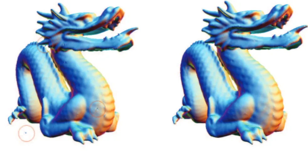
Figure 2. Dragon model: (left) result of the MPU algorithm which corresponds to our method for parameterslmax= 30,µ= 0.0,µ1= 1.0,
²= 0.0005andκ= 0.0. (right) result for parameterslmax= 30,µ= 0.01,µ1= 1.0,²= 0.0005andκ= 0.001: small artifacts are removed
0.001,0.0005,0.0002and for these values we were able to remove this small connected component and some of these artifacts, for κ = 0.0001 a small spurious com-ponent appear on the reconstructed surface. The use of ridge regression is necessary to remove the artifacts and the connected component a combination of (MPU + gra-dient one fitting) is not enough to get a good result.
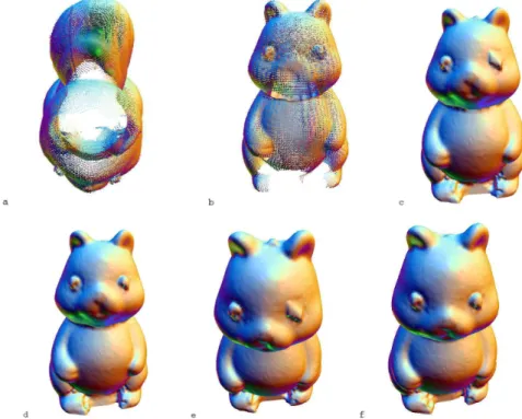
The effect of gradient one fitting is illustrated on the squirrel model (Figure 5), with incomplete point cloud, similarly to the usual output of laser scanner: the whole bottom part and details of the eyes and on the top are miss-ing. Subfigures c and e show the results of the only MPU method. Observe that, due to the big hole on the head, the MPU alone generated a bump and also inaccuracy on the right eye. The combination of the MPU with gradient one fitting (Subfigures d and f) is able to reconstruct the model without bump on the head and has a greater accuracy on the eyes. In this example the use of the ridge regression does not significantly alter the results with gradient one fitting. In general, the use of the gradient one fitting can be useful in the presence of small holes since it uses the neighboring normals.
7. CONCLUSIONS AND FUTURE WORKS
We proposed a new method that combines two power-ful techniques: theweighted gradient one fitting+ridge regression and themultilevel partition of unity. On one side, theridge regressionmethod has been considered by the pattern analysis community as one that gives a bet-ter fitting, since it tries to have a correct topology on the surface reconstruction. However, when the surface has a complex shape it is necessary to elevate the degree of the algebraic surface to get a good result. On the other side, themultilevel partition of unityis an implicit method
that is now one of the most important reconstruction tech-niques. In order to compute local approximations, it uses a complicate objective function. Thus, our surface recon-struction scheme not only takes the advantage of these two well recognized methods, but also unifies those meth-ods in a simple setting.
We plan to continue this work in several directions: one possible direction is to determine an approximated tangent planeTto the samples on the node of the tree and over this plane we consider the surface as a height field and determine a bivariate local approximationQ(x, y) :
T →R. Also overT we can consider better
approxima-tions like for example using wavelets method in order to be able to faithfully reproduce the oscillations and details (texture) on each region.
Figure 3. Knot model, with parameterslmax= 30,µ= 0.01,
Figure 5. Squirrel model. Figures a) and b) show the Squirrel point cloud, notice the holes on the top and the front, also there are small holes in the eyes. Pictures c) show the results of the MPU methodlmax= 20,µ= 0.0,µ1= 1.0and²= 0.005and picture d) shows the conbination of the
MPU and gradient one fitting with parameters (lmax= 20,µ= 0.01,µ1= 1.0and²= 0.005) respectivetly. Pictures e) and f) show the results of
pictures c) and d) from some inclination angle
Figure 4. Armadillo model, with parameters werelmax= 25,
µ= 0.01,µ1= 1.0,²= 0.0005andκ= 0.0.
ACKNOWLEDGMENTS
This work was partly supported by the Brazilian Min-istry of Science and Technology (MCT/CNPq Univer-sal 02/2006), and the State of Rio de Janeiro (FAPERJ Primeiros projetos 2004).
REFERENCES
[1] I. Babuska and J. Melenk. The partition of unity method. International Journal of Numerical Meth-ods in Engineering, 40:727–758, 1997.
[2] M. M. Blane, Z. Lei, H. Çivi, and D. Cooper. The 3L algorithm for fitting implicit polynomial curves and surfaces to data. Transactions on Pattern Analalysis and Machine Intelligence, 22(3):298–313, 2000.
[3] Y.-L. Chen and S.-H. Lai. A partition-of-unity based algorithm for implicit surface reconstruction using belief propagation. In Shape Modeling and Appli-cations, pages 147–155. IEEE, 2007.
[5] J. P. Gois, V. Polizelli, T. Etiene, E. Tejada, A. Castelo, T. Ertl, and L. G. Nonato. Robust and adaptive surface reconstruction using partition of unity implicits. InSibgrapi, pages 95–104. IEEE, 2007.
[6] M. Levoy, K. Pulli, B. Curless, S. Rusinkiewicz, D. Koller, L. Pereira, M. Ginzton, S. Anderson, J. Davis, J. Ginsberg, J. Shade, and D. Fulk. The digital Michelangelo project: 3D scanning of large statues. InSiggraph, pages 131–144. ACM, 2000.
[7] G. Taubin. Estimation of planar curves, surfaces, and nonplanar space curves defined by implicit equations with applications to edge and range image segmentation. Pattern Analysis and Machine Intel-ligence, 13(11):1115–1138, 1991.
[8] J. Carr, R. Beatson, J. Cherrie, T. J. Mitchell, W. R. Fright, B. C. McCallum, and T. R. Evans. Re-construction and representation of 3D objects with radial basis functions. In Siggraph, pages 67–76. ACM, 2001.
[9] T. Lewiner, H. Lopes, A. W. Vieira, and G. Tavares. Efficient implementation of Marching Cubes’ cases with topological guarantees. Journal of Graphics Tools, 8(2):1–15, 2003.
[10] M. Alexa, J. Behr, D. Cohen–Or, S. Fleishman, D. Levin, and C. Silva. Point set surfaces. In Vi-sualization, pages 21–28. IEEE, 2001.
[11] M. Alexa, J. Behr, D. Cohen–Or, S. Fleishman, D. Levin, and C. Silva. Computing and rendering point set surfaces.Transactions on Visualization and Computer Graphics, 9(1):3–15, 2003.
[12] T. K. Dey and S. Goswami. Provable surface re-construction from noisy samples. Computational Geometry: Theory and Applications, 35(1–2):124– 141, 2006.
[13] N. Amenta and M. Bern. Surface reconstruction by voronoi filtering. Discrete and Computational Ge-ometry, 22(4):481–504, 1999.
[14] N. Amenta, S. Choi, T. Dey, and N. Leekha. A sim-ple algorithm for homeomorphic surface reconstruc-tion. In Symposium on Computational Geometry, pages 213–222. ACM, 2000.
[15] N. Amenta, S. Choi, and R. Kolluri. The Power Crust, unions of balls, and the medial axis trans-form. Computational Geometry: Theory and Ap-plications, 19(2-3):127–153, 2001.
[16] Y. Ohtake, A. Belyaev, and M. Alexa. Sparse low-degree implicit surfaces with applications to high quality rendering, feature extraction, and smooth-ing. In Symposium on Geometry processing, page 149. Eurographics, 2005.
[17] Y. Ohtake, A. Belyaev, M. Alexa, G. Turk, and H.-P. Seidel. Multi-level partition of unity implicits. In
Siggraph, volume 22, pages 463–470. ACM, 2003.
[18] T. Tasdizen, J. P. Tarel, and D. B. Cooper. Alge-braic curves that work better. In Computer Vision and Pattern Recognition, volume II, pages 35–41. IEEE, 1999.
[19] M. Lage, F. Petronetto, A. Paiva, H. Lopes, T. Lewiner, and G. Tavares. Vector field reconstruc-tion from sparse samples. InSibgrapi, pages 297– 304. IEEE, 2006.
[20] D. Levin. Mesh-independent surface interpolation, pages 37–49. Springer, 2003.
[21] B. Mederos, N. Amenta, L. Velho, and L. de Figueiredo. Surface reconstruction for noisy point clouds. In Symposium on Geometry Processing, pages 53–62, 2005.
[22] V. V. Savchenko, A. Pasko, O. Okunev, and T. Kuni. Function representation of solid reconstructed from scattered surface points and contours. Computer Graphics Forum, 14:181–188, 2002.
[23] A. Sharf, T. Lewiner, G. Shklarski, S. Toledo, and D. Cohen-Or. Interactive topology–aware surface reconstruction. InSiggraph, pages 43.1–43.9, 2007.
[24] I. Tobor, P. Reuter, and C. Schlick. Reconstruct-ing multi-scale variational partition of unity im-plicit surfaces with attributes. Graphical Models, 68(1):25–41, 2006.