1.Empresa Brasileira de Aeronáutica – São José dos Campos/SP – Brazil. 2.Departamento de Ciência e Tecnologia Aeroespacial – Instituto Tecnológico de Aeronáutica – Divisão de Engenharia Aeronáutica e Mecânica – São José dos Campos/SP – Brazil.
Correspondence author: Henrique Gazzetta Junior | Avenida Cassiano Ricardo, 1.411 – Apto. 84B | CEP: 12.240-540 – São José dos Campos/SP – Brazil | E-mail: henrique.gazzetta@gmail.com
Received: May 17, 2016 | Accepted: Jul. 10, 2017 Section Editor:Dimitrios Pavlou
ABSTRACT: This article describes the run time characteristics of a gas turbine performance simulation using different solvers and components off-design performance database formats. Two different nonlinear systems of equation solvers, Newton-Raphson’s and Broyden’s, and two different formats of compressor and turbine off-design performance database (maps), tabulated values and fi tted surface equations, were compared. Based on the results it is then possible to trade off and select the most appropriate combination of solver and component map type for the gas turbine performance simulation for real-time application.
KEYWORDS: Propulsion, Gas turbines, Aircraft engines, Performance, Computer simulation.
INTRODUCTION
Th e simulation activities have been more used in the industry in earlier phases of the aircraft design. It is due to the recognition of value in identifying potential issues or even exploring the systems characteristics in early phases of the design. Th e necessary corrections or modifi cations obtained by the simulation results are far less costly to be implemented in earlier design phases, when there are no manufactured parts or signed contracts with suppliers, in comparison with the changes required in later phases, when changes in real parts or even in already closed interfaces may be required. Th e knowledge of the aircraft engine performance and transient characteristics is important to support optimization studies when the aircraft and the engine are still open for modifi cations. A gas turbine performance prediction tool is key in this process. A high-fi delity real-time engine transient performance calculation tool could support steady state and transient engineering analysis, system integration studies or even enable tests with pilot in the loop in earlier phases of the aircraft development. Th erefore, a real-time gas turbine performance code was specially developed to attend those necessities. Th is article aims to compare the simulation time using two diff erent nonlinear systems of equation solver methods: Newton-Raphson’s and Broyden’s. Th ese two methods were implemented into the developed computer program in order to verify which one gives the best performance for real-time application.
Run time Assessment for Gas Turbine
Performance Simulation
Henrique Gazzetta Junior1, Cleverson Bringhenti2, João Roberto Barbosa2, Jesuíno Takashi Tomita2
Gazzetta Junior H, Bringhenti C, Barbosa JR, Tomita JT (2018) Run time Assessment for Gas Turbine Performance Simulation. J Aerosp Tecnol Manag, 10: e1418. doi: 10.5028/jatm.v10.692 How to cite
Gazzetta Junior H https://orcid.org/0000-0001-9454-476X
Bringhenti C https://orcid.org/0000-0001-7634-1352
Barbosa JR https://orcid.org/0000-0001-8912-6045
METHODOLOGY
MODEL DESCRIPTIONA brand new engine simulation model was developed to simulate gas turbine performance in real time. The model has the ability to use different solvers and different compressor and turbine maps types. In addition to the engine thermodynamic cycle parameters, the model consider also the run time. In this work, a two-shaft direct drive gas turbine was chosen to be studied. The engine architecture is shown in Fig. 1 following the proposed nomenclature from SAE AS755 (2004). The computational code was developed in a modular structure, each module representing an engine component with its own characteristics, and then linked to each other to get the whole engine performance. This type of structure gives to the program flexibility to simulate several engine configurations without changing the program structure. The components modeling and other model features are described in more details in Gazzetta (2017) and Gazzetta et al. (2017). The model simulation main process diagram is shown in Fig. 2.
Figure 1. Two-shaft direct drive turbofan engine model diagram. AMB Air I
n
let
Fa
n
Fan air valve
HP Customer bleed LPT blade cooling HTP blade cooling HTP NGV cooling LPT NGV cooling
Fan bleed C om pr es sor HPC AMB AMB LPShaft HPShaft Pow
er E xt rac tio n A ft erb ur n er Je t pip e T urb in e HPT T urb in e LPT B ur n er B o os
ter 3 4 5
0 1 2 13 25 45 15 16 9
6 61 7
HPTP w rX WB15 M ix er Sp li ter 12 23 18 P o w er E xt rac tio n LPTP w rX
Bypass duct 17
E xha us t N o zzle 8 E xha us t N o zzle WB3 WC3 D WC3 C WC3 A WC3 B
Figure 2. Engine simulation process diagram.
DESIGN POINT
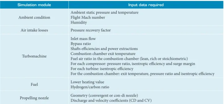
At design point, a full characterization of the ambient condition, air intake losses, turbomachine, fuel and propelling nozzles are required for the thermodynamic cycle calculation. Typical data required for that are shown in Table 1.
Design Point (DP) Off-Disign Point (ODP)
DP input read ODP input read
DP simulation First guess for interative process
Components map reading ODP Simulation
Components map scaling
Simulation converged? Output the simulation results
and scaled maps
02/13
Simulation module Input data required
Ambient condition
Ambient static pressure and temperature Flight Mach number
Humidity
Air intake losses Pressure recovery factor
Turbomachine
Inlet mass flow Bypass ratio
Shafts efficiencies and power extractions Combustion chamber exit temperature
Fuel air ratio in the combustion chamber (lean, rich or stoichiometric) For each compressor: pressure ratio, isentropic efficiency and surge margin For each turbine: isentropic efficiency
For the combustion chamber: exit temperature, pressure ratio and isentropic efficiency
Fuel Lower heating value
Hydrogen/carbon ratio
Propelling nozzle Geometry (convergent or con-di nozzle)
Discharge and velocity coefficients (CD and CV) Table 1. Required input for design point run.
All those information are used to set the design condition and scale the component maps for off-design simulations. At off-design conditions, only the ambient condition and one single power setting parameter are required as input data for the thermodynamic cycle calculation. All the air intake, turbomachine and propelling nozzles characterization are defined by off-design characteristics mapped in tables and maps. As a power setting it may be used burner exit temperature, shaft speed, fuel flow or thrust. An iterative procedure is used to set the turbomachine operation to match the input power set. The iterative procedure is described in the off-design section.
Additional information regarding the main engine components mathematical model, used to calculate the engine performance parameters, is described in Gazzetta (2017) and Gazzetta et al. (2017); for more details the reader can consult the literature (McKinney 1967; Koenig and Fishback 1972; Fishback 1972; Szuk 1974; Palmer and Cheng-Zhong 1974;
Macmillan 1974; Sellers 1975; Wittenberg 1976; Flack 1990; Stamatis et al. 1989; Ismail and Bhinder 1991; Korakianitis
and Wilson 1994; Baig and Saravanamuttoo 1997; Bringhenti 1999; Bringhenti 2003; Saravanamuttoo et al. 2001, Walsh and
Fletcher 2004).
OFF-DESIGN
For the two shaft engine architecture chosen to be studied in this paper the nonlinear system of equation is composed by six equations and six variables (Equations: LP shaft work balance; LP shaft mass flow balance; HP shaft work balance; HP shaft mass flow balance; engine core mass flow balance and fuel flow/max cycle temperature constraint. Variables: Engine mass flow; fan pressure ratio; HP compressor pressure ratio; HP turbine pressure ratio; LP turbine pressure ratio and fuel flow). The equations are described in Eqs. 1-6.
Nozzle vs. inlet mass flow balance (Conservation of mass):
where: W2 is the core inlet mass flow; W8 is the core nozzle mass flow; WB23 is the bleed air from booster; WB3 is the bleed air from high pressure compressor and WF is the engine fuel flow.
Low-pressure shaft power balance (Conservation of energy):
where: PwrFAN is the power required by the fan; PwrBooster is the power required by the booster; PwrLPT is the power produced by the low-pressure turbine; HPXLP is the shaft power extracted from the LP shaft and ηLPShaft is the low-pressure shaft mechanical efficiency.
High-pressure shaft power balance (Conservation of energy):
where: PwrHPCis the power required by the high-pressure compressor; PwrHPT is the power produced by the high-pressure turbine; HPXHP is the shaft power extracted from the HP shaft and ηHPShaft is the high-pressure shaft mechanical efficiency.
Power setting constraint: one of the following constraints will be selected based on the user input. The user can run the off-design simulation to match fuel flow, net thrust, burner exit temperature and shaft speeds:
where: WF is the engine calculated fuel flow; WFTgt is the engine target fuel flow; FN is the engine calculated net thrust; FNTgt is the engine target net thrust; T4 is the burner calculated exit temperature; T4Tgt is the burner target temperature; N1 and N2 are the calculated low- and high-pressure shaft speeds respectively; N1Tgt and N2Tgt are the low and high-pressure target shafts speeds respectively.
High-pressure turbine mass flow balance (Conservation of mass):
where WHPT is the calculated high-pressure turbine mass flow and W4 is the burner exit mass flow. Low-pressure turbine mass flow balance (Conservation of mass):
where: WLPT is the calculated low-pressure turbine mass flow and W4 is the burner exit mass flow.
(2)
(3)
(4)
(5)
In order to find the most appropriate nonlinear system of equations solver for the gas turbine performance simulation two different methods were tested: Newton-Raphson and Broyden.
Newton–Raphson’s method is widely know and used to solve nonlinear system of equations. It is based on the idea of linear approximation to calculate the next iteration steps:
where: f is the function whose zeros are being searched; x is the free variable; JFis the Jacobian calculated for the system of equations; F is a matrix with the solution of each equation calculated for x
k
Broyden’s method (Broyden 1965) is a generalization of the secant method to nonlinear systems. The secant method replaces the Newton’s method derivative by a finite difference:
where: f is the function whose zeros are being searched; x is the free variable; k is the iteration number. Broyden gave a system of equation generalization:
where: JF is the Jacobian calculated for the system of equations; F is a matrix with the solution of each equation calculated for xk; x is the free variable; k is the iteration number.
Thus, it is not necessary to calculate the Jacobian and all its derivatives of the Newton’s method, therefore this method is time-saving at a cost of lower convergence rate.
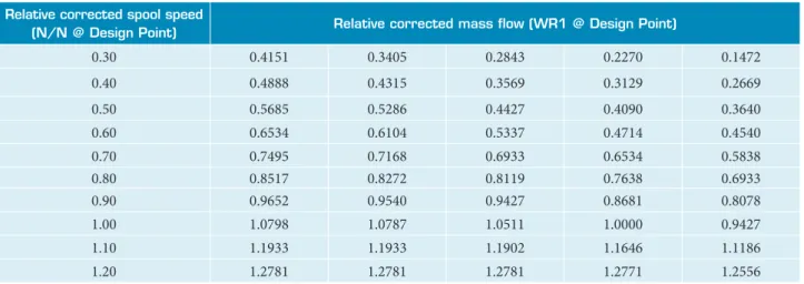
It was also compared two different types of compressor and turbine map data: tabulated and fitted surface equation. The tabulated map format is very well known and widely used by all gas turbine performance simulation tools. In this format, the map data is organized in a table format and the simulation shall interpolate the tables to find the off-design operating condition. The format of the tabulated map is shown in Tables 2, 3 and 4. Map data was obtained from Bringhenti (1999).
In order to completely avoid the interpolation task in the maps it is proposed to use surfaces equations instead of tables to represent the component off-design characteristics. The 3D surface equations are generated from the original tabulated map data and shall be representative of the points in the table. The expression derived to represent the maps and their general format is
where: x, y and f (x,y) represent any combination of parameters that better matches the tabulated data in the component map and N is the equation order. The parameters Ci,jin Eq. 12 are calculated based on the least squares methodology applied for polynomials of degree N as in Miller (2006), Dai et al. (2007) and Chernov and Ma (2011). This format of surface equation was chosen because the polynomial equations can be fitted in scattered data by using least squares methodology and because it gives flexibility in the (7)
(9) (8)
(10)
(11)
trade between fitting accuracy and equation complexity simply by changing the order of the equation. It was selected ninth order for this assessment due to better fitting to the map data.
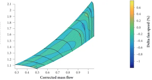
For the fitted surface equation, it was chosen to calculate compressor or turbine speed given pressure ratio and corrected mass flow. This methodology provides a very good matching between the tabulated data and calculated by the fitting surface equation, as shown in Figs. 3 and 4.
Table 2. Relative corrected mass flow tabulated map.
Table 4. Isentropic efficiency tabulated map. Table 3. Pressure ratio tabulated map. Relative corrected spool speed
(N/N @ Design Point) Relative corrected mass flow (WR1 @ Design Point)
0.30 0.4151 0.3405 0.2843 0.2270 0.1472
0.40 0.4888 0.4315 0.3569 0.3129 0.2669
0.50 0.5685 0.5286 0.4427 0.4090 0.3640
0.60 0.6534 0.6104 0.5337 0.4714 0.4540
0.70 0.7495 0.7168 0.6933 0.6534 0.5838
0.80 0.8517 0.8272 0.8119 0.7638 0.6933
0.90 0.9652 0.9540 0.9427 0.8681 0.8078
1.00 1.0798 1.0787 1.0511 1.0000 0.9427
1.10 1.1933 1.1933 1.1902 1.1646 1.1186
1.20 1.2781 1.2781 1.2781 1.2771 1.2556
Relative corrected spool speed
(N/N @ Design Point) Compressor pressure ratio
0.30 1.000 1.0420 1.0576 1.0672 1.0720
0.40 1.000 1.0600 1.1128 1.1380 1.1500
0.50 1.000 1.0760 1.1740 1.1980 1.2220
0.60 1.000 1.1320 1.2400 1.2844 1.2980
0.70 1.000 1.2220 1.2760 1.3360 1.4008
0.80 1.000 1.3000 1.3420 1.4296 1.4980
0.90 1.000 1.3288 1.3900 1.5424 1.6000
1.00 1.000 1.3312 1.5100 1.6420 1.7200
1.10 1.000 1.4860 1.6720 1.8004 1.8760
1.20 1.000 1.4680 1.7200 1.8700 1.9900
Relative corrected spool speed
(N/N @ Design Point) Compressor pressure ratio
0.30 0.7559 0.7665 0.7559 0.7251 0.6415
0.40 0.7559 0.7920 0.8026 0.7762 0.7401
0.50 0.7506 0.8026 0.8439 0.8281 0.7762
0.60 0.7454 0.8281 0.8800 0.8281 0.8078
0.70 0.7251 0.8545 0.8800 0.9011 0.8272
0.80 0.6882 0.8545 0.8800 0.9011 0.8272
0.90 0.6415 0.8281 0.8589 0.8800 0.8175
1.00 0.6002 0.7762 0.8589 0.8589 0.7867
1.10 0.5694 0.7762 0.8078 0.7762 0.7251
"
7060
50
40
30
20
10
0
–1.0 –0.8 –1.6 –0.4 –0.2 0.0 0.2 0.4 0.6 0.8 1.0 Delta to tabulated data (%)
Fr
eq
u
en
cy
Average
Standard Deviation
2.1
2
1.9
1.8
1.7
1.6
1.5
1.4
1.3
1.2
1.1
0.3
Corrected mass flow
P
ress
ur
e r
at
io
D
el
ta f
an s
p
ee
d (%)
0.4 0.5 0.6 0.7 0.8 0.9 1
–1 –0.8 –0.6 0.6
–0.4 0.4
–0.2 0.2
0.0
Figure 3 shows the delta between fan speed calculated by the fitted surface and the tabulated data. Only the tabulated map knots were considered in the comparison, with no interpolation. The maximum and standard deviation around 0.4% and 0.1% respectively, in addition to the average centered in 0%, mean that the chosen surface equation is a good representation of the tabulated data.
Figure 4 shows the same comparison of the Fig. 3 identifying where in the fan map the differences are located. The importance of this chart is to show that there are no high deviation spots that could affect the off-design calculation.
In order to test the convergence time, the model was run at different off-design conditions to explore different component map regions. The off-design conditions were set by inputting different altitudes, Mach numbers, temperatures and one engine power set, burner exit temperature in this assessment. The same set of data in the same sequence was used in the two solver methods and map types. Table 5 summarizes the chosen values used to simulate different engine operational conditions and Table 6 the combinations of solvers and map types.
Figure 3. Histogram of fan speed delta between tabulated map data and calculated by the fitted surface equation at same pressure ratio and corrected mass flow.
Table 5. Simulation test matrix.
Simulation key inputs Input values range
Altitude From sea level up to 15,000 m in steps of 500 m
Mach number From static up to 0.8 in steps of 0.05
Delta from standard day From –30 °C up to +30 °C in step of 5 °C
Burner exit temperature From 1800 K down to 1000 K in steps of 100 K
Name Solver Map type
Tab-NRaphson Newton-Raphson Tabulated
Tab-Broyden Broyden Tabulated
EQ-NRaphson Newton-Raphson Equation
EQ-Broyden Broyden Equation
Table 6. Combinations of solvers and map types.
RESULTS
The run time distribution and the number of iterations until the convergence are shown, for each combination of solver and map type as per Table 6, in the histogram charts below. The run times were achieved in a personal computer with Intel Core i7 920 at 2.67GHz and the solver convergence criteria was set to square root of the machine precision which was, in the computer where the points were run, 10-8.
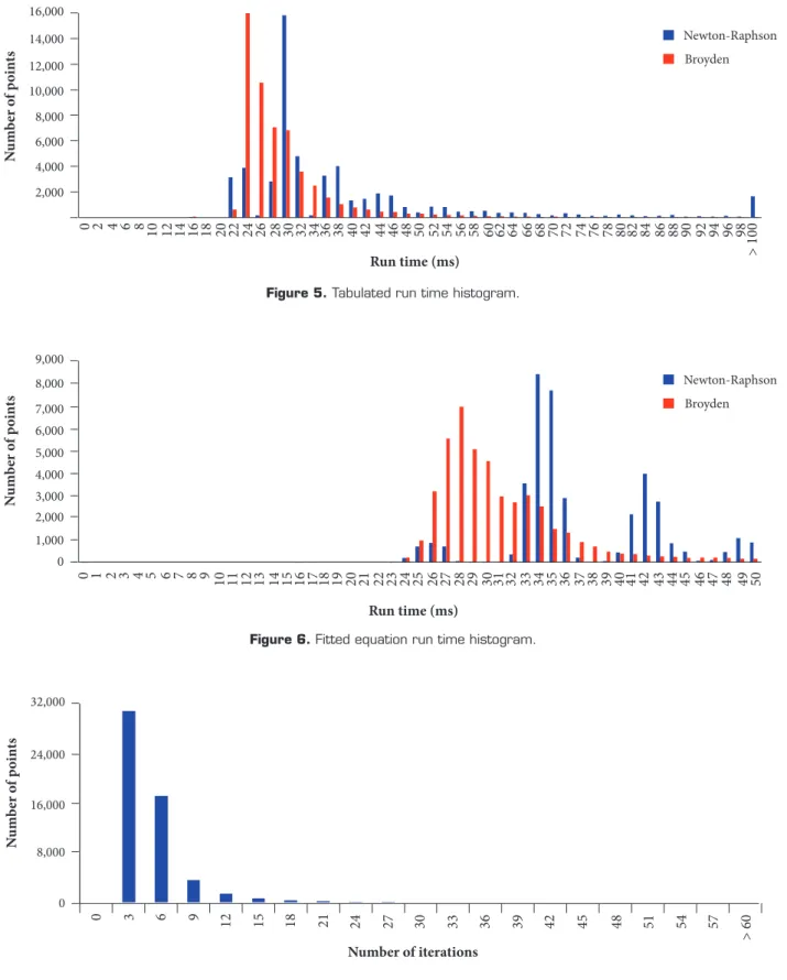
The simulation run times for the cases specified in Table 5 are shown in Figs. 5 and 6. The results are disposed in histogram charts where it is shown the distribution of the number of converged points, in the ordinates, by the elapsed time until convergence, in abscissas. The points and the operating conditions evaluated are described in Table 5.
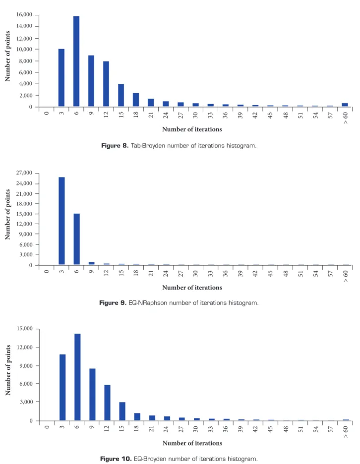
Similar charts are used to show the distribution of the number of iterations until the convergence. From Fig. 7 to Fig. 10, the histograms charts show the distribution of the number of converged points, in ordinates, by the number of iterations until the convergence, in the abscissas.
The histogram charts from Fig. 7 to Fig. 10 show that Broyden’s method generally takes more iterations than Newton-Raphson’s to reach the solution but takes shorter clock time. It is because Newton-Raphson’s method performs the derivatives calculation several times to build the Jacobian, which is very time-consuming, while Broyden’s method calculates the Jacobian just once in the first iteration. Another conclusion is that the fitted surface equations, defined from tabulated maps after fitting methods, are more computationally costly than the tabulated map due to the high order of the equations to keep a good matching with the tabulated data. In this study, it was used fitting surface equation of ninth order.
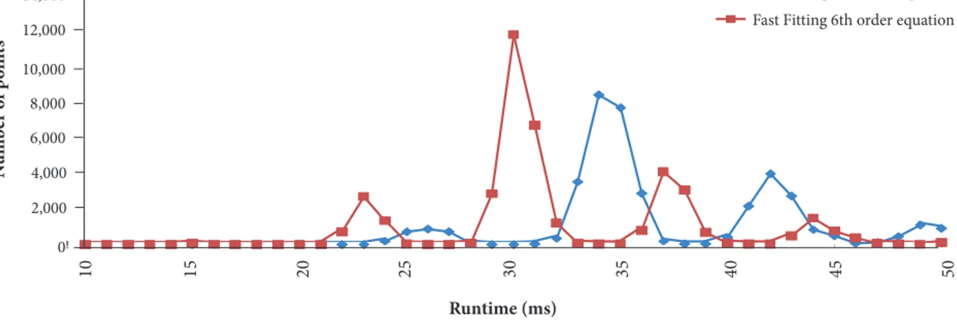
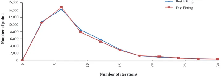
By reducing the order of the map, fitting surface equation to sixth instead of ninth order the simulation time was improved for both solvers while the number of iteration to reach the solution remains the same as shown in Figs. 11 to 14. It means that the solver is doing the same iterations but spending less time on each one due to lower number of surface equation terms. Reduced order of the fitting surface equation may lead to lower fidelity at off-design simulation.
Figures 11 and 12 are histograms that show distribution of the number of converged points, in ordinates, by the run time in the abscissas. The peaks offset to the left in both Newton-Raphson’s and Broyden’s methods show that most of the points spent less clock time to reach the solution when the fitted surface equations were simpler (6th order instead of 9th).
2,000
N
um
b
er o
f p
o
in
ts
4,000 6,000 8,000 10,000 12,000 14,000 16,000
Newton-Raphson
Broyden
Run time (ms)
0 2 4 6 8 10 12 14 16 18 20 22 24 26 28 30 32 34 36 38 40 42 44 46 48 50 52 54 56 58 60 62 64 66 68 70 72 74 76 78 80 82 84 86 88 90 92 94 96 98
> 100
2,000
1,000 0
N
um
b
er o
f p
o
in
ts
3,000 4,000 5,000 6,000 7,000 8,000 9,000
Newton-Raphson
Broyden
Run time (ms)
0 1 2 3 4 5 6 7 8 9 10 11 12 13 14 15 16 17 18 19 20 21 22 23 24 25 26 27 28 29 30 31 32 33 34 35 36 37 38 39 40 41 42 43 44 45 46 47 48 49 50 Figure 5. Tabulated run time histogram.
Figure 6. Fitted equation run time histogram.
8,000
0
N
um
b
er o
f p
o
in
ts
16,000 24,000 32,000
Number of iterations
0 3 6 9 12 15 18 21
24 27 30 33 36 39 42 45 48 51 54 57
> 60
9,000
3,000 6,000
0
N
um
b
er o
f p
o
in
ts
15,000
12,000 21,000
18,000 27,000
24,000
Number of iterations
0 3 6 9 12 15 18 21
24 27 30 33 36 39 42 45 48 51 54 57
> 60
6,000
3,000
0
N
um
b
er o
f p
o
in
ts
9,000 12,000 15,000
Number of iterations
0 3 6 9
12 15 18 21 24 27 30 33 36 39 42 45 48 51 54 57
> 60
4,000
2,000
0
N
um
b
er o
f p
o
in
ts
8,000
6,000 12,000
10,000 16,000
14,000
Number of iterations
0 3 6 9
12 15 18 21 24 27 30 33 36 39 42 45 48 51 54 57
> 60
Figure 9. EQ-NRaphson number of iterations histogram.
! 6,000
4,000
2,000
0
N
um
b
er o
f p
o
in
ts
8,000 12,000
10,000
14,000 Best Fitting 9th order equation
Fast Fitting 6th order equation
Runtime (ms)
10 15 20 25 30 35 40 45 50
Figure 11. Maps surface equation order impact in run time for EQ-NRaphson.
4,000 3,000
2,000 1,000
0
N
um
b
er o
f p
o
in
ts
5,000 6,000 8,000 7,000
9,000 Best Fitting 9th order equation
Fast Fitting 6th order equation
Runtime (ms)
10 15 20 25 30 35 40 45 50
15,000
10,000
5,000
0
N
um
b
er o
f p
o
in
ts
20,000 25,000
30,000 Best Fitting
Fast Fitting
Number of iterations
0 5 10 15 20 25 30
Figure 12. Maps surface equation order impact in run time for EQ-Broyden.
CONCLUSIONS
A brand new engine performance prediction model was built with the ability to use two different nonlinear system of equations solvers, Newton-Raphson’s and Broyden’s, and two different component map format, tabulated and fitted surface equation. Using the simulation results, all possible combinations of solvers and maps format were compared in terms of run time and number of iterations until the solution, including an additional map fitted surface equation option with a reduced equation order. Several different computational tools were found to fit polynomial surface equations in a scattered data; however, none of them was capable to fit high order equations, necessary to not degrade the map calculation accuracy. Therefore, a new tool was developed based on the existing least squares methodology expanded to high order surface equation to generate the maps equations.
Among the options tested and compared in this paper, the conclusion is that the most appropriate solver for a real-time gas turbine performance simulation is the Broyden’s method combined with the tabulated map. An additional comparison with a lower order map fitted surface equation shows that, if high fidelity model is not extremely required or if the run time is more important than the model accuracy (in flight simulator, for instance), the map fitted surface equation could be considered combined with Broyden’s method.
ACKNOWLEDGEMENTS
The financial support from Empresa Brasileira de Aeronáutica (Embraer), Conselho Nacional de Desenvolvimento Científico e Tecnológico (CNPq), Centro de Pesquisa e Inovação Sueco-Brasileiro (CISB), and Svenska Aeroplan AB (SAAB) is acknowledged.
AUTHOR’S CONTRIBUTION
Conceptualization, Gazzetta Junior H, Bringhenti C, Barbosa JR and Tomita JT; Methodology, Gazzetta Junior H, Bringhenti C and Barbosa JR; Investigation, Gazzetta Junior H; Writing – Original Draft, Gazzetta Junior H; Writing – Review & Editing, Gazzetta Junior H; Supervision, Bringhenti C and Barbosa JR.
10,000
8,000
6,000
4,000
2,000
0
N
um
b
er o
f p
o
in
ts
12,000 14,000
16,000 Best Fitting
Fast Fitting
Number of iterations
0 5 10 15 20 25 30
REFERENCES
Baig MF, Saravanamuttoo HIH (1997) Off-design performance prediction of single-spool turbojets using gasdynamics. J Propulsion 13(6). doi: 10.2514/2.5240
Bringhenti C (1999) Análise de desempenho de turbinas a gás em regime permanente (MsC thesis). São José dos Campos: Instituto Tecnológico de Aeronáutica. In Portuguese.
Bringhenti C (2003) Variable geometry gas turbine performance analysis (PhD thesis). São José dos Campos: Instituto Tecnológico de Aeronáutica.
Broyden CG (1965) A class of methods for solving nonlinear simultaneous equations. Math Comp 19:577-593. doi: 10.2307/2003941
Chernov N, Ma H (2011) Least Squares fitting of quadratic curves and surfaces (PhD thesis). Birmingham: University of Alabama.
Dai M, Newman TS, Cao C (2007) Least-Squares-based fitting of paraboloids, Department of computer science. Pattern Recognition 40:504-515. doi: 10.1016/j.patcog.2006.01.016
Fishback LH, Koenig RW (1972) GENENG 2: A program for calculating design and off-design performance of two- and three-spool turbofans with as many as three nozzles. Washington, DC: NASA (NASA TN D-6553). doi: 10.1016/0010-4485(73)90223-6
Flack RD (1990) Analysis and matching of gas turbine components. International Journal of Turbo and Jet Engines 7:217-226.
Gazzetta Jr H (2017) Real-time gas turbine generic model for performance evaluations. (PhD thesis). São José dos Campos: Instituto Tecnológico de Aeronáutica.
Gazzetta Jr H, Bringhenti C, Barbosa JR, Tomita JT (2017) Real-time gas turbine model for performance simulations. Journal of Aerospace Technology and Management Vol.9, No3, 346-356. doi: 10.5028/jatm.v9i3.693.
Ismail IH, Bhinder FS (1991) Simulation of aircraft gas turbine engines. Journal of Engineering for Gas Turbines and Power 113:95. doi: 10.1115/90-gt-342
Koenig RW, Fishback LH (1972) GENENG: A program for calculating design and off-design performance for turbojet and turbofan engines. Washington DC: NASA (NASA TN D-6552).
Korakianitis T, Wilson DG (1994) Models for predicting the performance of Brayton-Cycle engines. Journal of Engineering for Gas turbines and Power 116:381. doi: 10.1115/92-gt-361
Macmillan WL (1974) Development of a modular type computer program for the calculation of gas turbine off design performance. Cranfield: Cranfield Institute of Technology.
McKinney JS (1967) Simulation of Turbofan Engine – SMOTE: Description of Method and Balancing Technique. Ohio: Air Force Aero Propulsion Lab. pt.1-2 (AD-825197/AFAPL-TR-67-125).
Miller SJ (2006) The method of least squares. Providence, USA: Mathematics Department Brown University.
Palmer JR, Cheng-Zhong Y (1974) TURBOTRANS: A programming language for the performance simulation of arbitrary gas turbine engines with arbitrary control systems. [S.1.:s.n.] (ASME Paper 82-GT-200). doi: 10.1515/tjj.1985.2.1.19
SAE International (2004) SAE AS755 aircraft propulsion system performance station designation and nomenclature revision D, SAE Aerospace.
Saravanamuttoo HIH, Rogers GFC, Cohen H (2001) Gas turbine theory. 5th ed. Pearson Education.
Sellers J. Daniele C (1975) DYNGEN: A program for calculating steady-state and transient performance of turbojet and turbofan engines. Washington, DC: NASA (NASA TN D-7901).
Stamatis A, Mathioudakis K, Papailiou KD (1989) Adaptive simulation of gas turbine performance. Volume 1: Turbomachinery. doi: 10.1115/89-gt-205
Szuk JR (1974) HYDES: A generalized hybrid computer program for studying turbojet or turbofan engine dynamics. Washington, DC: NASA (NASA TM X-3014).
Walsh PP, Fletcher P (2004) Gas turbine performance. 2nd ed. Oxford: Blackwell Science.

