PVT EXPERIMENTAL AND MODELLING STUDY OF SOME SHALE RESERVOIR FLUIDS FROM ARGENTINA

(1)

of Chemical

Engineering

ISSN 0104-6632 Printed in Brazil www.scielo.br/bjce

Vol. 35, No. 02, pp. 313 - 326, April - June, 2018 dx.doi.org/10.1590/0104-6632.20180352s20160321

PVT EXPERIMENTAL AND MODELLING STUDY

OF SOME SHALE RESERVOIR FLUIDS FROM

ARGENTINA

#

Martin Cismondi

1,*

_{, Natalia G. Tassin}

1

_{, Carlos Canel}

2

_{, Francisco}

Rabasedas

2

_{and Carlos Gilardone}

2

1 _{Instituto de Investigación y Desarrollo en Ingeniería de Procesos y Química Aplicada} (IPQA), Universidad Nacional de Córdoba – CONICET. Córdoba, Argentina. 2_{Field Development Consultants (FDC de Argentina SRL). Buenos Aires, Argentina.}

(Submitted: May 19, 2016; Revised: January 9, 2017; Accepted: January 19, 2017)

Abstract - Shale reservoir fluids have been receiving much attention, especially during the last decade, due to the important reserves confirmed in many places around the world and the recent production growth in the United States, Argentina, and probably other countries to follow. In some fields of the Vaca Muerta formation in Argentina, the fluids can be classified as gas condensate or near-critical in some cases, presenting retrograde condensation of up to 30% in volume. This work presents compositional and PVT data of two gas condensate fluids, together with a new methodology for assigning molecular weights and densities to the different carbon number fractions when measured values are available for the whole fluid or liquid phase and only a weight fraction is collected through chromatography for each single cut. A thermodynamic modelling study of these fluids, and also a third one classified as volatile oil, is based on both the PR (Peng and Robinson, 1976) and RKPR (Redlich Kwong Peng Robinson, apud Cismondi and Mollerup, 2005) equations of state, together with different ways of characterizing the heavy fractions. The focus is on phase envelopes, but knowing only the saturation point at the reservoir temperature, and also on retrograde behavior.

Keywords: Gas Condensate, RKPR EoS, Phase Envelope, Retrograde Condensation, Characterization.

INTRODUCTION

Since 2005, and in the context of an important decline in the reserves of conventional hydrocarbon resources, Argentina has been facing the challen-ge of maintaining the production level of gas, the

main component of its energy matrix. The difference

between the demand and production curves should be

compensated by fluids from new non-conventional re -servoirs, mainly Shale Gas.

In many of the recently discovered fields, the pro

-duced fluids could be classified as near-critical, wi -th some cases presenting retrograde condensation of around 30% in volume at the reservoir temperature.

(2)

Material balances and numerical simulations, which

are used for predicting the fluids production beha

-vior and proposing development strategies, require an adequate characterization of the reservoir fluids and a good fitting of the laboratory data, in order to adequa

-tely reproduce field and well behaviors.

As far as we know, and despite the relevance of the Vaca Muerta formation, no articles have been pu-blished so far containing PVT or compositional data

on the produced fluids. A Scopus search for the words

“Vaca Muerta” by the end of year 2016 returned 24 publications, starting from 2003, all of them related to geological studies of the formation. A second search with the words “Shale” + “Argentina” returned 10 pu-blications, again with focus mainly on geological as-pects, and including also two articles published in the Journal of Petroleum Technology, on trends and pers-pectives about the production of shale gás and shale

oil worlwide (Beckwith, 2011). But no specific data on the fluids could be found.

This work presents compositional and PVT data obtained at the ITBA-FDC laboratory for two gas

con-densate fluids from different fields corresponding to

the Vaca Muerta formation in Argentina. The experi-mental methods are summarized in the next section. Then, a new methodology for assigning molecular

weights and densities to the different carbon number fractions is described and implemented to the two flui -ds and also a third one from the FDC data base, which

was classified as volatile oil. Finally, another section is

dedicated to a thermodynamic modeling study of the

fluids, based on two different cubic equations of sta

-te: the PR EoS (Peng and Robinson, 1976) and RKPR EoS (Redlich Kwong Peng Robinson, apud Cismondi and Mollerup, 2005), and exploring the effects of di

-fferent factors on the equation-of-state description of the fluids, including different ways of representing the

heavy residual fraction.

EXPERIMENTAL METHODS AND EQUIPMENT

The compositional analysis and PVT tests perfor-med at the ITBA-FDC laboratory followed essentially the procedures described in the books by Danesh (1998) and Pedersen and Christensen (2006), for the case of surface separator samples. Chromatographic analyses were carried out according to the norms

ASTM D-1945/03, GPA 2286 and ISO 6976/95 for gases, and EPA 8015 and ASTM D-2789 for liquid chromatography. The main equipment involved, for the fluids reported in this work, were the following:

(a) PVT cell “DBR-Jefri”, serial 0150-100-200,

maximum pressure: 10000 psi, maximum tempera-ture: 200 ºC; (b) chromatograph HP6890 G1530A with a capillary column HP-PONA Methyl Siloxane HP 19091S-001; (c) chromatograph HP6890 G1530A with a capillary column HP-PONA Methyl Siloxane HP 19091S-001 and a packed column DC200-PO-TM – HP 19006 80005. With both chromatographs the car-rier was hydrogen, with a FID front detector and TCD back detector.

The reservoir fluid tested in the PVT cell is the re

-sult of the recombination of a gas sample and a liquid

sample taken from the separator at the surface of the well, according to the gas-oil ratio (GOR), which is

also obtained from the flows measured at the surfa

-ce separator. Sin-ce the liquid sample is taken at the separator pressure, it also needs to be flashed before

analyzing its composition. Then, the steps leading to

the analytical determination of the reservoir fluid com -position are the following:

• Determination of the separator gas composition by chromatography.

• Determination of the separator liquid composition

through the following procedure:

▪ A flash separation of the liquid sample is per -formed at atmospheric pressure and room tem-perature, obtaining the so called flash gas and

flash liquid.

▪ The volumes of the two recovered phases are measured and the gas-liquid ratio is obtained. ▪ The compositions of the flash gas and liquid

phases are determined by chomatography.

▪ The average molecular weight for the flash li

-quid is determined by the melting point depres -sion method, using benzene as solvent.

▪ The flash liquid density is measured using a

pycnometer and a high precision weighing scale.

▪ The separator liquid composition is determi -ned from a recombination of the flash gas and

liquid compositions, in a similar way to what

is described, for example, in section 2.2 of the book by Pedersen and Christensen (2006).

• Finally, the reservoir fluid composition is determi -ned from the recombination of the separator gas

and liquid phases.

Tables 1 and 2 present the compositions of two

different gas condensate fluids analyzed at the

(3)

assigned according to the methodology described in

the next section. The five pseudo-components at the

end of each Table correspond to the decomposition of the residual C20+ fraction. More details are given in

the next section and specifically in Table 6.

Table 1: Composition for the Gas Condensate fluid

identified as GC1 in this work

Component Molar

Fraction

Molecular Weight

Density (g/cm3₎

Nitrogen 0.01744 28.01

Carbon Dioxide 0.00042 44.01

Methane 0.75731 16.04

Ethane 0.08026 30.07

Propane 0.03625 44.09

iso-Butane 0.00652 58.12

n-Butane 0.01372 58.12

iso-Pentane 0.00516 72.15

n-Pentane 0.00596 72.15

C6 0.00877 84.00 0.685

C7 0.01263 96.63 0.710

C8 0.01255 109.27 0.732

C9 0.00739 121.90 0.753

C10 0.00592 134.53 0.771

C11 0.00426 147.16 0.788

C12 0.00361 159.80 0.803

C13 0.00321 172.43 0.817

C14 0.00275 185.06 0.829

C15 0.00247 197.69 0.840

C16 0.00198 210.33 0.851

C17 0.00184 222.96 0.860

C18 0.00139 235.59 0.868

C19 0.00126 248.22 0.876

C20+ 0.00694 328.44 0.907

Pseudo-component 1 0.00200 266.64 0.885

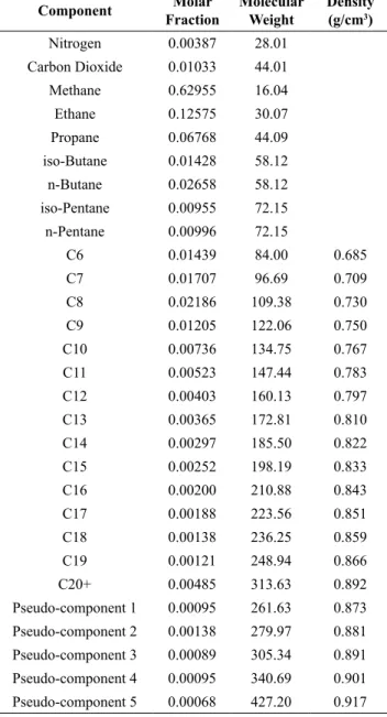
Table 2: Composition for the Gas Condensate fluid

identified as GC2 in this work

Fraction

Nitrogen 0.00387 28.01

Methane 0.62955 16.04

Ethane 0.12575 30.07

Propane 0.06768 44.09

iso-Butane 0.01428 58.12

n-Butane 0.02658 58.12

n-Pentane 0.00996 72.15

C6 0.01439 84.00 0.685

C7 0.01707 96.69 0.709

C8 0.02186 109.38 0.730

C9 0.01205 122.06 0.750

C10 0.00736 134.75 0.767

C11 0.00523 147.44 0.783

C12 0.00403 160.13 0.797

C13 0.00365 172.81 0.810

C14 0.00297 185.50 0.822

C15 0.00252 198.19 0.833

C16 0.00200 210.88 0.843

C17 0.00188 223.56 0.851

C18 0.00138 236.25 0.859

C19 0.00121 248.94 0.866

C20+ 0.00485 313.63 0.892

In order to study the PVT behavior of each

re-servoir fluid, a Constant Mass Experiment (CME) is

performed. This experiment is also referred to as a Constant Composition Expansion (CCE) or simply as

a Pressure-Volume (PV) test. Irrespective of the fluid

type, it is common practice to carry out a CME test at the reservoir temperature. This study consists of suc-cessive expansions of the PVT cell to reproduce the

evolution of the fluid at the reservoir temperature. In

this evolution, the dew point pressure and the amount

of retrograde liquid deposited in the cell at pressures

below the dew point are determined. The methodology is as follows:

• A physical recombination from the separator samples is charged to a Robinson PVT cell. This double-window cell allows a direct observation

of the fluid and measurement of the volume of condensed liquid. The cell is kept at the reservoir temperature and the fluid is pressurized through a

hydraulic piston.

• The monophasic condition of the sample is

veri-fied. A visual confirmation is enough for gas con

-densate fluids, while an additional verification of the compressibility through a differential pressure

(4)

• The total volume is registered at different pres -sures, measuring also the volume of retrograde

liquid accumulated at pressures below the dew

point, which is determined visually.

• The curves pressure vs. relative volume, as well as

% of retrograde liquid vs. pressure are determined.

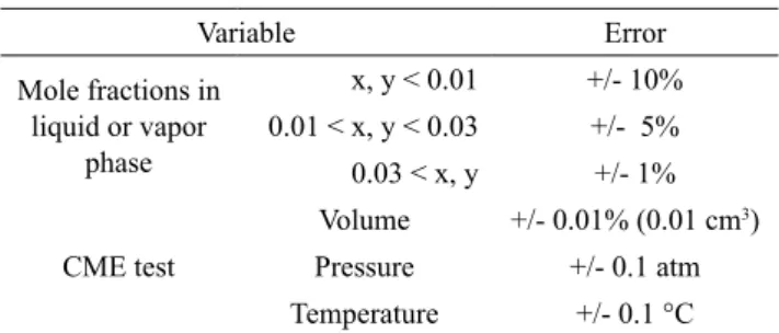
Regarding experimental uncertainties in the PVT

tests, it is difficult to estimate a level of accuracy for the different values informed, since several stages are involved and different factors can affect the results.

Nevertheless, based on the repeatibility experience accumulated at the ITBA-FDC lab, the assumed com-positional errors are given in Table 3, together with

uncertainties for the different measurements associa -ted with the CME test.

(1978), whose table is also included in books covering

these topics, like the one by Pedersen and Christensen (2006, see Table 2.1 in the book) .

Those values may work quite well in many cases,

providing reasonable values for the residual fraction, e.g., C20+, but may also lead to unreasonable estima-tions for the residual fracestima-tions when the real values of densities or molecular weights for the SCN fractions

have important differences with the assumed genera -lized values. In the latter case, a consistent characte-rization of the residual fraction (typically C20+) will

be clearly hindered, since solving the equations that equal average values with measured density or mole

-cular weight for the whole fluid makes it accumulate

the errors in the previous SCN fractions, for which it will have to compensate.

Therefore, in this work we propose a new methodo-logy for the estimation of molecular weights and den-sities for single carbon cuts from C6 on, based on

me-asured values for the fluid and general assumptions on

the distribution or evolution of these properties along

SCN fractions in reservoir fluids.

It is a well established fact that the diversity of mole-cular structures within a given SCN fraction increases with carbon number. For example, most C6 fractions consist mainly of n-hexane, plus some cyclopentane

and different quantities of a few branched hexanes. On

the other hand, as it is illustrated for example in Table 2.4 in the book of Pedersen and Christensen (2006), a C9 fraction already includes typically more than 20

different compounds detected by chromatography, including normal and branched paraffinic, naphthe -nic and aromatic structures. For fractions around C20

there can be various dozens of different compounds, with very small quantities of each, and it could be very difficult to achieve a complete list for a specific fluid. As a consequence of that, there is normally no risk in

assuming typical values for the density and molecular

weight of C6, while the differences can be important

for higher cuts. For that reason, we adopt the

recom-mended values from Katz and Firoozabadi only for C6, and assume specific mathematical functionalities

in terms of carbon number for the rest, depending on only one parameter for each property, which can be adjusted in order to match the measured value for the

whole fluid.

For molecular weights a linear relation with car-bon number is normally accepted. In our methodolo-gy, following the reasoning above, the corresponding

equation for estimating the SCN molecular weights is:

M_i = 84 + C(i − 6) (1)

Table 3: Experimental uncertainties associated with

the mole fractions determined for defined compounds

and measurements in the CME test.

Variable Error

Mole fractions in

liquid or vapor

phase

x, y < 0.01 +/- 10%

0.01 < x, y < 0.03 +/- 5%

0.03 < x, y +/- 1%

CME test

Volume +/- 0.01% (0.01 cm3₎

Pressure +/- 0.1 atm

Temperature +/- 0.1 °C

A new methodology for assigning molecular weights and densities

In some compositional studies of reservoir fluids

(see for example Pedersen et al., 1992) average mole-cular weights are calculated from the chromatographic single-component distributions for the C6-C9 frac-tions, and measured by freezing point depression for the distillate fractions obtained for higher cuts through True Boiling Point (TBP) analysis.

Nevertheless, in routine PVT studies like the ones reported here, it is more common that only a mass fraction can be assigned to each cut from C6 on,

ba-sed on measured quantities. Density at standard con -ditions and molecular weight are measured only for

each separator phase, and sometimes also for the C7+

or C10+ fractions.

Then, reported values for single carbon number (SCN) fractions are either estimated based on correla-tions, or taken from Tables of recommended generali-zed values. This has been a common practice in the in-dustry and a popular and typical source for generalized density and molecular weight values for single carbon

(5)

where i is a number identifying a SCN fraction and C

is an adjustable constant.

The relation with density is not that simple. Pedersen, for example, recommends a linear relation with the logarithm of the carbon number. Instead, in

this work, we use the following equation with A_d and

B_d being adjustable constants:

ρi = Ad * e

−i/10₊_B

d (2)

For this relation we have found a better correlation capacity when considering experimental values,

in-cluding those recommended by Katz and Firoozabadi (1978).

Fixing this equation to the typical recommended

value for C6, there is only one degree of freedom left, which can be associated with the A_d parameter, since

B_d becomes

B_d = 0.685 − A_d * e−0.6 (3)

Finally, as it is well established that there exist a high linearity between the logarithm of molar frac-tions and the carbon number of the corresponding cut

(Pedersen et al., 1992), the following equation will be

adopted for the distribution of the C20+ fraction:

ln(z_i) = A * i + B (4)

So, Eqs. (1-4) are our working equations, and the

proposed procedure for decomposing the available

mass fractions and assigning densities for the different

SCN fractions is as follows:

1) Find the value of C for Eq. (1) that leads to a

consistent distribution of fractions, where an ex-trapolation to the C20+ range is in agreement with

the measured values for the fluid. This requires

the following sub-steps:

a. Obtain the value of z₆₊ and products (z*M)i ba-sed on the experimental information available. b. For a given value of C, calculate the values of

the M_i’s (i= 6 to 19) from Eq. (1), and the cor -responding mole fractions as z_i = (z*M)_i / M_i. c. Calculate z₂₀₊ = z₆₊ − ∑_i₌₆z_i

d. Calculate M₂₀₊ = (z * M)₂₀₊ / z₂₀₊

e. Obtain the Best Feasible Extrapolation (Ramello and Cismondi, 2016) based on mole fractions from step b, providing the coefficients

A and B for the distribution (Eq. 4), and find

the corresponding Cmax where the summation reaches z₂₀₊.

19

f. Based on the estimated distribution of the C20+ fraction from the previous point, obtain the corresponding M₂₀₊= ∑_i₌₂₀z_i * M_i/z₂₀₊. If it

is not equal to the value from step d, estimate

a new value for C, e.g., following the secant method, and go back to step b.

2) Find the value of A_d for Eq. (2) that leads to re

-covering the density of the fluid. This requires the

following sub-steps:

a. Obtain the experimental value of V₆₊ (see Nomenclature section), depending on the in-formation available. With a report with densi-ty values assigned somehow, it is calculated as

V₆₊ = ∑_i₌₆ + . The following steps aim at a sort of redistribution of the densities (or volumes), considering that arbitrary values,

e.g. those from Katz and Firoozabadi (1978),

will be replaced by a continuous function like

Eq. (2) which, when applied from C6 to Cmax,

can consistently recover the density measured for the fluid.

b. For a given value of A_d, obtain the correspon-ding B_d from Eq. (3) and calculate the values of

the ρ_i’s (i= 6 to Cmax) from Eq. (2).

c. Obtain V_6+,_calc = ∑_i₌₆ .

d. If it is not equal to the V₆₊, estimate a new va-lue for A_d, e.g., following the secant method, and go back to step b.

3) Lump the C20+ distribution into Nps pseudo--components having similar mass fractions or z*M products. In this work Nps = 5.

Note that the products (z*M)_i are available based

on measurements, from the equation:

(z * M)_i= m_i/n_total where n_total = m_total/M_total (5)

and total can refer to C6+, C10+ or the complete fluid,

etc., depending on available measurements.

The procedure has been explained for fluids analyzed up to C20+, but would be equally applicable

to cases with C30+ or C35+.

Regarding the concept of Best Feasible Extrapolation referred to in step 1d, its detailed ex-planation is part of a parallel article to be published

soon (Ramello and Cismondi, 2017). Nevertheless, it essentially implies that an extrapolation based on Eq.

(4) and pre-20 mole fraction values will be applied to the 20+ range as long as the slope falls in between the two feasibility limits alluded to in the following lines. If the slope is too pronounced, the distribution along

calc Cmax

19 z_i M_i z20+M20+

ρi ρ20+

Cmax zi Mi

(6)

carbon numbers will go up to infinity without ever re -aching z₂₀₊. In this case, the limiting slope for which the summation of mole fractions reaches z₂₀₊ at infinity

(in practice, a high carbon number) will be adopted. On the other hand, if the slope is too small very low and unrealistic Cmax values can be obtained. In these cases, a slope leading to a Cmax near 60 is adopted.

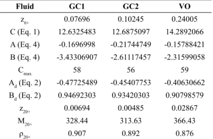
Table 4 presents the values of the different parame -ters involved for each of the analyzed gas condensate

fluids, and also a volatile oil from the FDC data base (VO in this work), whose composition and different

assigned values are given in Table 5. Details on the decomposition of the C20+ fractions, including car-bon numbers covered by each pseudo-compound and distribution of the z*M products, are given in Table 6.

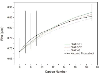
Figs. 1 and 2 show the molecular weight and den-sity functions obtained, in comparison to the

generali-zed values from Katz and Firoozabadi (1978) and also

some ranges of expected values. For fractions from C6 to C9 these ranges are given by the values corres-ponding to the single components that can be found, according to Table 2.4 in the book of Pedersen and Christensen (2006), while the ranges for C19 covers

the values found in more than 30 reservoir fluids taken

from the works of Pedersen et al. (1992), Jaubert et al. (2002) and also Chapter 3 in the book of Pedersen and Christensen (2006). In comparison to those ranges and generalized values, the trends resulting from our pro-posed methodology appear to be reasonable. The two gas condensates GC1 and GC2 show nearly the same line for molecular weights and similar curves for den-sities. The volatile oil presents the higher molecular weights and lower densities, which could be an

indica-tion of a more paraffinic fluid than the others.

Table 4: Parameters related to the proposed molecular weight and density functions, together with the

distribution of the C20+ fraction, for the three fluids

studied in this work.

Fluid GC1 GC2 VO

z₆₊ 0.07696 0.10245 0.24005

C (Eq. 1) 12.6325483 12.6875097 14.2892066

A (Eq. 4) -0.1696998 -0.21744749 -0.15788421

B (Eq. 4) -3.43306907 -2.61117457 -2.31599058

C_max 58 56 59

A_d (Eq. 2) -0.47725489 -0.45407753 -0.40630662

B_d (Eq. 2) 0.94692303 0.93420303 0.90798579

z₂₀₊ 0.00694 0.00485 0.02867

M₂₀₊ 328.44 313.63 366.43

ρ20+ 0.907 0.892 0.876

Table 5: Composition for the Volatile Oil identified

as VO in this work.

Fraction

Nitrogen 0.00525 28.01

Methane 0.51688 16.04

Ethane 0.10377 30.07

Propane 0.06374 44.09

iso-Butane 0.01214 58.12

n-Butane 0.03087 58.12

n-Pentane 0.01414 72.15

C6 0.02090 84.00 0.685

C7 0.03031 98.29 0.706

C8 0.03803 112.58 0.725

C9 0.02621 126.87 0.743

C10 0.01964 141.16 0.759

C11 0.01438 155.45 0.773

C12 0.01111 169.74 0.786

C13 0.01073 184.02 0.797

C14 0.00905 198.31 0.808

C15 0.00827 212.60 0.817

C16 0.00661 226.89 0.826

C17 0.00595 241.18 0.834

C18 0.00546 255.47 0.841

C19 0.00473 269.76 0.847

C20+ 0.02867 366.43 0.876

Table 6: Decomposition of the C20+ fraction from

each fluid into 5 pseudo-components.

Pseudo-component

GC1 GC2 VO

CN

range z*M

CN

range z*M

CN

range z*M

1 20-21 0.533 20 0.249 20-21 2.261

2 22-23 0.414 21-22 0.386 22-23 1.810

3 24-26 0.455 23-24 0.272 24-26 2.039

4 27-31 0.448 25-28 0.324 27-31 2.119

(7)

THERMODYNAMIC MODELLING

In this work we do not have the goal of achieving the best match or description of some behaviour for

the specific fluids studied. Instead, we rather want to use these cases in order to analyze how different as

-pects or parameters in the equation-of-state modelling of PVT properties may affect the results. Then, this

study is meant to provide some insight for future mo-delling works concerned with these types of reservoir

fluids, and probably help in guiding the definition of

new strategies for modelling algorithms.

Figure 1: Molecular weight values assigned to the reservoir fluids

according to the proposed methodology. Generalized values recommended

by Katz and Firoozabadi (1978) are included for comparison. Vertical bars

indicate ranges of expected values (see text).

Figure 2: Density values assigned to the reservoir fluids according to the

proposed methodology. Generalized values recommended by Katz and Firoozabadi (1978) are included for comparison. Vertical bars indicate

ranges of expected values (see text).

There are mainly three factors affecting the calcu

-lation of PVT properties, once an equation of state has been chosen to model a given reservoir fluid of known

composition, like the ones considered in this work: I) How to represent the residual heavy fraction, in

these cases C20+. Just as one pseudo-component? Decompose it? Into how many pseudo-compo-nents and how?

II) Critical temperatures and pressures (T_C, P_C), and also acentric factors, assigned to each pseudo--component from C6 on, typically as functions of density and molecular weight of each given frac-tion, and then eventually adjusted through some matching procedure.

III) Interaction parameters: typically the kij’s (attrac-tive ones) and alterna(attrac-tively lij’s (repulsive, not used in the common practice with classic models like PR).

In this study we defined and implemented three di

-fferent approaches in order to roughly see the effects

of choices regarding factors I and II:

Approach A: Fractions C6 to C19 are represented by n-alkanes with the same carbon numbers. The C20+ fraction is represented by another single n-alkane, the one with closest molecular weight.

Approach B: T_C and P_C for the pseudo-compo-nents representing fractions from C6 on are estimated by Pedersen correlations based on MW and density. The same for the acentric factor, using the correlation designed for PR. The C20+ is treated the same way, as if it were a single carbon number.

Approach C: Idem to Approach B, except that the

C20+ fraction is split into five pseudo-components wi

-th similar mass fractions. Details for -the fluids studied

here are provided in Table 6.

Note that Approach A, the simplest one, may be the least realistic among the three studied approaches. But it was considered in order to see –based on

compari-sons with Approach B- the effect of factor II on calcu -lations. Similarly, comparison between approaches B

and C will show the effects of decomposing the C20+

fraction (factor I).

In relation to factor III, we used approaches A to

C in two different ways: first a purely predictive mo -de, with default alkane-alkane interaction parameters taken from a previous work (Cismondi Duarte et al., 2015, adapted also to SCN cuts in approaches B and C as explained below). And then a matching mode,

whe-re a factor f affects all default interaction parameters

(both k_ij and l_ij for RKPR, k_ij for PR), and its value is

defined such that the experimental saturation pressure

(8)

Besides using estimated critical constants and acen-tric factors for any SCN fraction or pseudo-component in approaches B and C, their default parameters in the predictive mode were assigned according to the follo-wing rules:

- For the δ1 parameter (RKPR EoS) the following correlation defined by Cismondi Duarte et al.

(2015) for n-alkanes is adapted here for pseudo--components based on their molecular weights:

δ₁ = 0.91 + 0.33 * CNEff * e

(-CNEff

11

)

M − 2

14

; CNEff = (6)

- Interaction parameters k_ij (with methane and pro-pane) and l_ij (with all lighter defined alkanes) are

estimated using the same RKPR correlations pro -posed for n-alkanes by Cismondi Duarte et al. (2015), dependent on the a_c and δ₁ parameters of the components involved, respectively.

- All interaction parameters between pseudo-com-ponents are zero.

- For the PR EoS all l_ij interactions are zero, while

k_ij‘s with the lighter components are estimated ba-sed on correlations like the ones uba-sed by Cismondi

Duarte et al. (2015), but using an effective carbon

number, calculated as (M-2)/14, instead of the no-minal carbon number.

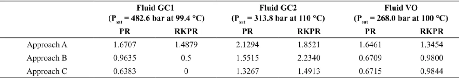
Table 7 presents the required values of f with the

different approaches and two models, for the three fluids considered. Only in two cases (Approaches B and C with RKPR for fluid GC1) was it not possible

to match the saturation pressure with a positive f va-lue. Therefore, f = 0.50 (giving the lowest error with Approach B) and f = 0 (null interaction parameters for Approach C, in order not to invert the sense of the de-fault values) were applied for making the comparisons. Figs. 3 to 8 show the predicted phase envelopes for

the three fluids, with both the pure predictive and the

matching mode. There is a clear trend showing that the

extent of predicted immiscibility, and consequently

also the predicted saturation pressure, increases from approach A to B and from B to C.

Table 7: Matching of saturation pressure: Multiplying factors f for interaction parameters of the PR and RKPR

equations of state, with the different fluids studied in this work.

Fluid GC1 (P_sat = 482.6 bar at 99.4 °C)

Fluid GC2 (P_sat = 313.8 bar at 110 °C)

Fluid VO (P_sat = 268.0 bar at 100 °C)

PR RKPR PR RKPR PR RKPR

Approach A 1.6707 1.4879 2.1294 1.8521 1.6461 1.3454

Approach B 0.9635 0.5 1.5515 2.2340 0.6709 0.9800

Approach C 0.6383 0 1.3267 1.4913 0.6715 0.9844

Figure 3: Pure predictions of the phase envelope for fluid GC1, with the

PR and RKPR equations of state and the three approaches considered.

Default interactions for alkanes assigned to all fractions.

Figure 4: Predictions of the phase envelope for fluid GC1 with the PR

and RKPR equations of state and the three approaches considered, when the f value in Table 7 multiplies all interactions in order to match the

(9)

Figure 5: Pure predictions of the phase envelope for fluid GC2, with the

PR and RKPR equations of state and the three approaches considered.

Default interactions for alkanes assigned to all fractions.

Figure 6: Predictions of the phase envelope for fluid GC2 with the PR

experimental saturation pressure at the reservoir temperature.

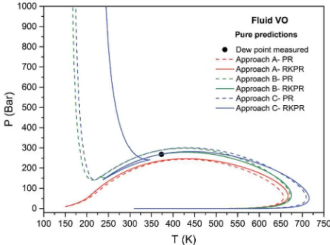
Figure 7: Pure predictions of the phase envelope for fluid VO, with the PR

and RKPR equations of state and the three approaches considered. Default

interactions for alkanes assigned to all fractions.

Figure 8: Predictions of the phase envelope for fluid VO with the PR

experimental saturation pressure at the reservoir temperature.

Accordingly, the f values in Table 7 show the oppo

-site evolution: Approach A always requires the highest

f values in order to match the experimental pressure,

while Approach C always requires values lower than

one, given the overestimation obtained from pure pre-dictions. Two partial exceptions can be observed: The

first one involves a very high f value for the GC2 fluid with RKPR and approach B, denoting a low sensitivi -ty of the envelope around the reservoir temperature, probably related to the combination of kij and lij inte-ractions. The second appears in the volatile oil (VO), where there is practically no change in the predicted

saturation pressure when going from approach B to C,

i.e., there is practically no effect from decomposing

the C20+ fraction in this regard.

It is important to remark that predictions

correspon-ding to Approaches B and C in Figs. 3, 5 and 7 should

not be considered as a demonstration of the predicti-ve potential of these approaches, since such potential could only be developed when appropriate interaction

(10)

weight and density of each fraction. Nevertheless, ap-proaches B and C have shown a reasonable predictive capacity for the saturation pressures available,

espe-cially with RKPR for the volatile oil.

Once again, we emphasize that the three

approa-ches implemented in this work were defined in order to study the effect of three different factors separately:

representation of the residual fraction, pure (pseudo-) component parameters and interaction parameters. Indeed, results in Figs. 3 to 8 show that all of them

play an important role in the fluids investigated, and that the effects are even more appreciable for the gas

condensates than for the volatile oil. Moreover, the

sa-me types of effects are observed either with the PR or the RKPR EoS.

A specific observation regarding the limitations of

Approach A can be made based on the results in Fig. 8. While the upper part of a gas condensate phase enve-lope can go either up or down in pressure as tempera-ture decreases, depending on the case (the divergence to higher pressures occurring for the most asymmetric

mixtures that show liquid-liquid like immiscibility), it most frequently goes down for a volatile or (espe -cially) black oil. This expected behaviour is indeed the one observed in Fig. 8 with approaches B and C, when the saturation pressure has been matched

throu-gh adjustment of the interaction coefficients (the on

-ly exception is given by approach B with RKPR, but liquid-liquid separation develops only up to tempera

-tures around 200 K). Nevertheless, the same procedu

-re leads to the artificial p-rediction of what could be a

wrong behaviour with approach A, apparently forced by the large values of interaction parameters that were

required to match the experimental saturation point. It

is interesting to see that this happens with both models,

even when they were parameterized very differently:

only constant kij values for the PR EoS (the classic way) and lij plus some temperature dependent kij for

the RKPR EoS (see Cismondi Duarte et al., 2015). It

should be noted that the crossings appearing in some

of the envelopes calculated with the RKPR EoS for the VO fluid denote three-phase behaviour, always below

the reservoir temperature, but we do not have evidence

to confirm or discard this possibility.

Other strong reasons for which it could be an

impor-tant mistake to represent the different SCN fractions as

n-alkanes are exposed in Fig. 9, which shows how the

M – ρ coordinates of real reservoir fluids are located at

important distances from the n-alkanes curve.

Figure 9: Data for reservoir fluids and their fractions, from three of the

main basins in Argentina (Canel and Mediavilla, 1990), in comparison to the n-alkanes molecular weight – density characteristic curve and the Cragoe Correlation (Craft and Hawkins, 1991). Points correspond to wells from the Vaca Muerta formation.

Figures 10 and 11 show the predicted liquid drop

--out curves for the GC1 and GC2 fluids, while the

corresponding pressure-volume curves are presented in Figs. 12 and 13. In all cases volume shift correla-tions were implemented. Predicted curves are shown in comparison to experimental data obtained from the CCE tests, as described before in the experimental section. Note that even when the reproduction of the saturation pressure is imposed on all approaches and models, the predicted retrograde behaviour below

su-ch common point can be very different from one case

to another (Figs. 10 and 11). The same observations

regarding the influence of all factors studied apply he -re, as for the prediction of phase envelopes. On the contrary, all pressure-relative volume curves look very

similar in Figs. 12 and 13. In the case of fluid GC2 (Fig. 13) curves seem to be affected only by the EoS

and not by the approach, with a better approximation

to the experimental curve by the RKPR EoS.

On the other hand, something that is specific to

the retrograde condensation curves and could not be

(11)

to Approach B with the same model. The effect is

perhaps clearer for GC2, with the B-C crossings at lower pressures, and also higher maximum values of condensation with Approach C, for which results are closer to the experimental. The same is valid for GC1

with PR and, in a way, also with RKPR except for the

shift in the curve for approach C, due to not matching the saturation pressure.

Figure 10: Predictions of the liquid drop-out curve for fluid GC1 at 372.55

K, with the PR and RKPR equations of state and the three approaches

considered. The f value in Table 7 multiplies all interactions in order

to match the experimental saturation pressure. Black dots represent measurements.

Figure 11: Predictions of the liquid drop-out curve for fluid GC2 at 383.15

K, with the PR and RKPR equations of state and the three approaches

considered. The f value in Table 7 multiplies all interactions in order

to match the experimental saturation pressure. Black dots represent measurements.

Figure 12: Predictions for the CCE Pressure-Volume curve for fluid

GC1 at 372.55 K, with the PR and RKPR equations of state and the three

approaches considered. The f value in Table 7 multiplies all interactions in

order to match the experimental saturation pressure. Black dots represent measurements

Figure 13: Predictions for the CCE Pressure-Volume curve for fluid

GC2 at 383.15 K, with the PR and RKPR equations of state and the three

approaches considered. The f value in Table 7 multiplies all interactions in

order to match the experimental saturation pressure. Black dots represent measurements.

This improvement would confirm the effect and ne -cessity of decomposing the C20+ fraction.

What was not expected are the correct shapes of the curves predicted with Approach A (only with the

RKPR EoS), even with a reasonable quantitative agre

-ement with the data for the GC1 fluid in Fig. 10. So far,

(12)

CONCLUSIONS

Compositional and PVT data have been reported

for two gas condensate fluids from the Vaca Muerta

formation in Argentina. Motivated by the fact that ea-ch composition was analyzed only by ea-chromatography, without making density and molecular weight measu-rements for each single fraction, a new methodology was developed to estimate these properties from C6 to C20+, based on selected functionalities with carbon

number and on measured values for the fluid. The pro

-posed strategy avoids use of the unique generalized values from Katz and Firoozabadi (1978) and would allow, instead, capturing the different characteristics of each fluid. It was applied to the two gas condensa

-tes, and also a third fluid classified as volatile oil.

A thermodynamic modelling study was carried out

for the three fluids, based on the PR and RKPR equa

-tions of state and three different approaches designed to evaluate the effects of different factors or degrees of

freedom involved in this type of modelling. In appro-ach A eappro-ach SCN fraction is treated as a normal alka-ne, while correlations based on density and molecular weight are used to estimate each fraction parameters in approaches B an C. Only in approach C a split of

the C20+ fraction into five pseudo-components is

performed.

Clear differences were found from the application of approaches A, B and C, and different observations were made that could help to define a more specific and complete methodology aiming at the quantitative description of the PVT behaviour of this type of fluids.

Both the phase envelopes and isothermal retrograde

condensation curves turned out to be quite sensitive to

the modelling approach, but not the CCE

pressure-re-lative volume curves. In particular, the best qualitative

representation of the experimental retrograde behavior in the CCE experiment for the gas condensates was obtained with approach C. This involves especially the higher pressure region, where the heaviest fractions

condense first, and would be a consequence of the mo -re detailed t-reatment of the C20+ fraction through 5

different pseudo-components. Much better quantita -tive results are expected for the near future if some

RKPR parameters are correlated with properties of the different fluid cuts, like density and molecular weight.

ACKNOWLEDGEMENTS

We want to thank Osvaldo Migliavacca for his work in the PVT lab.

We also acknowledge the financial support received

from the following Argentinean institutions: Consejo

Nacional de Investigaciones Científicas y Técnicas de

la República Argentina (CONICET), Agencia Nacional

de Promoción Científica y Tecnológica (ANPCyT),

and Universidad Nacional de Córdoba (UNC).

NOMENCLATURE

Abbreviations

CCE: Constant Composition Expansion.

CME: Constant Mass Experiment.

CN: Carbon Number.

EoS: Equation of State.

FDC: Field Development Consultants (FDC de Argentina SRL)

GC1: Gas Condensate fluid (N°1). GC2: Gas Condensate fluid (N°2). GOR: Gas-Oil Ratio.

HP: Hewlett-Packard

ITBA: Instituto Tecnológico de Buenos Aires

PR: Peng-Robinson equation of state. PV: Pressure-Volume.

PVT: Pressure, Volume and Temperature.

RKPR: Generalized

Redlich-Kwong-Peng-Robinson equation of state.

SCN: Single Carbon Number.

TBP: True Boiling Point.

VO: Volatile Oil fluid.

Roman letters

A: Constant in Eq. (4) for the estimation of

a SCN mole fraction.

A_d: Constant in Eq. (2) for the estimation of

a SCN fraction density.

B: Constant in Eq. (4) for the estimation of

a SCN mole fraction.

B_d: Constant in Eq. (2) for the estimation of

a SCN fraction density.

C: Constant in Eq. (1) for the estimation of

a SCN fraction molecular weight.

Ci (i=6 to 19): Hydrocarbon cut or fraction of the

reservoir fluid.

Ci+ (i=6, 7, 10, 20, 30 or 35): Residual fraction of

the reservoir fluid, containing the SCN

fractions starting from i and higher.

Cmax: For a given distribution of the C20+

(13)

f: factor involved in the matching mode.

i: number identifying a hydrocarbon SCN cut or fraction.

k_ij: attractive interaction parameter between compound “i” and compound “j”.

l_ij: repulsive interaction parameter between compound “i” and compound “j”.

M: Molecular weight.

m: Collected mass.

M₂₀₊: Molecular weight of the residual fraction C20+.

Nps: Number of pseudo-components.

P: Pressure.

T: Temperature.

V: Volume.

V₆₊: The volume occupied by the C6+

frac-tion per mole of total fluid. Since it is de

-fined just as an auxiliary variable in the

procedure of assigning density values for

the different SCN and residual fractions,

it refers to the same standard conditions

for which densities are defined.

z: Mole fraction.

z₆₊: Mole fraction of the residual fraction C6+.

z₂₀₊: Mole fraction of the residual fraction C20+.

Greek letters

ρ Density.

ρ₂₀₊ Density of the residual fraction C20+. Super/subscripts

c Critical property.

calc Calculated property.

i number identifying a hydrocarbon SCN cut or fraction.

sat saturation state.

REFERENCES

Beckwith, R., Shale Gas: Promising Prospects Worldwide. Journal of Petroleum Technology,

63(07), 37-40 (2011).

Beckwith, R., The trend toward shale oil. Journal of

Petroleum Technology, 63(7), 42-43 (2011).

Canel C. and Mediavilla J., Estudios PVT a partir de datos de boca de pozo. Proceedings of the 2das Jornadas de Informática Aplicada a la Producción. Argentina (1990).

Cismondi, M. and Mollerup, J., Development and

Application of a Three-Parameter RK-PR Equation

of State. Fluid Phase Equilibria, 232, 74-89 (2005).

Cismondi Duarte, M., Cruz Doblas, J., Gomez, M.J., Montoya, G.F., Modelling the phase behavior of alkane mixtures in wide ranges of conditions: New parameterization and predictive correlations

of binary interactions for the RKPR EOS. Fluid

Phase Equilibria, 403, 49-59 (2015).

Craft, B. C., and Hawkins, M., Applied Petroleum Reservoir Engineering, Prentice Hall PTR,

Englewood Cliffs, NJ 07632, 2nd_{ed. (1991).}

Danesh, Ali, PVT and Phase Behavior of Petroleum Reservoir Fluids, Elsevier (1998).

Jaubert, J-N, Avaullee, L. and Souvay, J-F. A crude oil data bank containing more than 5000 PVT and gas injection data. Journal of Petroleum Science and

Engineering 34, 65–107 (2002).

Katz, D.L. and Firoozabadi, A., Predicting phase

behavior of condensate/crude-oil systems using

methane interaction coefficients, J. Petroleum Technol. 20, 1649–1655 (1978).

Pedersen, K.S., Blilie, A.L., Meisingset, K.K., PVT calculations on petroleum reservoir fluids using

measured and estimated compositional data for the

plus fraction, Ind. Eng. Chem. Res. 31, 1378–1384

(1992).

Pedersen, K.S. and Christensen, P.L. , Phase Behavior

of Petroleum Reservoir Fluids, CRC/Taylor & Francis, Boca Raton (2006).

Peng, D.-Y., Robinson, D.B., A New Two-Constant

Equation of State, Industrial & Engineering Chemistry Fundamentals, 15, 59-64 (1976).