Paulo Flores Ribeiro • Luís Catela Nunes • Pedro Beja • Luís Reino • Joana Santana • Francisco Moreira • José Lima Santos
Paulo Flores Ribeiro (Corresponding author)
CEF – Centro de Estudos Florestais, Instituto Superior de Agronomia, Universidade de Lisboa. Tapada da Ajuda, 1349-017 Lisboa, Portugal
e-mail: [email protected]
phone: +351 213 653 325/ fax: +351 213 653 195
Luís Catela Nunes
Nova School of Business and Economics, Universidade Nova de Lisboa, Campus de Campolide, 1099-032 Lisboa, Portugal
e-mail: [email protected]
Pedro Beja
CIBIO/InBio, Centro de Investigação em Biodiversidade e Recursos Genéticos, Universidade do Porto. Campus Agrário de Vairão, Vairão, Portugal
CEABN/InBio, Centro de Ecologia Aplicada “Professor Baeta Neves”, Instituto Superior de Agronomia, Universidade de Lisboa, Tapada da Ajuda, 1349-017 Lisboa, Portugal
e-mail: [email protected]
Luís Reino
CIBIO/InBio, Centro de Investigação em Biodiversidade e Recursos Genéticos, Universidade do Porto. Campus Agrário de Vairão, Vairão, Portugal
CEABN/InBio, Centro de Ecologia Aplicada “Professor Baeta Neves”, Instituto Superior de Agronomia, Universidade de Lisboa, Tapada da Ajuda, 1349-017 Lisboa, Portugal
Universidade do Porto. Campus Agrário de Vairão, Vairão, Portugal
CEABN/InBio, Centro de Ecologia Aplicada “Professor Baeta Neves”, Instituto Superior de Agronomia, Universidade de Lisboa, Tapada da Ajuda, 1349-017 Lisboa, Portugal
e-mail: [email protected]
Francisco Moreira REN Biodiversity Chair
CIBIO/InBio, Centro de Investigação em Biodiversidade e Recursos Genéticos, Universidade do Porto. Campus Agrário de Vairão, Vairão, Portugal
CEABN/InBio, Centro de Ecologia Aplicada “Professor Baeta Neves”, Instituto Superior de Agronomia, Universidade de Lisboa, Tapada da Ajuda, 1349-017 Lisboa, Portugal
e-mail: [email protected]
José Lima Santos
CEF – Centro de Estudos Florestais, Instituto Superior de Agronomia, Universidade de Lisboa. Tapada da Ajuda, 1349-017 Lisboa, Portugal
1
A spatially explicit choice model to assess the impact of conservation
2policy on High Nature Value farming systems
3
4 Abstract
5 High Nature Value (HNV) farmland is declining in the EU, with negative consequences for
6 biodiversity conservation. Agri-environment schemes implemented under the Common
7 Agricultural Policy have addressed this problem, with recent proposals advocating direct
8 support to HNV farming systems. However, research is lacking on the economics of HNV
9 farming, which makes it difficult to set the level and type of support that ensure its
10 sustainability. In this paper, we focused on a Special Protection Area for steppe bird
11 conservation, analysing how economic incentives, biophysical and structural features
12 govern the choice of farming system. We found that persistence of the traditional farming
13 system important for steppe birds was associated with economic incentives, resistance to
14 change, and good quality soils, whereas a shift to specialised livestock production systems
15 was favoured by higher rainfall and less fragmented farms. A supply curve built using the
16 choice model predicted that the proportion of traditional farming increased from 20% to
17 80% of the landscape, when economic incentives increased from about 100€/ha to 160€ha.
18 Overall, our study highlights the dependence of HNV farming systems on economic
19 incentives, and provide a framework to assess the effects of alternative policy and market
20 scenarios to sustain farmland landscapes promoting biodiversity conservation.
21
22 Keywords: Discrete choice modelling; Common Agricultural Policy; Agri-environment
24
25 1. Introduction
26 The concept of High Nature Value (HNV) farmland was introduced in the early 1990s to
27 demonstrate the dependence of European biodiversity on traditional and low-input farming
28 systems (Beaufoy et al., 1994). Despite their importance, HNV farmland is declining due
29 to social, economic and policy pressures for either agricultural intensification or land
30 abandonment (Oppermann and Paracchini, 2012). This is compromising the objectives
31 established under the European Union (EU) Biodiversity Strategy to 2020 (European
32 Commission, 2011), and it reveals a failure of the Common Agricultural Policy (CAP) to
33 safeguard farmland biodiversity (Henle et al., 2008; Pe’er et al., 2014).
34 To improve the support for HNV farmland under the CAP, a recent report for the European
35 Commission suggested an approach based on payments to farms in HNV farmland or
36 operating HNV farming systems (Keenleyside et al. (2014a). There are, however, major
37 operational challenges related to lack of data or indicators to identify HNV farmland or
38 farming systems (Keenleyside et al., 2014a), as well as limited research on economic
39 aspects of HNV farming needed to establish the level and type of funding necessary for its
40 sustainability (Keenleyside et al., 2014a). Indeed, most studies carried out so far aimed at
41 estimating the costs for farmers to participate in agri-environment schemes (AES) (Oñate
42 et al., 2007; Bamière et al., 2011; Wätzold et al., 2015),or to assess farmer’s willingness to
43 accept a compensatory payment for management options benefiting the environment
44 (Buckley et al., 2012; Ruto and Garrod, 2009). These studies typically rely on survey data
45 from hypothetical choice experiment designs, or use models to estimate the costs of farm
46 management or land-use changes to comply with policy regulations. In both cases,
48 revealed preference approaches relying on observed ex-post behavioural data. Other recent
49 works advocate results-based payments, as an alternative to management-based schemes,
50 for farmland biodiversity conservation in HNV farmland (Keenleyside et al., 2014b).
51 However, the payment calculations are still based on the same principles set out in the EU
52 Regulations, which provide compensations for additional costs or income foregone
53 resulting from the commitments made, including a possible additional to cover for
54 transaction costs (Article 28(6) of Regulation (EU) No 1305/2013).
55 The potential of farming systems as a basis for developing agri-environment policy has
56 been suggested (Beaufoy and Marsden, 2011; Poux, 2013; Ribeiro et al., 2016a), supported
57 by studies evidencing links between farming systems and landscape features or farming
58 practices of conservation relevance (Bamière et al., 2011; Ribeiro et al., 2016a, 2016b).
59 This farming system approach represents a significant departure from current
agri-60 environment schemes, which are based on specific management requirements and imply
61 significant transaction costs (Mettepenningen et al., 2011; McCann, 2013; Pannell et al.,
62 2013). This approach could be implemented, for instance, using the concept of greening
63 the Pillar 1 of the CAP by granting a top-up payment to farmers operating farming systems
64 associated with HNV farmland in a specific region (Ribeiro et al., 2016a). This would
65 require identifying these HNV farming systems for different regions across the EU, and
66 calculating the payment level required to ensure sufficient uptake by farmers. Although the
67 underlying idea of an agri-environment policy aimed at supporting HNV farming systems
68 may sound interesting, however, the factors driving the farmer’s decision in choosing the
69 farming system are not well understood, nor is the role that economic incentives provided
70 by policies play in that decision.
71 Here, we developed a case study on a HNV farmland of extensive cereal-steppes in
73 conservation concern are associated with a traditional farming system involving rotational
74 cereal cultivation and sheep pasturing of fallows (Delgado and Moreira, 2000; Leitão et al.,
75 2010; Moreira, 1999; Moreira et al., 2012a, 2012b, 2007, 2004). In previous studies we
76 have demonstrated a strong dynamics of farming systems in this area in response to the
77 CAP reform of 2003 (Ribeiro et al., 2014), which may have affected landscape patterns
78 (Ribeiro et al., 2016b) and agricultural practices relevant for biodiversity conservation
79 (Ribeiro et al., 2016a). In this new study, we use the same setting to model the economic
80 rational of farming system changes, aiming at: 1) investigating the factors that influence
81 farmer’s choice of farming system, subject to biophysical, structural, policy and economic
82 drivers and constraints; and 2) developing a framework to simulate, on a spatially explicit
83 basis, the effects of different policy and market scenarios on HNV farmland. Results were
84 then used to evaluate the potential of our framework to outline empirical supply curves for
85 conservation services (Santos et al., 2008; Lewis and Wu, 2014), relating levels of
86 payment per hectare paid to farmers operating HNV farming systems with the amount of
87 farmland managed under such systems.
88 89
90 2. Methods
91 2.1. Study area
92 The study focused on an extensive HNV farmland area in the south of Portugal, covering
93 ca. 180,000 hectares (Fig. 1). The area is characterized by open fields, smooth relief, and
94 typical Mediterranean climate, with hot dry summers and moderately rainy cold winters. It
95 encompasses the Special Protection Area (SPA) of Castro Verde, classified under the EU
97 conservation concern. Studies carried out during the past 20 years suggest that
98 conservation of these steppe birds requires the maintenance of an extensive traditional
99 farming system based on rainfed cereal crops in rotation with long-term fallows grazed by
100 sheep, which dominated the landscape for decades (Moreira, 1999; Delgado and Moreira,
101 2000; Leitão et al., 2010; Reino et al., 2010; Moreira et al., 2012a, 2012b, 2007, 2004;
102 Santana et al., 2017, 2014). To support this traditional farming system, an AES is operating
103 since 1995, though with limited success for preventing land use changes (Ribeiro et al.,
104 2014) and protect bird diversity (Santana et al., 2014).
105
106
107 Fig.1. Location of the study area in southern Portugal, showing the farm-parcel structure and the Special
108 Protection Area (SPA) of Castro Verde where an agri-environment scheme (AES) is in operation since 1995.
109
110 Recent studies have shown a shift from the traditional to livestock-grazing specialized
111 farming systems in the area, despite de AES, possibly resulting from the decoupling of
113 decision to keep a direct payment on suckler cows, goats and sheep (Ribeiro et al., 2014).
114 These changes have affected landscape patterns (Ribeiro et al., 2016b) and agricultural
115 practices (Ribeiro et al., 2016a), but their effects on biodiversity are still poorly
116 understood. In at least some cases, however, changes are likely to be negative, including
117 for instance the anticipation of the cereals harvesting date under the livestock system,
118 which is judged to increase the destruction of bird nests (Ribeiro et al., 2016a). Another
119 problem may be the loss of the rich traditional landscape mosaic represented by cereal
120 fields, ploughed fields, and fallows of different ages and grazing intensity, which likely
121 reduces habitat diversity for birds (Oñate et al., 2007; Delgado and Moreira, 2000; Leitão
122 et al., 2010; Reino et al., 2010; Moreira et al., 2012a; Santana et al., 2017).
123
124 2.2. Farming systems identification
125 The dominant farming systems in the study area and their spatial dynamics during 2000
126 and 2010 were assessed by a cluster analysis performed on farm-level data from the EU
127 Integrated Administration and Control System (IACS), together with spatially explicit
128 farm-parcel data from the EU Land Parcel Identification System (LPIS). Such data has
129 been recommended for HNV farmland research (Beaufoy and Marsden, 2011; Beaufoy et
130 al., 2012; Keenleyside et al., 2014a), and it was successfully tested in previous studies
131 (Ribeiro et al., 2014, 2016b). Five farming systems were identified, including two
132 livestock specialized systems (the Cattle and Sheep systems), two systems specialized in
133 crop production (the Annual crops and the Permanent crops systems), and a mixed farming
134 system (the Traditional system) (details in Annex A in Supplementary Information). Due
135 to its land use pattern, dominated by a low-intensity cereal-fallow rotation, complemented
137 farming system underpinning the HNV of the study area. Each farm in each year was
138 assigned to one of these five farming systems, thereby providing information to assess
139 transitions over time.
140
141 2.3. Drivers and constraints of farming system choice
142 Each farm was characterised using biophysical (soil quality, terrain slope and average
143 annual rainfall) and structural features (farm size, farm spatial fragmentation and oak
144 woodlands) (details in Annex B of the Supplementary Information), expected to influence
145 farming system choice (Keenleyside et al., 2014b; Ribeiro et al., 2014). These variables
146 varied spatially but were largely constant over time within the study period.
147 To capture the effects of policy and market drivers on farmer decisions, we used the gross
148 income ratio to compare the economic profitability of the farming systems. This indicator
149 was used because there was no time-series on detailed farm-level production costs to
150 compute gross margins. We believe this is acceptable, since many of these farms have their
151 own means of production (workers and equipment), which are fixed costs largely
152 independent of the activities in which they are used, and not subject to significant
153 fluctuations during the 10-year time span of our study. Farm management decisions were
154 thus expected to be mostly driven by temporal variation in gross income from sales
155 revenues and direct subsidies. The gross income ratio for each farming system in each
156 study year t (𝐺𝐼𝑅𝑡) was defined as:
157 𝐺𝐼𝑅𝑡 = 𝐺𝐼𝑅𝐹𝑆𝑡 𝐺𝐼𝐴𝐹𝑆𝑡
158 where 𝐺𝐼𝑅𝐹𝑆𝑡 is the unit gross income of a reference farming system, and 𝐺𝐼𝐴𝐹𝑆𝑡 is the unit
160 Traditional farming system because it is the HNV system in our study area. If the
161 income/cost ratios of each activity do not vary significantly, then a higher GIR means a
162 higher relative profitability of the reference farming system. However, because different
163 productions may have very different gross income/cost ratios, we cannot interpret
164 𝐺𝐼𝑅𝑡= 1 as an indifference point between the reference and the alternative system.
165 To compute 𝐺𝐼𝑅𝑡, we first estimated the unit gross income of each farming system in each
166 study year (𝐺𝐼𝑡), in euros per hectare, as follows:
167 𝐺𝐼𝑡=
𝑛
∑
𝑖 = 1(
𝑄𝑖.𝐴𝑖.𝑃𝑡𝑖+ 𝐴𝑖. 𝑆𝑡 + 1𝑖)
168 where, for each activity i, Qi is the average regional yield per hectare (e.g. wheat,
169 sunflower, cattle, sheep), Ai is the area occupied (land shares), Pit is the producer price in
170 year t, and Sit+1 is the value of the direct subsidy in year t+1. We considered subsidies in
171 year t+1 because farmers normally make their annual production decisions with a
172 reasonable knowledge of the subsidies for the following year. Assuming that farmers make
173 their management decisions based on knowledge of local average yields, these were kept
174 constant during the study period. Decoupled CAP payments (e.g. the single payment
175 scheme) were not included to estimate 𝐺𝐼𝑡, because they do not depend on crop patterns
176 and thus are unlikely to influence directly the management decisions on productions. Data
177 on agricultural regional yields and producer prices were obtained from Portuguese official
178 statistics, and CAP direct payments were provided by the Portuguese CAP paying agency
179 (Table S4 in Annex C in Supplementary Information).
180 To capture the farmers’ perception on the recent trend in the relative profitability of the
181 farming systems, we use the change in GIRt over time, defined as GIRdif t = GIRt - GIRt-n,
183 upward trend in the profitability of the reference farming system, compared to alternative
184 systems, and vice versa.
185
186 2.4 Discrete choice model design
187 We used a discrete choice modelling approach based on logistic regression to investigate
188 the drivers of farming systems shifts. Logistic regression can assume the binomial or
189 multinomial form, depending on the number of farming systems specified as the
190 categorical dependent variable. The independent variables included the biophysical,
191 structural and policy constraints (Table S3 in Supplementary Information), and the
192 economic variables GIRt and GIRdif. A lagged dependent variable identifying the farming
193 system in the previous period (FSlag) was included to account for adjustment costs and
194 persistence effects considered by the farmer when making decisions.
195 To handle possible heterogeneity in farmers’ preferences due to uncontrolled variables
196 influencing motivations and attitudes towards policies, such as those describing
socio-197 cultural profiles (de Snoo et al., 2013; Siebert et al., 2006), we used latent class models to
198 account for heterogeneity in preferences (Greene, 2012). These models have been widely
199 used in recent stated-preference studies using discrete choice models, including within the
200 context of agri-environment policy evaluation (Garrod et al., 2012; Ruto and Garrod, 2009;
201 Villanueva et al., 2014). Since data included repeated observations on the same farms over
202 time, a panel data model was estimated, allowing for individual-specific heterogeneity in
203 preferences that are constant over time (Greene, 2012).
204 A stepwise-like procedure was used in model building, starting by estimating the model
205 with all candidate independent variables, and considering 1, 2 and 3 latent classes, and then
207 procedure was repeated until all variables were significant at the 5% level. To assess model
208 fit and decide on the number of latent classes for the optimal model, we used the Akaike
209 Information Criterion (AIC) and the Bayesian Information Criterion (BIC) (Boxall and
210 Adamowicz, 2002; Gruen and Leisch, 2008; Greene, 2012; Villanueva et al., 2014).
211 Prediction accuracy was assessed by fitting the model on a training subset containing 75%
212 of randomly selected observations, and then applying it on a test set with the remaining
213 25% observations.
214 All statistical analysis were performed using the R software, version 3.1.1 (R Development
215 Core Team, 2015). The latent class models were estimated using the “FlexMix” R package,
216 version 2 (Gruen and Leisch, 2008).
217
218 2.5. Assessment of policy and market scenarios
219 We used the choice model to assess the impacts of several policy and market scenarios on
220 farming systems. This was carried out by evaluating how changes in GIR would affect the
221 representation of different farming systems in the landscape. The approach was based on
222 the idea that GIR integrates changes in economic incentives such as the complete
223 decoupling of direct payments on suckler cows and sheep, changes in livestock market
224 prices resulting from the review of EU border taxes on beef products, or the
225 implementation of an AES paying a premium to HNV farming systems. Therefore,
226 farmer’s responses were assumed to respond to economic incentives inasmuch they affect
227 GIR, rather than considering the details of policy change.
228 To provide a measure of uncertainty in the simulation of scenarios, we use the approach to
229 calculate 95% confidence intervals based on Monte Carlo simulations (Krinsky and Robb,
231 normal distribution, using the estimated coefficients as the means vector and the
232 corresponding standard errors and covariances as the variance-covariance matrix. These
233 1000 model replicas were successively run over a pre-set range of GIR values simulating
234 the effects of any policy or market changes, using 2010 as a baseline, and observing the
235 corresponding impact on the proportion of the study area covered by the farming systems.
236 For each output simulation, we recorded the values corresponding to quantiles 0.025, 0.500
237 and 0.975 from the 1000 outcomes of the model, and the results were used to outline a
238 supply curve for biodiversity conservation services, expressed as a proportion of the area
239 covered by the Traditional system, bounded by a 95% confidence interval.
240 Simulations results were also used to assess the likely impact of policy and market
241 scenarios on biodiversity, considering that the SPA of Castro Verde was created primarily
242 to protect steppe bird assemblages (Ribeiro et al., 2014; Santana et al., 2014). Therefore,
243 we assessed how changes in farming systems would affect habitat suitability for steppe
244 birds, assuming that they are favoured by landscapes where livestock densities (in
245 livestock units per hectare - LU/ha) and the proportion of cereal area early harvested for
246 hay production (CEH) are low, and where the areas covered by the traditional farming
247 system (P_RFS), and the mean patch area (MPA) and number of patches (NPATCH) of
248 this farming system are large. Although these metrics provide an indirect link between
249 farming systems and the conservation of steppe bird species, they reflect ecological
250 information on these species collected in the study area during the last 20 years (Moreira,
251 1999; Delgado and Moreira, 2000; Leitão et al., 2010; Reino et al., 2010; Moreira et al.,
252 2012a, 2012b, 2007, 2004; Santana et al., 2017, 2014). Landscape metrics were computed
253 using the “SDMTools” R package, version 1.1-221 (Vanderwal et al., 2015).
255
256 3. Results
257 Significant farming systems dynamics were observed between 2000 and 2010, particularly
258 between 2003 and 2007 (Fig. 2). The main change was the transition from the Traditional
259 farming system to livestock specialized systems (Cattle and Sheep) which, by the end of
260 the study period, covered ca. 90% of the utilized agricultural area (UAA). The two
261 specialized crop farming systems were poorly represented in the area, and they were nearly
262 absent by the end of the study period. Because of this, and because there are restrictions to
263 the expansion of these crops in the SPA, they were not considered in the development of
264 the choice model.
265
266
267 Fig. 2. Temporal variation in the percentage of the utilized agricultural area (UAA) occupied by each farming
268 system between 2000 and 2010 in the Castro Verde region (southern Portugal)
270 There were significant temporal changes in gross income ratios (GIR), with a clear decline
271 in the profitability of the Traditional system (the reference system) in relation to the Cattle
272 and Sheep systems (Fig. S2, Annex B, in Supplementary Information). Trends in the GIRs
273 of Sheep and Cattle systems were very highly correlated (r = 0.98), and so they were
274 merged into a combined Livestock system to avoid collinearity problems in subsequent
275 modelling. The GIR values of the Livestock system were estimated by averaging the gross
276 income time-series of the two preceding systems (Sheep and Cattle), before recalculating
277 the GIR. Consequently, the logistic model was specified considering a binomial choice
278 between the Traditional (FS=1) and the Livestock (FS=0) systems. Given the observed
279 temporal patterns of GIR variation (Fig S2), we estimated choices considering the years
280 2001, 2004, 2007 and 2010 (1648 observations), and thus the variables GIRdif and FSlag
281 were specified based on 3-year lags.
282 The independent variables retained after stepwise selection (p < 0.050) indicated that the
283 choice of the Traditional system was associated with higher gross income ratio (GIR), a
284 positive trend in GIR (GIRdif), the presence of the Traditional system three years before,
285 and good quality soils (SOIL) (Table 1). In contrast, higher rainfall, and larger and less
286 fragmented farms favoured the selection of the Livestock system (Table 1). We selected
287 the model with a single latent class, as it consistently showed the lowest BIC, while AIC
288 was nearly identical in models with either one or two classes, and much lower than in
289 three-class models (Tables S5 and S6 in Annex D in Supplementary Information). Panel
290 random data effects were also not included in the model structure, because they were not
291 significant in the model with just one class (sigma p = 0.954). The model showed a rate of
292 correct predictions of 86.7% in the validation estimates performed with the training and
293 test sets.
295 Table 1. Binomial logistic model for the Traditional farming system choice (FS = 1) Coefficient (B) Std. error z value Pr(>|z|)
Intercept -1.187 0.950 -1.250 0.211 GIR 6.140 0.703 8.739 <0.001*** GIRdif 4.093 1.033 3.962 <0.001*** FSlag 2.498 0.170 14.704 <0.001*** SOIL 1.629 0.294 5.538 <0.001*** RAIN -9.525 1.530 -6.225 <0.001*** UAA -0.130 0.041 -3.136 0.002** JANUS -0.884 0.383 -2.305 0.021* 296 Significance codes: 0 ‘***’ 0.001 ‘**’ 0.01 ‘*’ 0.05
297 Model fit: Log-likelihood = -531.95 (df = 8)
298 Number of observations = 1648
299
300 The supply curve predicted from the choice model to assess the impact of market and
301 policy scenarios indicates that the Traditional (reference) system is largely absent from the
302 landscape with payments up to about 75€ per hectare (Fig. 3). The representation of this
303 farming system then increases steadily when payments per hectare increase from about
304 75€/hectare to 175€/hectare, after which the landscape is almost completely occupied by
305 this system (Fig. 3). The changes along the supply curve in the amount of the traditional
306 farming system are predicted to affect the landscape configuration metrics used to indicate
307 habitat suitability for steppe birds (Fig. 3). The mean patch area (MPA) of the Traditional
308 system is expected to increase along with its proportion in the study area, while the number
309 of patches (NPATCH) first rises as the area covered by this system also increases, and then
311 cereal area early harvested for hay production (CEH) are expected to decrease with
312 increasing area covered by the Traditional system (Fig. 3).
313
314
315 Fig. 3. Supply curve for biodiversity conservation services in the study area bounded by 95% confidence
316 range (shaded area), based on model predictions from 2010 to 2013, relating increasing levels of economic
317 incentives towards the Traditional system with the proportion of the study area managed under this farming
318 system (axes are reversed to depict the relationship as a supply curve). The spatial arrangement of farming
320 scenario of zero payment (left), an intermediate scenario where 50% of the UAA would be managed under
321 the Traditional system requiring a payment of 132 €/ha (central), and a high payment scenario of 157€/ha
322 where P_RFS raises to 80% (right). Indicators include livestock density (LU/ha), the proportion of cereal
323 area early harvested for hay production (CEH), the proportion of the study area covered by the Traditional
324 system (P_RFS), and the mean patch area (MPA) and the number of patches (NPATCH) of the Traditional
325 system. The economic incentive (Payment) and the corresponding value for the GIR variable are also
326 provided.
327 328
329 4. Discussion
330 4.1 Drivers and constraints of farming system dynamics
331 In this study, we evaluated the factors driving major agricultural changes in the study area,
332 which involved the decline of the Traditional farming system and its replacement by
333 livestock specialized systems. Our results support the hypothesis raised in the previous
334 study of Ribeiro et al. (2014) suggesting that this change was mainly driven by decoupling
335 under the CAP reform of 2003, by showing that changes were mainly determined by
336 variation in the gross income ratio (GIR) of the different farming systems, which in turn
337 affected farmers’ choices. In fact, the strong decrease observed in GIR between 2003 and
338 2007 resulted primarily from the decoupling of CAP direct payments, which affected
339 arable crops but left mostly unchanged the direct payments on suckler cows and sheep
340 (Table S4 in Annex C in Supplementary Information).
341 The role played by biophysical and structural variables was consistent with the results of
342 previous studies. Good quality soils favoured the Traditional system, probably due to the
343 greater relevance of crop production in this system (Ribeiro et al., 2014), while higher
345 higher forage yields (Howden et al., 2007). Farmers with large and less fragmented farms
346 were more likely to choose the livestock systems, possibly to meet forage needs (Duffy,
347 2009), and because greater difficulty in grazing management or higher fencing
348 (investment) costs are likely associated with more fragmented farms (Boone and Hobbs,
349 2004; Hobbs et al., 2008).
350 The choice model also evidenced resistance-to-change effects, as the farming system in
351 any given year was positively correlated with the farming system three years before. This
352 may be related to investment costs or risk related to changes of farming system (Pannell,
353 2000). For instance, shifts from the traditional farming to specialised cattle production may
354 involve investment costs of fencing the parcels, since in this region cows usually graze in
355 fenced parcels, while the sheep are kept by a shepherd.
356 The farming systems dynamics observed during the study period suggest that the farmers’
357 response to significant policy changes, such as the 2003 CAP reform, can take about 3 to 4
358 years to complete, since these dynamics occurred mainly between 2003 and 2007. It also
359 suggests that many farmers anticipate the implementation of the new regulations by
360 starting farm-management adjustments 1-2 years before (as the 2003 CAP reform only
361 came into effect in 2005). This is arguably a potentially relevant issue in policy
362 assessment, although nearly absent in the literature.
363 The fact that the final model had only one latent class and nonsignificant panel effects
364 implies that farmers were largely homogeneous in their preferences, and thus that the
365 independent variables capture most heterogeneity in the data. There was thus a higher
366 homogeneity in preferences, attitudes and motivations towards economic incentives than
367 initially expected (de Snoo et al., 2013; Siebert et al., 2006), which may be related to a
369 excluded from the analysis (Annex A) and that a large part of the remaining agricultural
370 area is operated by business companies (ca. 50% in 2009, according to official statistics),
371 where decisions are taken by an administration board rather than by individual farmers,
372 could also have contributed to homogenise farm management decisions, by reducing the
373 impact of the socioeconomic and cultural idiosyncrasies of individuals. Therefore, future
374 studies should strive to include a higher variety of farmers, under contrasting social,
375 economic and biophysical contexts, in order to evaluate the generality of our results.
376 Overall, our study provides robust information on the drivers of the replacement of the
377 traditional by specialised livestock systems in the study area, but we could not analyse the
378 shifts among other farming systems, and between the traditional and either sheep or cattle
379 specialised systems. This was unavoidable given the particular characteristics of our area
380 and the data available to undertake the study, but it implies that we could not assess the
381 causality behind some changes that may also be relevant for biodiversity conservation
382 (Ribeiro et al., 2016a, 2016b). Nevertheless, we think that focusing on the shifts between
383 the traditional and the livestock systems was reasonable, because this was the main change
384 occurring in our area during the study period, and because it entails numerous conservation
385 management challenges (Ribeiro et al., 2016a, 2016b). In the future, our framework could
386 be expanded to assess decisions among multiple competing farming systems, by using
387 multinomial rather than binomial choice models.
388
389 4.2 Policy implications
390 Results showed that local agri-environment policies within the Special Protection Area
391 (SPA) of Castro Verde seem to have little influence on the choice of the farming system, as
393 explanation is the fact that the uptake of the Castro Verde AES does not imply following a
394 specific farming system, but rather to comply with management commitments mostly
395 related to land use patterns, which can be met by more than one farming system (Ribeiro et
396 al., 2016b).
397 The way the economic incentives were entered into the choice model, based on the ratio
398 between the gross income of the Traditional system and the alternative system, showed
399 high capability and efficacy to simulate a wide range of scenarios of policy and market
400 changes. These scenarios may include changes in CAP regulations, but also changes due to
401 technological progress, consumption patterns, World Trade Organization negotiations or
402 any other changes that would alter the relative prices of the outputs of the concerned
403 farming systems. It should be noted, however, that being a ratio of gross incomes, the
404 variable is insensitive to generalized price declines that may put farms’ profitability below
405 a sustainability threshold for all alternative farming systems, and thus may encourage
406 farmland abandonment. This drawback might be overcome with information about the unit
407 cost associated to each farming system, allowing the estimation of net profit. However, this
408 would very significantly increase the data requirements to implement the framework,
409 which should not be a problem per se if these data were readily available, which was not
410 the case.
411 The model predictions showed that if the baseline (2010) political and economic situation
412 was kept unchanged for 2013 (status quo scenario), the HNV Traditional farming system
413 would continue losing area for livestock systems, reducing from the ca. 10% of total study
414 area in 2010 to less than 4% in the next time-period (2013). This transition will likely have
415 negative impacts on steppe birds, as it would lead to a significant increase in stocking
416 density and early-harvested cereals, and thus to higher rates of trampling and
418 ca. 80 Euros/ha promoting the Traditional system would have to occur, whether provided
419 by changes in market or policy conditions, or through the implementation of an equivalent
420 agri-environment payment assigned to the Traditional system. This figure would have to
421 rise to 132 Euros/ha for the Traditional system to take up to ca. 50% of the study area, and
422 ca. 157 Euros/ha if the target was raised to ca. 80% of the study area.
423 Using the same simulation procedure, we concluded that fully decoupling the payments for
424 suckler cows and sheep would be equivalent to granting a payment of 90 Euros/ha, which
425 would result in ca. 8% of the study area under the Traditional system – almost the double
426 than in the status quo scenario. Using 2004 as the baseline, we can estimate that if the
427 suckler cows and sheep direct payment had been integrated into the single payment scheme
428 during the 2003 CAP reform, instead of being kept as a coupled payment (a national policy
429 decision in Portugal), the Traditional farming system would occupy in 2007 ca. 89% of the
430 study area, instead of the current 12%. This clearly shows how broad-scope (national)
431 policy decisions may conflict with local conservation policy goals. Alternatively, if an
432 agri-environment payment to the Traditional system had been implemented in 2004, the
433 amount required to achieve 50% of the area under the Traditional system in the next
time-434 period would have been ca. 85 Euros/ha, instead of the above mentioned 132 Euros/ha
435 needed in 2010. These results show how the cost of maintaining environmental quality can
436 be much lower than recovering it, and how delaying the implementation of conservation
437 measures may significantly undermine its cost-effectiveness (Berendse et al., 2004).
438 The framework developed in this study seems suitable to support the design of new
agri-439 environment policy targeted on HNV farming systems (Beaufoy and Marsden, 2011; Poux,
440 2013; Ribeiro et al., 2016a). Building on IACS/LPIS data is a significant advantage, as
441 these data are readily available from CAP payments agencies in Member States, which
443 to fit the pertinent conservation issues, such as identifying farming system most relevant
444 for conservation which should be used as reference. The spatial component of the data and
445 model-based simulations add important advantages, not only for determining the effects of
446 the biophysical and structural features of the farms when making the simulations, but also
447 by allowing to assess if the policy effects are operating where the specific targeted habitats
448 patches or natural values occur – provided these conservation targets are mapped.
449 By leaning on quasi-automatic farm-level selection criteria, the application of this
450 framework to policy design could substantially contribute to implement an alternative to
451 the greening of the CAP’s Pillar 1 (top-up environment payments) using a farming system
452 approach to support HNV farmland across the EU with much lower transaction costs
453 (Ribeiro et al., 2016a), which are often a major cause for farmers’ low uptake of AES
454 (McCann, 2013; Pannell et al., 2013). Private transaction costs (for farmers) for
455 participating in AES have been estimated at over 40 Euros/ha (Mettepenningen et al.,
456 2009; Wätzold et al., 2015), which can offset a significant share of the environmental
457 payment.
458 The proposed approach can, moreover, be a more reliable way to estimate the required
459 incentive for an effective level of the conservation service; this represents the per hectare
460 compensation that the last entering farmer is willing to accept to adopt a sub-optimal
461 farming system. This marginal cost does not necessarily correspond to the amount
462 achieved by formal calculations following the recommended procedures in the EU
463 regulations, based on estimates of the additional costs or income forgone resulting from the
464 commitments made to participate in AES. Its reliability comes from using a model that
466 The framework has the limitation of bounding the choice of future farming systems to the
467 options (farming systems) that were available in the recent past. Although this may not be
468 a significant problem if the HNV farming systems to be protected are well identified, it
469 does not allow the emergence of alternative systems with equal or higher conservation
470 value, nor of high-profit agricultural systems, potentially destructive to the natural value.
471 In our case study, it additionally suffered from multicollinearity problems not allowing the
472 ratio of Cattle and Sheep systems to change in the future, since they had to be combined
473 into the Livestock system. The approach also requires a previous knowledge of the HNV
474 farming systems to be supported and on their minimum farmland share to meet
475 conservation objectives. An alternative approach would be to establish, on a cost-benefit
476 basis, the optimal point in the conservation service supply curve, for which we need the
477 value of the marginal benefit of conservation (e.g. marginal willingness to pay for
478 conservation), and not only that of the marginal cost expressed in the supply curve (Santos,
479 1998). Despite their potential usefulness to conservation management, both approaches can
480 be a more complex issue than it seems, since there is often a lack of research data to
481 support such decisions (Keenleyside et al., 2014a).
482
483 4.3 Conclusions
484 Our findings provide a significant contribution to the understanding of the factors
485 governing farmers’ decision on the choice of the farming system in areas of HNV
486 farmland, highlighting the main role played by market and policy drivers, subject to the
487 degrees of freedom allowed by biophysical and structural constraints. The proposed
488 framework represents a methodological contribution to increase the empirical knowledge
490 information in the EU (IACS/LPIS data) to derive spatio-temporal farming systems choice
491 models to assess the effects of alternative policy and market scenarios on HNV farmland,
492 The framework enabled the derivation of a supply curve for biodiversity conservation
493 services bounded by 95% confidence intervals, showing the adoption levels of HNV
494 farming systems under different levels of economic incentive resulting from policy and
495 market scenarios, which can be valuable information for policy makers focused on
496 optimizing the provision of ecosystem services. Overall, our framework supported the
497 feasibility and usefulness of a farming systems approach to address farmland biodiversity
498 conservation issues, providing potentially useful information to inform the design of future
499 EU policy for HNV farming, helping to meet the biodiversity targets of the EU in a more
500 cost-effective way.
501 502
503 Acknowledgments
504 This study was funded by project POCI-01-0145-FEDER-016664
(PTDC/AAG-505 REC/5007/2014), supported by Norte Portugal Regional Operational Programme (NORTE
506 2020), under the PORTUGAL 2020 Partnership Agreement, through the European
507 Regional Development Fund (ERDF). The study was also sponsored by the Portuguese
508 Foundation for Science and Technology (FCT) through projects
PTDC/AGR-509 AAM/102300/2008 (FCOMP-01-0124-FEDER-008701) and PTDC/BIA-BIC/2203/2012
510 (FCOMP-01-0124-FEDER-028289), under FEDER funds through the Operational
511 Programme for Competitiveness Factors – COMPETE and by National Funds through
512 FCT – Foundation for Science and Technology, and grants to PFR
514 Portuguese Ministry of Education and Science and the European Social Fund, through
515 FCT, under POPH – QREN – Typology 4.1 (post-doc grants SFRH/BPD/62865/2009 and
516 SFRH/BPD/93079/2013). PB was supported by EDP Biodiversity Chair. FM was
517 supported by the REN Biodiversity Chair and FCT (IF/01053/2015). We are also grateful
520
521 References
522
523 Bamière, L., Havlík, P., Jacquet, F., Lherm, M., Millet, G., Bretagnolle, V., 2011. Farming
524 system modelling for agri-environmental policy design: The case of a spatially
non-525 aggregated allocation of conservation measures. Ecol. Econ. 70, 891–899.
526 doi:10.1016/j.ecolecon.2010.12.014
527 Beaufoy, G., Beopoulos, N., Bignal, E., Dubien, I., Koumas, D., Klepacki, B., Louloudis,
528 L., Markus, F., McCracken, D., Petretti, F., Poux, X., Theoharopoulos, J., Yudelman,
529 T., 1994. The Nature of Farming - Low Intensity Farming Systems in Nine European
530 Countries. Institute for European Environmental Policy, London.
531 Beaufoy, G., Keenleyside, C., Oppermann, R., 2012. How should EU and national policies
532 support HNV farming?, in: Oppermann, R., Beaufoy, G., Jones, G. (Eds.), High
533 Nature Value Farming in Europe. verlag regionalkultur, pp. 525–535.
534 Beaufoy, G., Marsden, K., 2011. CAP Reform 2013: last chance to stop the decline of
535 Europe’s High Nature Value farming. European Forum on Nature Conservation and
536 Pastoralism, Birdlife International European Division, Butterfly Conservation
537 Europe, WWF European Policy Office.
538 Berendse, F., Chamberlain, D., Kleijn, D., Schekkerman, H., 2004. Declining Biodiversity
539 in Agricultural Landscapes and the Effectiveness of Agri-environment Schemes.
541 Boone, R.B., Hobbs, N.T., 2004. Lines around fragments: effects of fencing on large
542 herbivores. African J. Range Forage Sci. 21, 147–158.
543 doi:10.2989/10220110409485847
544 Boxall, P.C., Adamowicz, W., 2002. Understanding Heterogenous Preferences in Random
545 Utility Models: A Latent Class Approach. Environ. Resour. Econ. 23, 421–446.
546 doi:10.1023/A:1021351721619
547 Buckley, C., Hynes, S., Mechan, S., 2012. Supply of an ecosystem service-Farmers’
548 willingness to adopt riparian buffer zones in agricultural catchments. Environ. Sci.
549 Policy 24, 101–109. doi:10.1016/j.envsci.2012.07.022
550 de Snoo, G.R., Herzon, I., Staats, H., Burton, R.J.F., Schindler, S., van Dijk, J., Lokhorst,
551 A.M., Bullock, J.M., Lobley, M., Wrbka, T., Schwarz, G., Musters, C.J.M., 2013.
552 Toward effective nature conservation on farmland: making farmers matter. Conserv.
553 Lett. 6, 66–72. doi:10.1111/j.1755-263X.2012.00296.x
554 Delgado, A., Moreira, F., 2000. Bird assemblages of an Iberian cereal steppe. Agric.
555 Ecosyst. Environ. 78, 65–76. doi:10.1016/S0167-8809(99)00114-0
556 Duffy, M., 2009. Economies of Size in Production Agriculture. J. Hunger Environ. Nutr. 4,
557 375–392. doi:10.1080/19320240903321292
558 European Commission, 2011. Communication from the Commission to the European
559 Parliament, the Council, the Economic and Social Committee and the Committee of
560 the Regions. Our life insurance, our natural capital: an EU biodiversity strategy to
562 Garrod, G., Ruto, E., Willis, K., Powe, N., 2012. Heterogeneity of preferences for the
563 benefits of Environmental Stewardship: A latent-class approach. Ecol. Econ. 76,
564 104–111. doi:10.1016/j.ecolecon.2012.02.011
565 Greene, W.H., 2012. Econometric Analysis, Seventh Ed. ed. Pearson.
566 Gruen, B., Leisch, F., 2008. FlexMix Version 2: Finite Mixtures with Concomitant
567 Variables and Varying and Constant Parameters. J. Stat. Softw. 28, 1–35.
568 doi:10.18637/jss.v028.i04
569 Henle, K., Alard, D., Clitherow, J., Cobb, P., Firbank, L., Kull, T., McCracken, D., Moritz,
570 R.F. a. A., Niemelä, J., Rebane, M., Wascher, D., Watt, A., Young, J., 2008.
571 Identifying and managing the conflicts between agriculture and biodiversity
572 conservation in Europe–A review. Agric. Ecosyst. Environ. 124, 60–71.
573 doi:10.1016/j.agee.2007.09.005
574 Hobbs, N.T., Galvin, K.A., Stokes, C.J., Lackett, J.M., Ash, A.J., Boone, R.B., Reid, R.S.,
575 Thornton, P.K., 2008. Fragmentation of rangelands: Implications for humans,
576 animals, and landscapes. Glob. Environ. Chang. 18, 776–785.
577 doi:10.1016/j.gloenvcha.2008.07.011
578 Howden, S.M., Soussana, J.-F., Tubiello, F.N., Chhetri, N., Dunlop, M., Meinke, H., 2007.
579 Adapting agriculture to climate change. Proc. Natl. Acad. Sci. 104, 19691–19696.
580 doi:10.1073/pnas.0701890104
581 Keenleyside, C., Beaufoy, G., Tucker, G., Jones, G., 2014a. High Nature Value farming
582 throughout EU-27 and its financial support under the CAP. Report Prepared for DG
583 Environment, Contract No ENV B.1/ETU/2012/0035, Institute for European
585 Keenleyside, C., Radley, G., Tucker, G., Underwood, E., Hart, K., Allen, B., Menadue, H.,
586 2014b. Results-based Payments for Biodiversity Guidance Handbook: Designing and
587 implementing results-based agri-environment schemes 2014-20. Prepared for the
588 European Commission, DG Environment, Contract No ENV.B.2/ETU/2013/0046,
589 Institute for European Environme.
590 Krinsky, I., Robb, A.L., 1986. On Approximating the Statistical Properties of Elasticities.
591 Rev. Econ. Stat. 68, 715. doi:10.2307/1924536
592 Leitão, P.J., Moreira, F., Osborne, P.E., 2010. Breeding habitat selection by steppe birds in
593 Castro Verde: a remote sensing and advanced statistics approach. Ardeola 57, 93–
594 116.
595 Lewis, D.J., Wu, J., 2014. Land-Use Patterns and Spatially Dependent Ecosystem
596 Services : Some Microeconomic Foundations. Int. Rev. Environ. Resour. Econ. 1–
597 42. doi:10.1561/101.00000069
598 McCann, L., 2013. Transaction costs and environmental policy design. Ecol. Econ. 88,
599 253–262. doi:10.1016/j.ecolecon.2012.12.012
600 Mettepenningen, E., Beckmann, V., Eggers, J., 2011. Public transaction costs of
agri-601 environmental schemes and their determinants—Analysing stakeholders’
602 involvement and perceptions. Ecol. Econ. 70, 641–650.
603 doi:10.1016/j.ecolecon.2010.10.007
604 Mettepenningen, E., Verspecht, A., Huylenbroeck, G. Van, 2009. Measuring private
605 transaction costs of European agri-environmental schemes. J. Environ. Plan. Manag.
607 Moreira, F., 1999. Relationships between vegetation structure and breeding bird densities
608 in fallow cereal steppes in Castro Verde, Portugal. Bird Study 46:3, 309–318.
609 Moreira, F., Leitão, P.J., Morgado, R., Alcazar, R., Morgado, R., Cardoso, A., 2007.
610 Spatial distribuition patterns, habitat correlates and population estimates of steppe
611 birds in Castro Verde. Airo 17, 5–30.
612 Moreira, F., Leitão, P.J., Synes, N.W., Alcazar, R., Catry, I., Carrapato, C., Delgado, A.,
613 Estanque, B., Ferreira, R., Geraldes, P., Gomes, M., Guilherme, J., Henriques, I.,
614 Lecoq, M., Leitão, D., Marques, A.T., Morgado, R., Pedroso, R., Prego, I., Reino, L.,
615 Rocha, P., Tomé, R., Zina, H., Osborne, P.E., 2012a. Population trends in the steppe
616 birds of Castro Verde in the period 2006-2011: consequences of a drought event and
617 land use changes? Airo 22, 79–89.
618 Moreira, F., Morgado, R., Arthur, S., Great, S., 2004. Great bustard Otis tarda habitat
619 selection in relation to agricultural use in southern Portugal. Wildlife Biol. 251–260.
620 Moreira, F., Silva, J.P., Estanque, B., Palmeirim, J.M., Lecoq, M., Pinto, M., Leitão, D.,
621 Alonso, I., Pedroso, R., Santos, E., Catry, T., Silva, P., Henriques, I., Delgado, A.,
622 2012b. Mosaic-level inference of the impact of land cover changes in agricultural
623 landscapes on biodiversity: a case-study with a threatened grassland bird. PLoS One
624 7, e38876. doi:10.1371/journal.pone.0038876
625 Oñate, J.J.J., Atance, I., Bardají, I., Llusia, D., Bardaj’\i, I., Llusia, D., 2007. Modelling the
626 effects of alternative CAP policies for the Spanish high-nature value cereal-steppe
627 farming systems. Agric. Syst. 94, 247–260. doi:10.1016/j.agsy.2006.09.003
628 Oppermann, R., Paracchini, M.L., 2012. HNV farming - central to European cultural
629 landscapes and biodiversity, in: Oppermann, R., Beaufoy, G., Jones, G. (Eds.), High
631 Pannell, D., 2000. Are we risking too much? Perspectives on risk in farm modelling. Agric.
632 Econ. 23, 69–78. doi:10.1016/S0169-5150(00)00058-X
633 Pannell, D.J., Roberts, A.M., Park, G., Alexander, J., 2013. Improving environmental
634 decisions: A transaction-costs story. Ecol. Econ. 88, 244–252.
635 doi:10.1016/j.ecolecon.2012.11.025
636 Pe’er, G., Dicks, L. V., Visconti, P., Arlettaz, R., Baldi, A., Benton, T.G., Collins, S.,
637 Dieterich, M., Gregory, R.D., Hartig, F., Henle, K., Hobson, P.R., Kleijn, D.,
638 Neumann, R.K., Robijns, T., Schmidt, J., Shwartz, A., Sutherland, W.J., Turbe, A.,
639 Wulf, F., Scott, A. V., 2014. EU agricultural reform fails on biodiversity. Science
640 (80-. ). 344, 1090–1092. doi:10.1126/science.1253425
641 Poux, X., 2013. Biodiversity and agricultural systems in Europe: drivers and issues for the
642 CAP reform. Institut du développement durable et des relations internationales.
643 R Development Core Team, 2015. R: A language and environment for statistical
644 computing. [WWW Document]. R Found. Stat. Comput. URL
http://www.r-645 project.org (accessed 12.26.11).
646 Reino, L.L., Porto, M., Morgado, R., Moreira, F., Fabião, A., Santana, J., Delgado, A.,
647 Gordinho, L.L., Cal, J., Beja, P., 2010. Effects of changed grazing regimes and
648 habitat fragmentation on Mediterranean grassland birds. Agric. Ecosyst. Environ.
649 138, 27–34. doi:10.1016/j.agee.2010.03.013
650 Ribeiro, P.F., Santos, J.L., Bugalho, M.N., Santana, J., Reino, L., Beja, P., Moreira, F.,
651 2014. Modelling farming system dynamics in High Nature Value Farmland under
652 policy change. Agric. Ecosyst. Environ. 183, 138–144.
654 Ribeiro, P.F., Santos, J.L., Santana, J., Reino, L., Beja, P., 2016a. An applied farming
655 systems approach to infer conservation-relevant agricultural practices for
agri-656 environment policy design. Land use policy 58, 165–172.
657 doi:10.1016/j.landusepol.2016.07.018
658 Ribeiro, P.F., Santos, J.L., Santana, J., Reino, L., Leitão, P.J., Beja, P., Moreira, F., 2016b.
659 Landscape makers and landscape takers: links between farming systems and
660 landscape patterns along an intensification gradient. Landsc. Ecol. 31, 791–803.
661 doi:10.1007/s10980-015-0287-0
662 Ruto, E., Garrod, G., 2009. Investigating farmers’ preferences for the design of
agri-663 environment schemes: a choice experiment approach. J. Environ. Plan. Manag. 52,
664 631–647. doi:10.1080/09640560902958172
665 Santana, J., Reino, L., Stoate, C., Borralho, R., Carvalho, C.R., Schindler, S., Moreira, F.,
666 Bugalho, M.N., Ribeiro, P.F., Santos, J.L., Vaz, A., Morgado, R., Porto, M., Beja, P.,
667 2014. Mixed Effects of Long-Term Conservation Investment in Natura 2000
668 Farmland. Conserv. Lett. 7, 467–477. doi:10.1111/conl.12077
669 Santana, J., Reino, L., Stoate, C., Moreira, F., Ribeiro, P.F., Santos, J.L., Rotenberry, J.T.,
670 Beja, P., 2017. Combined effects of landscape composition and heterogeneity on
671 farmland avian diversity. Ecol. Evol. 7, 1212–1223. doi:10.1002/ece3.2693
672 Santos, J.L., 1998. The economic valuation of landscape change: theory and policies for
673 land use and conservation. Edward Elgar. Cheltenham, UK.
674 Santos, J.L., Carvalho, C.R., Beja, P., Gordinho, L., Reino, L., Pereira, A.J., Porto, M.,
675 Ribeiro, P.F., 2008. Medidas de Gestão Agrícola e Florestal para as Áreas
677 Final, Instituto. ed. Instituto da Conservação da Natureza e da Biodiversidade,
678 Lisbon.
679 Siebert, R., Toogood, M., Knierim, A., 2006. Factors affecting european farmers’
680 participation in biodiversity policies. Sociol. Ruralis 46, 318–340.
681 doi:10.1111/j.1467-9523.2006.00420.x
682 Vanderwal, A.J., Falconi, L., Januchowski, S., Shoo, L., Vanderwal, M.J., 2015. Package “
683 SDMTools .”
684 Villanueva, A.J., Rodríguez-Entrena, M., Gómez-Limón, J.A., Gómez-Limón, M., 2014.
685 Agri-environmental schemes in olive growing: Farmers’ preferences towards
686 collective participation and ecological focus areas. EAAE 2014 Congr. ‘Agri-Food
687 Rural Innov. Heal. Soc. Ljubljana, Agust 2014 5.
688 Wätzold, F., Drechsler, M., Johst, K., Mewes, M., Sturm, A., 2015. A Novel,
689 Spatiotemporally Explicit Ecological-economic Modeling Procedure for the Design
690 of Cost-effective Agri-environment Schemes to Conserve Biodiversity. Am. J. Agric.
691 Econ. à paraitre. doi:10.1093/ajae/aav058
Supplementary information
Annex A
Farming systems in the study area
Farming systems typology
The choice models tested in the present paper used a categorical dependent variable that identified the farming system operated by each farm in a given year, between 2000 and 2010, within the study area. The farming system typology used in the classification was developed by means of a non-hierarchical classification technique, using the partition around medoids (PAM) clustering algorithm (Kaufman and Rousseeuw, 1990). Under this approach, a real observation (a medoid) is selected to represent a cluster, instead of using centroids or group means, corresponding to a representative farm whose average
dissimilarity to all the other farms in the same cluster is minimal. The number of clusters (farming systems) to be considered was assessed using silhouette plots (Rousseeuw, 1987) and with reference to similar typologies obtained by previous works in the same study area (Ribeiro et al., 2014). PAM was conducted with the ‘cluster’ package (Maechler et al., 2012) for R (R Development Core Team, 2015).
The PAM was performed on a data base of farm characterization variables describing land-use and livestock patterns during the study period (2000 – 2010), extracted from the Portuguese Common Agricultural Policy (CAP) paying agency (Table S1). These data are collected on a yearly basis through farmer declarations when applying to CAP payments, under the European Union (EU) Integrated Administration and Control System (IACS), and comprise a spatially explicit component related to the Land Parcel Identification
System (LPIS). The set of land parcels declared by a single farmer in a given year, whether contiguous or not, was considered a farm. Farms under 10 hectares were excluded from the analysis to minimize misclassifications resulting from the effects of crop rotation, which in small farms can lead to very contrasting land-use patterns in successive years. These farms represented less than 0.5% of the study area. The resulting total number of observations was 7883 (combinations of farm/year) for the 11 years of the study period. Therefore, the number of farms in the study area averaged ca. 716 across the time period.
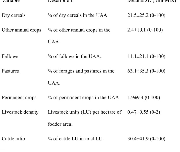
Table S1. Summary statistics of farm characterization variables used to model farming system (n = 7883; UAA = Utilized Agricultural Area).
Variable Description Mean ± SD (Min-Max)
Dry cereals % of dry cereals in the UAA 21.5±25.2 (0-100)
Other annual crops % of other annual crops in the UAA.
2.4±10.1 (0-100)
Fallows % of fallows in the UAA. 11.1±21.1 (0-100)
Pastures % of forages and pastures in the UAA.
63.1±35.3 (0-100)
Permanent crops % of permanent crops in the UAA 1.9±9.4 (0-100)
Livestock density Livestock units (LU) per hectare of fodder area.
0.47±0.55 (0-2)
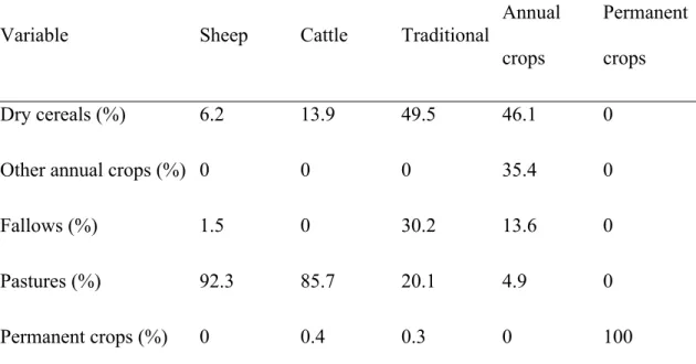
The PAM procedure returned 5 clusters, which were interpreted as farming systems and named on the basis of their main characteristics (Table S2). The Sheep and Cattle systems were identified as livestock specialized systems, mainly differing on the type of livestock and grazing density. The Traditional system was acknowledged as a mixed system, where annual crop production was complemented with low density sheep grazing. This system was identified as a potential representative of the low-intensity cereal-fallow-sheep system that dominated the local landscape for decades, providing the conservation relevant cereal-steppe habitat that lead to the classification of the area as a Special Protection Area under the EU Directive 79/409/CEE (Birds Directive) and to the implementation of an agri-environmental scheme aimed at safeguarding this high nature value farmland (Delgado and Moreira, 2000; Ribeiro et al., 2014). Both the Annual and Permanent crops systems were identified as specialized in crop production, with no livestock, with the former dedicated to arable crops and the later to permanent crops, mostly olive groves.
Table S2. Summary statistics of the five farming systems returned by the PAM cluster analysis. Variable definition in Table S1.
Variable Sheep Cattle Traditional
Annual crops
Permanent crops
Dry cereals (%) 6.2 13.9 49.5 46.1 0
Other annual crops (%) 0 0 0 35.4 0
Fallows (%) 1.5 0 30.2 13.6 0
Pastures (%) 92.3 85.7 20.1 4.9 0
Livestock density (LU/ha)
0.22 0.64 0.19 0 0
Annex B
Table S3. Summary statistics for the biophysical, structural and policy farm characterization variables (n = 7883).
Variables (unit) Code Mean ± SD (Min-Max)
Biophysical
Proportion of good quality soils for agricultural use in the UAA (%)
SOIL 0.15±0.26 (0.00-1.00)
Average slope in the UAA (degrees) SLOPE 3.07±0.89 (1.29-12.60) Average annual rainfall (103 mm) RAIN 0.55±0.06 (0.43-0.68)
Structural
Utilized agricultural area (km2) UAA 1.78±2.13 (0.10-22.07)
Proportion of oak woodlands in the UAA (%)
OAK 0.26±0.30 (0.00-1.00)
Januszewski index (adimensional) JANUS 0.73±0.22 (0.23-1.00) Policy
Location regarding the Special Protection Area of Castro Verde (In=1; Out=0)
SPA 0.45±0.50 (0.00-1.00)
Notes: Soil quality (SOIL), terrain slope (SLOPE), annual rainfall (RAIN) and oak woodlands (OAK) were computed by intersecting the farm parcels layer derived from the LPIS with raster layers of the corresponding spatial distributions ((Fig. S1). Oak woodlands, representing areas occupied by cork oak Quercus suber and holm oak Q. rotundifolia, were included as structural variables because they constrain the range of farm management decisions since cutting these oaks is strongly restricted by Portuguese law. Farm size was computed by the farm’s total Utilized Agricultural Area (UAA), and farm’s spatial fragmentation was quantified with the Januszewski index (JANUS) (Januszewski, 1968; Simion, 2008) calculated from LPIS data, which has been associated with agricultural productivity (Chukwukere Austin et al., 2012). A dummy variable was used to discriminate farms in/outside the SPA of Castro Verde, since SPA regulations prevents the plantation of permanent crops or the expansion of irrigation infrastructures (Santana et al., 2014).
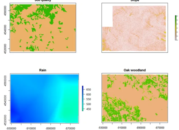
Figure S1. Spatial distribution of the biophysical (soil quality, slope and rain) and structural (Oak woodland) independent variables tested in the models, within the study area.
Soil quality – spatial distribution of soils with good agricultural potential (in green)1; Slope
– terrain slope, values in degrees (source: personal computation based on a digital
elevation model); Rain – average annual precipitation, in mm, computed by interpolating the values from local weather stations2; Oak woodland – spatial distribution of Oak
woodland areas (in green)3.
1 SROA/CNROA, 2012. Carta de Capacidade de Uso do Solo. DGADR - Serviço Reconhecimento e
Ordenamento Agrário.
2 INMG, 1991. Normais climatológicas da Região de "Alentejo e Algarve", correspondentes a 1951-1980.
Instituto Nacional de Meteorologia e Geofísica. O Clima de Portugal, Fascículo XLIX, Volume 4 - 4ª Região. Lisboa.
3 IGP, 2012. Carta de Ocupação do Solo - COS’ 90 [WWW Document]. URL
Fig. S2. Changes in gross income ratio (GIR) between the Traditional farming system and the Cattle, Sheep and the composite Livestock systems during the study period. The value is above 1 when the gross income for the Traditional system is higher than the alternative systems, and below 1 otherwise.
Annex C
Table S4. Agricultural producer prices and direct payments between 1999 and 2011.
1999 2000 2001 2002 2003 2004 2005 2006 2007 2008 2009 2010 2011 Agricultural prices
Common wheat (€/kg) 0.16 0.14 0.16 0.15 0.15 0.17 0.22 0.21 0.18 0.20 0.14 0.15 0.15
Durum wheat (€/kg) 0.18 0.16 0.19 0.18 0.19 0.19 0.23 0.21 0.20 0.27 0.23 0.17 0.20
Sunflower (€/kg) 0.22 0.19 0.28 0.28 0.22 0.22 0.27 0.32 0.32 0.49 0.25 0.28 0.32
Vegetables for industry (€/kg) 0.10 0.10 0.11 0.13 0.13 0.13 0.12 0.13 0.08 0.09 0.09 0.10 0.08
Olives (€/kg) 0.81 0.75 0.67 0.72 0.76 0.89 1.47 1.75 0.40 0.38 0.32 0.30 0.29
Calf 3 to 6 months (€ per live animal) 244.43 243.50 222.94 244.20 243.97 218.09 220.57 266.21 362.14 338.85 362.41 368.37 402.50 Lamb up to 28 kg (€/kg live weight) 2.76 2.82 3.33 3.10 3.13 2.97 2.79 2.83 2.66 2.66 2.81 2.73 2.78 Direct payments
Arable crops (€/ton) 62.00 63.00 63.00 63.00 63.00 63.00 63.00 0 0 0 0 0 0
Set-aside (€/ton) 62.00 63.00 63.00 63.00 63.00 63.00 63.00 0 0 0 0 0 0
Durum wheat supplement (€/ha) 344.50 344.50 344.50 344.50 344.50 344.50 313.00 0 0 0 0 0 0 Suckler cow - base (€ per animal) 200.00 200.00 200.00 200.00 200.00 200.00 200.00 200.00 200.00 200.00 200.00 200.00 200.00 Suckler cow - additional (€ per animal) 30.19 30.19 30.19 30.19 30.19 30.19 30.19 30.19 30.19 30.19 30.19 30.19 30.19 Suckler cow - extensification premium
<=1,4 LU/ha (€ per animal)
100.00 100.00 100.00 100.00 100.00 100.00 100.00 0 0 0 0 0 0 Sheep - base (€ per animal) 21.00 21.00 21.00 21.00 21.00 21.00 21.00 10.50 10.50 10.50 10.50 10.50 10.50 Sheep - additional (€ per animal) 7.00 7.00 7.00 7.00 7.00 7.00 7.00 3.50 3.50 3.50 3.50 3.50 3.50
Olive oil (€/kg) 0.13 0.13 0.13 0.13 0.13 0.13 0.13 0 0 0 0 0 0
Sources: Agricultural prices – Portuguese National Institute of Statistics (INE – Instituto Nacional de Estatística - http://www.ine.pt); Direct payments: Portuguese Cap paying agency (IFAP – Instituto de Financiamento da Agricultura e Pescas - http://www.ifap.min-agricultura.pt).
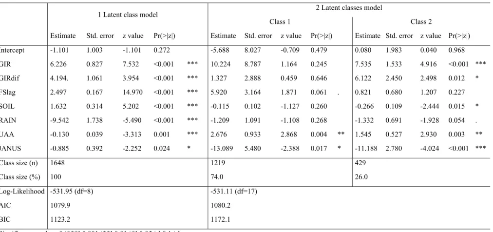
Annex D
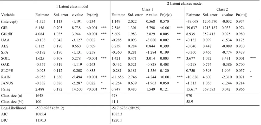
Table S5. Outputs of the latent class model with panel data, including all candidate independent variables (for 1, 2 and 3 latent classes) 2 Latent classes model
1 Latent class model
Class 1 Class 2
Variable Estimate Std. error z value Pr(>|z|) Estimate Std. error z value Pr(>|z|) Estimate Std. error z value Pr(>|z|) (Intercept) -1.325 1.113 -1.191 0.234 1.149 2.022 0.568 0.570 -39.068 1206.570 -0.032 0.974 GIR 6.158 0.705 8.738 <0.001 *** 7.546 1.301 5.798 <0.001 *** 39.637 1213.187 0.033 0.974 GIRdif 4.084 1.035 3.944 <0.001 *** 5.609 1.983 2.829 0.005 ** 8.935 352.413 0.025 0.980 UAA -0.133 0.042 -3.127 0.002 ** -0.285 0.093 -3.080 0.002 ** -0.152 0.099 -1.534 0.125 AES 0.112 0.170 0.660 0.509 0.239 0.284 0.844 0.399 -0.040 0.448 -0.089 0.930 SPA -0.192 0.170 -1.131 0.258 -0.360 0.281 -1.284 0.199 -0.360 0.466 -0.774 0.439 SOIL 1.625 0.308 5.278 <0.001 *** 1.421 0.471 3.014 0.003 ** 3.677 1.072 3.431 0.001 *** OAK -0.357 0.319 -1.119 0.263 -0.432 0.521 -0.828 0.408 -0.298 0.774 -0.386 0.700 SLOPE -0.023 0.112 -0.208 0.835 -0.281 0.181 -1.556 0.120 0.750 0.393 1.906 0.057 . RAIN -8.953 1.630 -5.494 <0.001 *** -11.656 2.746 -4.244 <0.001 *** -10.626 4.600 -2.310 0.021 * JANUS -0.882 0.386 -2.287 0.022 * -1.254 0.639 -1.963 0.050 * -1.313 1.056 -1.244 0.214 FSlag 2.488 0.172 14.503 <0.001 *** 0.747 0.483 1.549 0.121 15.617 369.583 0.042 0.966 Class size (n) 1648 678 970 Class size (%) 100 41.1 58.9 Log-Likelihood -530.6985 (df=12) -517.6736 (df=25) AIC 1085.4 1085.3 BIC 1150.3 1220.5
Table S5. (cont.)
3 Latent classes model
Variable Class 1 Class 2 Class 3
Estimate Std.Error z value Pr(>|z|) Estimate Std.Error z value Pr(>|z|) Estimate Std.Error z value Pr(>|z|) (Intercept) -78.939 38.764 -2.036 0.042 * 138.365 74.060 1.868 0.062 . -3.921 1.866 -2.101 0.036 * GIR 43.783 21.781 2.010 0.044 * 14.548 10.350 1.406 0.160 7.776 1.157 6.723 <0.001 *** GIRdif 7.348 6.946 1.058 0.290 -148.959 79.791 -1.867 0.062 . 6.136 1.635 3.754 <0.001 *** UAA -0.563 0.466 -1.208 0.227 -12.444 6.886 -1.807 0.071 . -0.128 0.074 -1.721 0.085 . AES -3.744 2.242 -1.670 0.095 . -4.853 2.907 -1.669 0.095 . 0.493 0.282 1.751 0.080 . SPA -0.451 1.604 -0.281 0.778 5.963 4.286 1.391 0.164 -0.457 0.275 -1.666 0.096 . SOIL 52.189 29.499 1.769 0.077 . -12.467 6.050 -2.061 0.039 * 2.014 0.559 3.601 <0.001 *** OAK -3.674 2.677 -1.372 0.170 -12.382 7.174 -1.726 0.084 . -0.550 0.504 -1.090 0.276 SLOPE 7.581 3.707 2.045 0.041 * -14.188 7.001 -2.027 0.043 * 0.154 0.192 0.804 0.422 RAIN -57.851 38.800 -1.491 0.136 -223.557 117.598 -1.901 0.057 . -7.078 2.510 -2.820 0.005 ** JANUS -2.440 4.598 -0.531 0.596 -65.361 33.715 -1.939 0.053 . 0.289 0.643 0.449 0.653 FSlag 54.787 29.286 1.871 0.061 . 23.888 11.344 2.106 0.035 * 1.453 0.347 4.190 <0.001 *** Class size (n) 766 212 670 Class size (%) 46,5 12.9 40.7 Log-Likelihood -499.0301 (df=38) AIC 1074.1 BIC 1279.5 Significance codes: 0 ‘***’ 0.001 ‘**’ 0.01 ‘*’ 0.05 ‘.’ 0.1 ‘ ’