Bayesian estimation of genotypic and phenotypic correlations from crop variety trials

Bayesian estimation of genotypic and phenotypic correlations from

crop variety trials

Siraj Osman Omer1*_{, Abdel Wahab H Abdalla}2_{, Mohammed H. Mohammed}3 _{and Murari Singh}4

Received 27 August 2014 Accepted 04 July 2015

Abstract – Genotypic and phenotypic correlations are necessary for constructing indirect selection indices. Bayesian analysis, therefore, was applied to obtain posterior distributions of the correlations, and the estimates were compared with those under a frequentist approach. Three a priori distributions for standard deviation components based on uniform distribution, positive values from t- distribution, and positive values from normal distribution were examined, while a priori distribution for correlation was taken as a uniform distribution. The prior based on uniform was best found using the deviation information criterion. Data from sorghum genotypes evaluated in complete blocks in 2010-2011 in Northern Kordofan, Sudan, resulted in a posterior mean of 0.48 for genotypic correlation between seed yield and seed weight with posterior standard deviation of 0.24. Due to a wider inference base and the fact that it makes use of prior information, we recommend the Bayesian approach in estimation of genotypic correlations.

Key words: Bayesian estimation, genotypic and phenotypic correlations, heritability, R2WinBUGS.

Crop Breeding and Applied Biotechnology 16: 14-21, 2016 Brazilian Society of Plant Breeding. Printed in Brazil

ARTICLE

http://dx.doi.org/10.1590/1984-70332016v16n1a3

1 _{Agricultural Research Corporation (ARC), Experimental Design and Analysis Unit, P.O. Box 126, Wad Medani, Sudan. *E-mail: sirajstat@yahoo.com}

2 _{University of Khartoum, Faculty of Agriculture, Khartoum, Department of Agronomy, Sudan}

3 _{ARC, Cereal Research Center, P.O. Box 126, Wad Medani, Sudan}

4 _{International Center for Agricultural Research in the Dry Areas (ICARDA), P.O. Box 950764, Amman, Jordan}

INTRODUCTION

Genotypic and phenotypic correlations between plant traits are used as measures of their association (Ahmad et al. 2010). Estimates of genotypic and phenotypic correlations between traits are useful in planning and evaluating breeding value (Desalegn et al. 2009). Knowledge of genotypic and phenotypic association among economically valuable traits can help plant breeders in identifying efficient breeding strategies for development of high yielding wheat cultivars (Abbasi et al. 2014). Though estimation of genotypic correlations and phenotypic correlations is straightforward, evaluation of their precision in terms of standard errors and significance testing is quite cumbersome (Singh et al. 1997). Over the course of experimentation, crop improvement programs gather information on genotypic and experimental error variability, which can be used in the Bayesian approach. In the Bayesian framework, one integrates prior information with the likelihood of current data and draws inferences in terms of conditional distribution of parameters of interest, given the data. In this process, an estimate of the parameter is assessed as posterior mean and precision as posterior

standard deviation (Gelman et al. 2004). In contrast, the commonly used frequentist approach does not make use of such information. Singh et al. (2015) have presented a systematic approach for Bayesian analysis of trials conducted in complete or incomplete block designs. The priors discussed in their work have been incorporated in this study. This paper focuses on the Bayesian approach for estimation of genotypic and phenotypic correlations from crop variety trials and compares them with a frequentist approach.

1994). Schisterman et al. (2003) investigated estimation of the correlation coefficient using the Bayesian approach and its applications in epidemiological research and found it useful for evaluating relationships between variables with measurement errors. More details on Bayesian estimation of correlation may be found in Liechty et al. (2004) for models providing a framework for representing and learning about dependence structures. The objective of this study is to estimate genotypic and phenotypic correlations and their standard errors using Bayesian and frequentist approaches when data on traits have been collected from a crop variety trial conducted in a randomized complete block design. The necessary computing codes are also provided using R2WinBUGS and R-packages.

MATERIAL AND METHODS Experimental data

A set of 18 sorghum genotypes were evaluated in a randomized complete block design (RCBD) with four replications. The experiment was carried out in the 2010-2011 season at El Obeid Research Station, Agricultural Research Corporation (ARC), Northern Kordofan, Sudan. Plot-wise data on grain yield in kg ha-1 _{(GY) and 1000 seed}

weight in gm (SW) were recorded.

Estimation of genotypic and phenotypic correlation

Frequentist approach

In this approach, we consider estimation of genotypic correlation from a randomized complete block design (RCBD) data on two traits – X (for example, yield) and Y (for example, seed weight). The ρ_gxy denotes the genotypic correlation between traits X and Y in a population of inbred lines. We consider v inbred lines are randomly selected from the population of interest and are evaluated in an RCBD with r replications in a single environment. The responses X_ij and Y_ij from the plot of the ith _{genotype of the j}th _replicate

are modeled as:

(

x_ij y_ij

)

=

(

μ_x μ_y

)

+

(

β_jx β_jy

)

+

(

g_ix g_iy

)

+

(

εijx

εijy

)

(1)

where for the two traits X and Y, μ_x and μ_y are general means,

βjx and βjy are effects of the j

th _{block, g}

ix and giy are effects of

the ith _{genotype sampled, and} ε

ijx and εijy are random errors,

respectively (Singh and Hinkelmann 1992). The parameter vector

(

μ_x

μy

)

is assumed to be fixed.

However, we make the following assumptions for the other vectors:

1-

(

β_jx

β_jy

)

is bivariate normally distributed with mean vector

(

0

0

)

, a variance-covariance matrix

(

σ 2

βx σβxy

σ_βxy σ 2 βy

)

, and

independent of

(

ββj_j''xy

)

for j ≠ j', j = 1,...,r.

2-

(

g_ix

giy

)

is bivariate normally distributed with mean

vector

(

0

0

)

, a variance-covariance matrix

(

σ 2

βx σβxy

σβxy σ 2βy

)

, and

independent of

(

g_i'x

gi'y

)

for i ≠ i', i = 1,...,v.

3-

(

εεijijxy

)

is bivariate normally distributed with mean

vector

(

0

0

)

, a variance-covariance matrix

(

σ 2

ex σexy

σexy σ

2

ey

)

, and

independent

(

εi'j'x

εi'j'y

)

, where i ≠ j', j ≠ j'.

4- The vectors

(

gix

g_iy

)

,

(

βjx

β_jy

)

, and

(

εεijijxy

)

are pairwise

independent of each other (Singh and Hinkelmann 1992). Given the above background, the genotype correlation between traits X and Y is estimated as:

ρˆ_gxy = σˆgxy

σˆ_gxσˆ_gy (2)

where σˆ_gxy is the estimated genotypic covariance between traits X and Y, σˆ_gx is the estimated genotypic standard deviation for trait X, and σˆ_gy is the estimated genotypic standard deviation for trait Y. Thus, the estimate of ρ_g is obtained in terms of the estimates of the variance and covariance components σ 2

gx, σ

2

gy and σgxy. The variance

components σ 2

gx and σ

2

gy can be estimated by using the

residual (otherwise known as “restricted”) maximum likelihood (REML) method (Patterson and Thompson 1971, Singh et al. 1997). From the covariance σ_gxy obtained, we can construct a new variable Z with the plot-wise values as

Z_ij = X_ij + Y_ij, (3) where,

Z_ij = μ_z + β_jz + g_iz + ε_ijz, where

μz = μx + μy, βjz = βjx + βjy

g_iz = g_ix + g_iy, ε_ijz = ε_ijx + ε_ijy (i = 1,..., v, j = 1,...,r)

The genotypic variability of variable Z, denoted by

σ 2

gz, is expressed as:

σ 2

gz = Var(giz) = Var(gix + giy), or σ

2

gz = σ

2

gx + σ

2

Thus, the covariance component σ_gxy can be written in terms of variance components as

σgxy = (σ

2

gz – σ

2

gx – σ

2

gy)/2 (5)

We now apply the REML method on Z_ij values of Z to obtain an estimate σˆ 2

gz of σˆ

2

gy. Substituting the estimates of

the three variance components in (5), we get an estimate

σˆ_gxy where

σˆ_gxy =(σˆ 2

gz – σˆ

2

gx – σˆ

2

gy)/2

Substituting the estimates of σ 2

gx , σ

2

gy, and σgxy in (2), we

obtain the estimate ρˆ_gxy = σˆ_gxy/(σˆ 2

gx σˆ

2

gy)

1/2

In order to compute phenotypic correlation, we consider the additive model for the phenotypic value - phenotypic value = genotypic value + environmental effect. After ignoring the variation in controlled factors, if any, we can write the phenotypic variances and covariance as follows:

σ 2

px = σ

2

gx + σ

2

ex

σ 2

py = σ

2

gy + σ

2

ey

σpxy = σgxy + σexy

Using equation (3), the covariance σexy can be obtained

from the variance components σ 2

ex, σ

2

ey and σ

2

ez, where z =

x + y using

σ_exy = (σ 2

ez – σ

2

ex – σ

2

ey)/2 (6)

Thus, the phenotypic correlation ρ_pxy and the environmental correlation ρ_exy between the traits X and Y are expressed as:

ρ_pxy = σ_pxy/(σ_pxσ_py) and ρ_exy = σ_exy/(σ_exσ_ey) (7) Standard error of the estimates of phenotypic and environmental correlation can be obtained using Singh et al. (1997) with the delta method. Similar approaches have been described by Miller et al. (1958) using the corresponding variance and covariance components (Fikreselassie et al. 2012). The approach presented here is based on a univariate approach to variables X, Y, and Z=X+Y. An alternative approach is to use a multivariate formulation implemented in several software programs. In our experience, multivariate approaches more often resulted in non-convergence than the univariate approach (e.g., REML method) did. The variance components for X and Y were also used to estimate the broad-sense heritability of the traits on a mean basis, using the expression (h 2

x = σ

2

gx /(σ

2

gx + σ

2

ex /r) for trait X (as for trait Y), where r is the

number of replications; see also Singh el al. (2015). The estimation under the frequentist approach was carried out using Genstat software (Payne 2014).

Bayesian approach

Knowledge of a priori probability distribution of parameters of interest is required for making estimates under the Bayesian paradigm (Kizilkaya et al. 2002). To introduce the subject, consider the Bayesian approach for estimation of a single parameter θ using an observed data vector y = (y₁,...,y_n). One introduces a degree of belief in the parameter θ in terms of its probability distribution function, for example g(θ), called a priori distribution of θ, or simply a prior for θ. The inference about θ is obtained in terms of the probability distribution of θ given the data y and is expressed as p(θ | y)∞g(θ) f (y | θ) and called the a posteriori, or simply a posterior, density function of θ,which is obtainable from the famous Bayes’ Theorem available in standard texts (Ntzoufras 2002, Rowe 2003, Gelman et al. 2004, Robert and Casella 2004). Using this a posteriori density, one can obtain the expected value of θ as an estimate of θ, standard error, and its Bayesian confidence intervals. The posterior distributions for each of ρ_βxy, ρ_gxy, and ρ_exy can be obtained using the following expression for the situation of a general case of s parameters θ₁, θ₂,..., and θ_s. Let us denote the vector θ = (θ₁, θ₂,..., θ_s). Furthermore, let the bivariate data (x, y) be generated on a pair of variables (X, Y) from the probability density function denoted by f(x, y |θ). The a posteriori distribution of θ_k (k = 1, 2…, s) based on an assumed joint a priori distribution g(θ) of θ is given by:

p(θ_k|(x,y))∞

ʃ

...

ʃ

g(θ)f(x,y|θ)dθ₁dθ₂...dθ_k–1dθ_k+1...dθ_s The priors used include uniform, half normal, and gamma distributions for genotypic and phenotypic standard deviation components and uniform distribution for the correlations. Wong et al. (2003) proposed a prior probability model for the precision matrix in the case of multivariate responses. For responses from an RCBD, mixed linear models were used to estimate the variance components (Vargas et al. 2013). In the present context, the parameters of model (1) are μ_x, μ_y, β_jx, β_jy, g_ix, g_iy (the effects), σ_βx, σ_βy, σ_gx, σ_gy,

σex, σey (the standard deviations), and ρβxy, ρgxy and ρexy (the

correlations). Priors are needed for standard deviations and correlations in the above. Following Gelman (2006), we used non-informative priors for scale parameters involved in these correlation parameters as uniform, positive half-t, and positive half-normal families of distributions (Crossa et al. 2010). The following sets of prior distribution were considered.

P₁: the priors for block, genotypic, plot-error standard deviations σ_βx, σ_βy, σ_gx, σ_gy, σ_ex, and σ_ey ~U(0, 100) and the priors for block, genotypic, and environmental correlations

P₂: the priors for block, genotypic, plot-error standard deviations σ_βx, σ_βy, σ_gx, σ_gy, σ_ex, and σ_ey ~positive half normal (0, τ–1_{), and the priors for block, genotypic, and environmental}

correlations ρ_βxy, ρ_gxy and ρ_exy ~U(-0.99, 0.99). Here the precision parameter τ = σ–1 _{is the inverse of the variance.}

P₃: the priors for block, genotypic, plot-error standard deviations

σ_βx, σ_βy, σgx, σgy, σex, and σey ~positive half -t(0, c, υ),

and the priors for block, genotypic and environmental correlations ρ_βxy, ρ_gxy and ρ_exy ~U(-0.99, 0.99). Here c is a non-centrality parameter and υ is the degree of freedom of the t-distribution.

Since there are multiple priors, the best prior distribution was selected using a discrepancy criterion, the deviance information criterion (DIC), commonly considered for prior model selection (Gelman et al. 2004, Griffin and Brown 2012). The inference on the correlations was drawn using the best prior. We used the R2WinBUGS package and R- codes given in the Appendices. The number of iterations was set at 100,000 with three chains, and 5000 simulation values were taken for statistical summaries on the posteriors. Unlike the univariate approach in the frequentist method, here we used a multivariate (bivariate) framework in the Bayesian computations. In the bivariate case, the calculations were carried out by defining the priors at each element of the variance-covariance matrix. Alternatively, particularly with more than two traits, one may use Wishart distribution. RESULTS AND DISCUSSION

Selection of priors

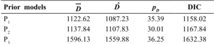
Choices of priors for Bayesian analysis were made from the statistics given in Table 1. Deviance information criteria (DIC) values were 1158.02 for P₁, 1168.11 for P₂, and 1631.9 for P₃. However, the prior set P₁ has the lowest

numerical value of DIC (1158.02); we took P₁ for estimation of the genetic parameters.

Genotypic and phenotypic variance components and heritability

Table 2 shows the frequentist estimates of the genotypic, phenotypic, and environmental variances and their estimated standard errors, as described in Singh and El-Bizri (1992) and the asymptotic 95% confidence intervals. Bayesian estimates are based on the best priors set (P₁) selected using the DIC. The posterior means of genotypic and environmental variance components were higher than the associated estimates in the frequentist version. Estimates of broad-sense heritability on a mean basis followed a similar trend, with Bayesian vs frequentist approach estimates as 0.94 vs. 0.95 for GY and 0.67 vs. 0.70 for SW.

Genotypic, phenotypic, and environmental correlations

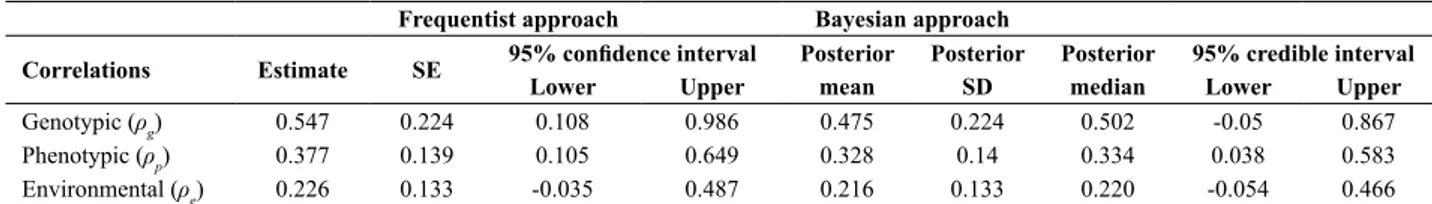
For the frequentist approach, Table 3 presents estimates, estimated standard errors, and asymptotic confidence intervals of the genotypic, phenotypic, and environmental correlations between GY and SW, whereas for Bayesian and frequentist approaches, it presents their posterior means, standard deviations, and medians, along with credible and confidence intervals. Genotypic, phenotypic, and environmental correlations between GY and SW under the frequentist vs. Bayesian approach were 0.547 vs. 0.475, 0.377 vs. 0.328, and 0.226 vs. 0.216, respectively. A comparison between means and median showed that the Bayesian posterior distributions of these correlations are slightly skewed. The precision levels of various correlations were reasonably close for the two approaches.

Sorghum genotypes considered in the trial showed significant genetic variability for grain yield (GY) and 1000 seed weight (SW). The study makes use of prior information in terms of distributions of various variance components that may be made available from an ongoing series of crop variety trials. How the information can be utilized has been shown by the Bayesian approach, which integrates the prior information with the likelihood of the current datasets, so as to draw inferences on genotypic, phenotypic, and environmental correlations. Variable degrees of differences between the Bayesian and frequentist approaches have been found in the precision levels of the estimates of variance-component-based parameters in other studies (Singh et al. 2015). In the case of the Bayesian approach, the precision associated with a parameter depends on the priors used. The merit of the Bayesian approach depends on the premise of its allowing for a realistic coverage of the distribution of

Table 1. Discrepancy statistics for selection of the priors for the 2010-11 dataset

Prior models _D Dˆ p_D DIC

P₁ 1122.62 1087.23 35.39 1158.02

P₂ 1137.84 1107.83 30.01 1167.84

P₃ 1596.13 1559.88 36.25 1632.38

Where D=posterior mean of (- 2 × log-likelihood). Dˆ= - 2 × log-likelihood at pos-terior means of parameters. pD= effective number of parameters, DIC= Deviance information criterion. Priors set are:

P₁: σ_βx, σ_βy, σ_gx, σ_gy, σ_ex, and σ_ey ~U(0, 100) ; ρ_βxy, ρ_gxy and ρ_exy~U(-0.99, 0.99). P2: σβx, σβy, σgx, σgy, σex, and σey ~positive half normal (0, τ

–1_); ρ

βxy, ρgxy and ρexy ~U(-0.99, 0.99).

various parameters used as priors. The Bayesian approach may not necessarily result in a lower posterior standard deviation of a parameter in comparison to the standard error of estimate of the parameter in the frequentist approach. Such investigations need to be carried out on other datasets to make an assessment of trends in the precision obtained by these two approaches. The most commonly used priors for variance components in terms of the standard deviation components have been used (Gelman 2006), but classes of other relevant priors (Crossa et al. 2010) may also be included to examine support from data using the deviance information criterion. The simulation in the Bayesian approach using the R2WinBUGS software (Spiegelhalter et al. 2002) enables evaluation of the posterior distribution of the derived correlations in terms of variance and covariance components, unlike the frequentist methods where the simplification of the distribution is commonly made as asymptotic approximation (Singh and El- Bizri 1992). The R2WinBUGS software facilitated summaries in terms of posterior mean and median to make inferences regarding the symmetry of the distributions and the percentiles in reporting the credible intervals. Bayesian computation can also use the information from the experimental units that have data on additional units for only a single trait (broken samples) to estimate the genotypic and phenotypic correlations and the variance components for those traits. Furthermore, study in Bayesian estimation should be extended to multivariate

cases (with more than two traits) in future investigations in plant breeding. Accordingly, heterogeneity in environmental variances and in genotype variances should also be the aspect of a future study by considering suitable models for heterogeneity of variances.

In summary, this study presents the Bayesian approach for estimation of genotypic and phenotypic correlations between traits from crop variety trials using the priors on standard deviation components and correlations obtainable from a series of previously conducted trials. The R2WinBUGS software was used for Bayesian estimates of genotypic and phenotypic correlations using experimental design data. Uniform distribution based on the priors set was found to be best, which led to precision similar to the frequentist approach. Due to its sound inference base, the Bayesian approach with WinBUGS and R codes is recommended for use in estimation of genotypic correlation in plant breeding trials.

ACKNOWLEDGMENTS

The authors are thankful to the reviewer for his/her suggestions which led to substantial improvement of the earlier version of the manuscript. The first author is grateful to ICARDA and the Arab Fund for Economic and Social Development (AFESD) for granting a fellowship for carrying out the research study.

Table 2. Estimates of variance components and broad-sense heritability on a mean basis for grain yield and 1000 seed weight under the frequentist

and Bayesian approach for the 2010-11 dataset

Frequentist approach Bayesian approach

Parameters Estimate SE 95% confidence interval Posterior Posterior Posterior 95% credible interval Lower Upper mean SD median Lower Upper

Grain

yield(GY)

σ 2

ex 1071 212 655 1487 1155 238.8 1125 778.9 1712

σ 2

gx 4642 1685 1339 7945 5315 1735 5050 2625 9196

h 2

x 0.95 0.022 0.91 0.99 0.94 0.023 0.95 0.89 0.97

1000 seed (SW)

σ 2

ey 18.06 3.58 11.04 25.08 20.13 4.34 19.53 13.28 30.48

σ 2

gy 10.46 5.21 0.25 20.67 12.26 7.08 10.93 2.548 29.09

h 2

y 0.7 0.119 0.47 0.93 0.67 0.15 0.69 0.3 0.87

SE: Standard error. SD: standard deviation. The SE and 95% confidence intervals for the frequentist approach estimates are based on asymptotic normal approximation.

Table 3. Estimates of genotypic (ρ_g),phenotypic (ρ_p), and environmental (ρ_e) correlations between grains yield (GY) and 1000 seed weight (SW) under

frequentist and Bayesian approaches for the 2010-11 dataset

Frequentist approach Bayesian approach

Correlations Estimate SE 95% confidence interval Posterior Posterior Posterior 95% credible interval Lower Upper mean SD median Lower Upper

Genotypic (ρ_g) 0.547 0.224 0.108 0.986 0.475 0.224 0.502 -0.05 0.867

Phenotypic (ρ_p) 0.377 0.139 0.105 0.649 0.328 0.14 0.334 0.038 0.583

Environmental (ρe) 0.226 0.133 -0.035 0.487 0.216 0.133 0.220 -0.054 0.466

REFERENCES

Abbasi S, Baghizadeh A, Mohammadi-Nejad G and Nakhoda B (2014) Genetic analysis of grain yield and its components in bread wheat

(Triticum aestivum L.). Annual Research & Review in Biology

24: 3636-3644.

Ahmad B, Khalli IH, Igbal M and Ur-Rahman H (2010) Genotypic and phenotypic correlation many yield components in bread wheat under normal and late planting. Sarhad Journal of Agriculture 26: 259-265.

Crossa J, de los Campos G, Pérez P, Gianola D, Burgueño J, Araus JL, Makumbi D, Singh RP, Dreisigacker S, Yan J, Arief V, Banziger M

and Braun HJ (2010) Prediction of genetic values of quantitative traits

in plant breeding using pedigree and molecular markers. Genetics 186: 713-724.

Desalegn Z, Ratanadilok N and Kaveeta R (2009) Correlation and

heritability for yield and fiber quality parameters of Ethiopian

cotton (Gossypium hirsutum L.) estimated from 15 (diallel) crosses.

Kasetsart Journal Natural Science 43: 1-11.

Fikreselassie M, Zeleke H and Alemayehu N (2012) Correlation and path analysis in Ethiopian fenugreek (Trigonella foenum-graecum L.) landraces. Crown Research in Education 3: 132-142.

Gelman A, Chew GL and Shnaidman M (2004) Bayesian analysis of serial dilution assays. Biometrics 60: 407-417.

Gelman A (2006) Prior distributions for variance parameters in hierarchical models. Bayesian Analysis 3: 515-533.

Griffin JE and Brown PJ (2012) Structuring shrinkage: some correlated

priors for regression. Biometrika 99: 481-487.

Hussain K, Khan IA, Sagat HA and Amjad M (2012) Genotypic and

phenotypic correlation analysis of yield and fiber quality determining

traits in upland cotton (Gossypim hirsutum). International Journal of Agricultural and Biology 12: 348-352.

Kizilkaya K, Banks BD, Carnier P, Albera A, Bittante G and Tempelman RJ (2002) Bayesian inference strategies for the prediction of genetic merit using threshold models with an application to calving ease scores in Italian Piemontese cattle. Journal of Animal and Breeding Genetics 119: 209-220.

Liechty JC, Liechty MW and Muller P (2004) Bayesian correlation estimation. Biometrika 91: 1-14.

Littell RC, Henry PR and Ammerman CB (1998) Statistical analysis of repeated measures data using SAS procedures. Journal of Animal Science 76: 1216-1231.

Miller PA, Williams JC, Robinson HF and Comstock RE (1958) Estimates of genotypic and environmental variances and covariances in upland cotton and their implications in selection. Agronomy Journal 50:

126-131.

Ntzoufras I (2002) Gibbs variable selection using BUGS. Journal of Statistical Software 7: 1-19.

Patterson HD and Thompson R (1971) Recovery of inter-block information

when block sizes are unequal. Biometrika 58: 545-554.

Payne RW (2014) The guide to GenStat® command language (Release 17). Part 2: Statistics. VSN International, Hemel Hempstead, 1032p. R Development Core Team (2009) R: A language and environment

for statistical computing. R Foundation for Statistical Computing, Vienna, 409p.

Robert C and Casella G (2004) Monte Carlo statistical methods. 2nd _edn, Springer-Verlag, New York, 645p.

Rowe DB (2003) Multivariate Bayesian statistics: Models for source separation and signal unmixing. Chapman & Hall/CRC, New York, 352p.

SAS Institute (2011) SAS/STAT® 9.2 User’s guide. 2nd _{edn,SAS Institute,} Cary, 7869p.

Schisterman EF, Moysich KB, England LJ and Rao M (2003) Estimation

of the correlation coefficient using the Bayesian approach and its

applications for epidemiologic research. BMC Medical Research Methodology3: 1-5.

Singh M, Al-Yassin A and Omer S (2015) Bayesian estimation of genotypes means, precision and genetic gain due to selection from routinely used barley trials. Crop Science55: 501-513.

Singh M and El-Bizri KS (1992) Phenotypic correlation: its estimation

and test of significance. Biometrical Journal 43: 165-171. Singh M, Ceccarelli S and Grando S (1997) Precision of the genotypic

correlation estimated from variety trials conducted in incomplete block designs. Theoretical and Applied Genetics 95: 1044-1048. Singh M and Hinkelmann K (1992) Distribution of genotypic correlation

coefficient and its transforms for non-normal populations. Sankhya Series B 54: 42-66.

Spiegelhalter DJ, Best NG, Garlin BA and Van der Linde A (2002)

Bayesian measures of model complexity and fit (with discussion).

Journal of the Royal Statistical Society 64: 583-639.

Tierney L (1994) Markov chains for exploring posterior distributions (with discussion). Annual Statistics 22: 1701-1786.

Vargas M, Combs E, Alvarado G, Atlin G, Mathews K and Crossa J (2013) META: A suite of SAS programs to analyze multi-environment breeding trials. Agronomy Journal 105: 11-19.

Wong F, Carter CK and Kohn R (2003) Efficient estimation of covariance

Appendix A. R-codes for Bayesian analysis of genotypic, phenotypic, and environmental correlations #load packs

library(lattice( library(coda( library(R2WinBUGS(

#Data file has columns for replicates (Rep), genotypes (Geno), grain yield (GY) and thousand seed weight (SW)

data<- read.table(“DataFile.txt”, header=TRUE( rp<- data$Rep # rp for replication vector gn<- data$Geno # gn for genotype vector z <- array(0, dim=c(72,2))

z[,1]<- data$GY z[,2]<- data$SW NB<- 4 NG<- 18 N<- NB*NG print(cbind(z,rp,gn)) print(cbind(NB, NG, N ))

mn <- matrix(0,1, 2) mn[1:2]<- colMeans(z[,1:2])

data<- list(“z”,”rp”,”gn”,”N”, “NB”, “NG») data

inits1<- list(m=c(2,1), b=structure(.Data=c(rep(.01,NB), rep(0.01,NB)), .Dim=c(NB,2)) , g=structure(.Data=c(rep(.021, NG), rep(0.01,NG)),. Dim=c(NG,2)), sig1.e=1, sig2.e=.5, rhoe=.0, sig1.b=1, sig2.b=.5, rhob=.0, sig1.g=1, sig2.g=.25, rhog=.41 )

inits2<- list(m=c(2,1), b=structure(.Data=c(rep(.01,NB), rep(0.01,NB)), .Dim=c(NB,2)),g=structure(.Data=c(rep(.021, NG), rep(0.01,NG)),. Dim=c(NG,2)), sig1.e=1,sig2.e=.5,rhoe=.0, sig1.b=.51, sig2.b=.5, rhob=.0, sig1.g=1, sig2.g=.25, rhog=.01)

inits3<- list(m=c(2,1), b=structure(.Data=c(rep(.01,NB), rep(0.01,NB)), .Dim=c(NB,2)),g=structure(.Data=c(rep(.021, NG), rep(0.01,NG)),. Dim=c(NG,2)), sig1.e=1,sig2.e=.5, rhoe=.0, sig1.b=1.2, sig2.b=.5, rhob=.0, sig1.g=1, sig2.g=.25, rhog=-.11 )

inits <- list(inits1, inits2, inits3) inits

parameters <- c(“m”, “Sig2.b”, “Sig2.g”, “Sig2.e”, “sig2p”, “h2”, “rhog”,”rhoe”, “rhop”) parameters

Appendix B. WinBUGS codes for Bayesian analysis of genotypic correlation

# Text file GCorr.bug

model{

for (i in 1 :N){ z[i,1:2] ~ dmnorm(mu[i,1:2], Tau.e[1:2,1:2]) for(j in 1:2){ mu[i,j]<- m[j] + b[rp[i],j] + g[gn[i],j] } }

# Bivariate errors: variance-covariance matrix (Other option is via Wishart distribution) Sig2.e[1,1]<- sig1.e*sig1.e

Sig2.e[2,2]<- sig2.e*sig2.e Sig2.e[1,2]<- rhoe*sig1.e*sig2.e Sig2.e[2,1]<- rhoe*sig1.e*sig2.e Tau.e[1:2, 1:2]<- inverse(Sig2.e[1:2,1:2]) # priors of error sigmas and rhos sig1.e ~ dunif(0, 100) sig2.e ~ dunif(0, 100) rhoe ~ dunif(-0.99, 0.99)

# two univariate overall means, as fixed effects, m[1:2]

for(i in 1:2) { m[i] ~ dnorm(0.0, 1.0E-06) }

# Bivariate block effects: variance-covariance matrix (Other option is via Wishart distribution) m0[1]<- 0 ; m0[2]<- 0

for (i in 1: NB){b[i,1:2] ~ dmnorm(m0[1:2], Tau.b[1:2,1:2]) } Sig2.b[1,1]<- sig1.b*sig1.b

Sig2.b[1,2]<- rhob*sig1.b*sig2.b Sig2.b[2,1]<- rhob*sig1.b*sig2.b Sig2.b[2,2]<- sig2.b*sig2.b

Tau.b[1:2, 1:2]<- inverse(Sig2.b[1:2,1:2]) # priors of error sigmas and rhos sig1.b ~ dunif(0, 100) sig2.b ~ dunif(0, 100) rhob ~ dunif(-0.99, 0.99)

# Bivariate genotype effects: variance-covariance matrix (Other option is via Wishart distribution) for (i in 1: NG){g[i,1:2] ~ dmnorm(m0[1:2], Tau.g[1:2,1:2]) }

Sig2.g[1,1]<- sig1.g*sig1.g Sig2.g[1,2]<- rhog*sig1.g*sig2.g Sig2.g[2,1]<- rhog*sig1.g*sig2.g Sig2.g[2,2]<- sig2.g*sig2.g

Tau.g[1:2, 1:2]<- inverse(Sig2.g[1:2,1:2]) # priors of error sigmas and rhos sig1.g ~ dunif(0, 100) sig2.g ~ dunif(0, 100) rhog ~ dunif(-0.99, 0.99)

# Prediction of parameters of interest-- phenotypic variances and correlation, broad-sense heritability on mean-basis sig2p[1]<- sig1.g*sig1.g + sig1.e*sig1.e

sig2p[2]<- sig2.g*sig2.g + sig2.e*sig2.e

rhop<- (rhog*sig1.g*sig2.g + rhoe*sig1.e*sig2.e)/sqrt(sig2p[1]*sig2p[2])

h2[1]<- sig1.g*sig1.g / (sig1.g*sig1.g + sig1.e*sig1.e/NB) h2[2]<- sig2.g*sig2.g / (sig2.g*sig2.g + sig2.e*sig2.e/NB) }