An ef®cient BE iterative-solver-based substructuring algorithm for 3D time-harmonic problems in elastodynamics

An ef®cient BE iterative-solver-based substructuring algorithm for 3D

time-harmonic problems in elastodynamics

F.C. ArauÂjo

*, C.J. Martins

, W.J. Mansur

a_{Department of Civil Engineering, Escola de Minas, UFOP, CEP 35400-000, Ouro Preto-MG, Brazil} b_{PEC/COPPE/UFRJ, CXP 68506, CEP 21945-970, Rio de Janeiro, Brazil}

Received 18 May 2000; accepted 13 December 2000

Abstract

This work is concerned with the development of an ef®cient and general algorithm to solve frequency-domain problems modelled by the boundary element method based on a sub-region technique. A speci®c feature of the algorithm discussed here is that the global sparse matrix of the coupled system is implicitly considered, i.e. problem quantities are not condensed into interface variables. The proposed algorithm requires that only the block matrices with non-zero complex-valued coef®cients be stored and manipulated during the analysis process. In addition, the ef®ciency of the technique presented is improved by using iterative solvers. The good performance of pre-conditioned iterative solvers for systems of equations having real-valued coef®cients, well demonstrated in the literature, is con®rmed for the present case where the system matrix coef®cients are complex. The ef®ciency of the algorithm described here is veri®ed by analysing a soil±machine foundation interaction problem. CPU time and accuracy are the parameters used for estimating the computational ef®ciency.q_{2001 Elsevier Science} Ltd. All rights reserved.

Keywords: Boundary element method; 3D Elastodynamics; Frequency-dependent problems; Iterative solvers; Complex non-Hermitian matrices; Substructur-ing technique

1. Introduction

The pioneer work by Cruse [1] was the ®rst to establish the mathematical basis for numerical modelling of elastic wave propagation problems by the boundary element method. Cruse [1] used integral equations in the Laplace transformed domain and a numerical algorithm of inversion due to Papoulis [2] to obtain time-domain responses. It is important to mention that presently Durbin's [3] inversion algorithm is employed rather than Papoulis' [2].

Cruse's [1] work inspired later on the development of BEM models based on the Fourier transform. The derivation of a BEM approach in Fourier domain was straightforward (see Ref. [4]) as such a formulation could be easily derived from Cruse's [1] work by replacing the complex Laplace parametersby iv. FFT algorithms of inversion were used in this case to ®nd time-domain solutions.

BEM procedures based either on Laplace or Fourier transforms (see Ref. [5]) have remained as important alternatives to time-domain BEM formulations (see Refs. [6,7,5]). They are useful alternatives to standard

domain BEM approaches and essential either when time-domain fundamental solutions have not been obtained but the corresponding frequency (or Laplace) domain ones are known, or when physical properties are frequency-dependent. A complete review of the main contributions up to 1996 to the topic boundary element methods in dynamic analysis can be found in Beskos [8,9].

The present paper is concerned with the development of a general and ef®cient BEM sub-region approach to analyse soil±machine foundation interaction. Only harmonic loads are considered here, however, transient excitations can also be dealt with as a trivial extension of the harmonic case [1,4]. Frequency-domain engineering analyses of in®nite domain problems can be conveniently carried out by the boundary element method or by BEM/FEM coupling algo-rithms. Frequency-domain approaches deal with complex-valued variables that are commonly used to describe amplitude and phase angle of both loading and response. Real engineering analyses may require modelling non-homogeneous in®nite media, e.g. soil±structure interaction problems. When the soil is composed of horizontal layers, simple procedures can be employed leading to very economic and accurate numerical models, e.g. models based on superposition of planes waves [10]. However,

0955-7997/01/$ - see front matterq_{2001 Elsevier Science Ltd. All rights reserved.} PII: S 0 9 5 5 - 7 9 9 7 ( 0 1 ) 0 0 0 6 1 - 3

www.elsevier.com/locate/enganabound

when layers are not horizontal, more general procedures must be used [11], BEM being one of the most suitable. In this case, the BE region must be discretized using the sub-region technique.

As it is well known, substructuring strategies extend considerably the range of applications of boundary-integral-based methods. General aspects of sub-regions techniques can be found in known textbooks on boundary element methods [12,13]. More speci®c aspects concerning sub-structuring techniques, which are mainly related to the ef®cient solution of the blocked, sparse, and unsymmetrically coupled ®nal systems, are addressed to in a series of papers published in the last 20 years [14±19]. These works adopt either non-condensed or condensed strategies and are based on the use of direct solvers. In this paper, a non-condensed iterative-solver-based strategy is presented.

Ef®cient procedures must be used in order to analyse complex problems in small computers. The algorithm must use the minimum storage area and yet be fast. These two topics are addressed to in this paper. Storage area is reduced to a minimum by not storing null coef®cients and iterative solvers are used to reduce CPU time. The good performance of iterative solvers for real-valued coef®cient systems of Eqs. (20)±(23) is also con®rmed for the present case, where the system matrix coef®cients are complex.

2. Frequency-dependent boundary integral equations

When the analysis is frequency-dependent the originally time-dependent problem can be converted to an only-boundary value problem governed by

cik…j†Ui…j;v†1 Z

G

Pikp…x;j;v†Ui…x;v†dG…x†

ˆZ GU

p

ik…x;j;v†Pi…x;v†dG…x† 1

Z

V

Uikp…x;j;v†Bi…x;v†dV…x†; …1†

wherecikis the integral-equation jump term, equal to jump

terms for elastostatics, and Upik…x;j;v† andPikp…x;j;v† are

the frequency-dependent fundamental solutions given by

Uikp…x;j;v† ˆ

1 4prr

(

…3r;_ir;_k2dik†

£ "

1

r2_v2 e iv…r=c2†

2eiv…r=c1† !

2 i

rv

1

c2

eiv…r=c2† 2 1

c1

eiv…r=c1† !#

1r;ir;k

1

c2₁ e

iv…r=c1†₂ 1

c2₂ e

iv…r=c2† !

1dik

1

c2₂ e

iv…r=c2† !)

…2†

and

Ppik…x;j;v† ˆ

nm

4pr2

£ (

26c22…5r;ir;kr;m2dikr;m2dkmr;j2dmir;k†

£ "

1

r2v2 e

iv…r=c2†_2eiv…r=c1† !

2 i

rv

1

c2

eiv…r=c2†₂ 1

c1

eiv…r=c1† !#

12

£…6r;_ir;_kr;_m2dikr;m2dkmr;i2dmir;k†

£ eiv…r=c2† 2 c

2 2

c2₁ e

iv…r=c1† !

22iv

c₂r;ir;kr;m£ e

iv…r=c2† 2 c

3 2

c3 1

eiv…r=c1† !

2r;_kdim 122

c2₂ c2₁

!

12iv r

c1

!

eiv…r=c1†

2…r;_mdik1r;idkm† 12iv

r c₂

!

eiv…r=c2†

)

:

…3†

When known complex boundary conditions

U…x;v† ˆ_{U…x;v† ifx[G}

1; …4†

and

P…x;v† ˆ_{P…x;v† ifx[G}

2; …5†

are considered, the boundary integral Eq. (1) gives the complete boundary solution of the frequency-dependent problem (in terms of its complex amplitudes).

Adopting usual discretization procedures, the boundary integral Eq. (1) is converted to the following frequency-dependent system of algebraic equations:

H…v†U…v† ˆG…v†P…v†; …6†

after introducing the boundary conditions shown in Eqs. (4) and (5), Eq. (6) can be written as

A…v†x…v† ˆb…v†; …7†

whose complex solution vectorx…v†contains the unknown boundary values.

indirectly by means of the rigid body displacement criterion. In order to apply this criterion to frequency-dependent problems, the following relationship must be considered [25]:

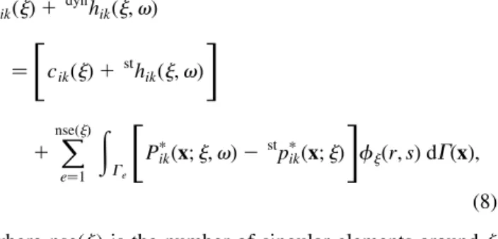
cik…j†1 dynhik…j;v†

ˆ

"

cik…j†1 sthik…j;v† #

1 X

nse…j†

eˆ1

Z

Ge "

Ppik…x;j;v†2 stppik…x;j† #

fj…r;s†dG…x†;

…8†

where nse(j) is the number of singular elements aroundj

and

fj…r;s†

is the shape function related to the singular point. Thus the diagonal block matrices coef®cients for frequency-dependent problems are then determined from the sum of the DBMC for a similar elastostatic analysis Ð obtained by means of the rigid body displacement criterion Ð plus contributions of non-singular integrals as indicated by RHS of Eq. (8). Superscripts st and dyn on expression (8) stand for statics and dynamics, respectively.

Another important point to be observed is that in the case of semi-in®nite domain problems a special mesh of enclos-ing elements must be considered in order to apply the rigid body displacement criterion [11]. Discrete Fourier trans-form (DFT) and inverse discrete Fourier transtrans-form (IDFT) algorithms can be employed to solve time-dependent problems in in®nite or semi-in®nite domains, however in this paper, only steady-state problems were considered.

3. The BE/BE coupling algorithm

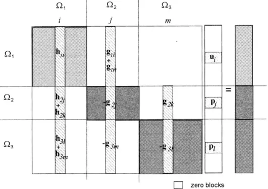
In order to illustrate how the algorithm described in this

section works, the system matrix corresponding to a domain divided into the three sub-domains shown in Fig. 1, is depicted in Fig. 2. In fact the procedure followed in the present paper is quite general, i.e. one can have as many substructures as one wishes. Points 1 and 2 below, and the comments presented subsequently describe the most impor-tant features concerning the assemblage of the ®nal system matrixA…v†shown in Eq. (7).

1. Compatibility and equilibrium conditions, which for instance at the interface between subregions i and j are given by

ui…x† ˆuj…x†; ifx[Gij …9†

and

pi…x† ˆ2pj…x†; if x[Gij …10†

must be introduced.

2. A search in order to identify the coupled nodes must be carried out. It should be noticed that in the proposed algo-rithm, a node cannot be coupled with more than one other. As described in Fig. 1, nodeiis coupled with nodej, nodek

with node l, and node m with node n. By introducing, however, existing traction continuity conditions at nodesi,

j,k,l,m, andnthe corresponding columns inG…v†matrix can be superimposed, such that e.g. for the coupled domain shown in Fig. 1 (with three subdomains), at common inter-face nodes, indeed just two traction vectors…piandpk†must be calculated. One has therefore, at the common node three equations, from which the unknown vectors

uiˆujˆukˆulˆumˆun; …11a†

piˆ2pjˆ2pmˆpn; …11b†

and

pkˆ2pl; …11c†

can be calculated. In general it is valid: at a node common to

n sub-regions, there are n equations for determining one F.C. ArauÂjo et al. / Engineering Analysis with Boundary Elements 25 (2001) 795±803

displacement vector and (n21) traction vectors. Thus, it is necessary that at least one sub-region be smooth at the common node, what represents no restriction to the coupling algorithm proposed here, as it is always possible to create an extra subregion with a smooth boundary, whenever neces-sary.

A simple and important detail of the present coupling formulation, mainly in what concerns the performance of the iterative schemes, is that, in order to obtain better convergence rates, one must use a scaling factor. The one used here is de®ned by

f ˆ 1

ns

Xns

iˆ1

fi; fiˆ

2Gi

…122ni†

; …12†

where ns is the number of sub-regions and Gi andni are,

respectively, the Young's modulus and Poisson's ratio of theith sub-region._{f;given by Eq. (12), is used to scale the}

coef®cients of theG-matrix, such that all coef®cients of the resulting coupled system become of same order of magni-tude. It should be also observed that as a matter of fact, the coupled domain depicted in Fig. 1 is not restricted to 2D problems, as it might seem to be; it refers to 3D problems as well, which in fact constitute exactly the class of problems being treated in this paper.

4. Iterative solvers for complex-valued coupled systems

Iterative procedures for obtaining the solution of systems of algebraic equations have played a very important role in the analysis of engineering problems. They can be of

funda-mental importance to minimise the high analyses costs normally involved in solving algebraic systems, which are sometimes sparse and have a number of equations varying from a few hundreds to a few millions. Important character-istics of iterative procedures that are closely related to their effectiveness are that, besides preserving matrix sparsity, they reduce substantially the CPU time in case of large systems of equations. The gain introduced by iterative solvers is more substantial for algorithms which employ parallel processing strategies. In this case, direct solvers are really inef®cient. A comprehensive study on general aspects of iterative procedures, containing the main devel-opments on this subject in the last decades (until the begin-ning of the 1990s) is presented by Hageman and Young [26] and Hackbusch [27].

Among the iterative schemes, those based on conjugate gradient acceleration procedures [26] have specially attracted the attention of the numerical analysis community. Conjugate gradient methods have a number of favourable properties, three of them being worthwhile mentioning here: (1) though an iterative scheme, convergence is achieved in a ®nite number of iterations if no round-off errors are present, (2) they converge at least as fast as the corresponding Chebyshev procedure, (3) no parameter estimate is neces-sary for obtaining optimal convergence rates.

Concerning BE analyses, nonsymmetric systems of algebraic equations are produced and therefore the develop-ment of iterative solution strategies naturally becomes a much more dif®cult task than in symmetric cases, as reported in works published during the 1980s [28±31]. In the late 1980s, and at the beginning of the 1990s, successful F.C. ArauÂjo et al. / Engineering Analysis with Boundary Elements 25 (2001) 795±803

applications of iterative solvers in BE analyses were reported in works by ArauÂjo and Mansur [20±22,32], in which many different iterative techniques were considered. These works showed that the iterative strategies based on the biconjugate gradient (BiCG) and Lanczos procedures [20,22], with preconditioning, performed especially well in all analyses carried out. Another important point concern-ing these algorithms is that only information related to two previous iterations at most (Lanczos algorithm) is neces-sary. Other methods which require the entire history of iterations or, at least, a great deal of informations concern-ing previous iterations, have also been used successfully, e.g. idealised generalised conjugate gradient acceleration procedures and their corresponding truncated versions [32±35].

In the present paper, the biconjugate gradient algorithm, derived previously for real nonsymmetric and nonsingular matrices [20,22,32], is extended for complex-valued, non-Hermitian systems of algebraic equations.

4.1. Lanczos tridiagonalization algorithm

The starting point for deriving the biconjugated gradient algorithm employed here is the Lanczos tridiagonalization algorithm [32,36]. Starting from two known vectorsc1 and

p_c1_{; both in the N-dimensional complex space C}N

; it is possible by means of the Lanczos tridiagonalization algo-rithm (in the same fashion as for real matrices [32,36]) to derive fromAandAT inCN;Ntwo vector sequences {ck11} and {p_ck11_{};respectively given by}

dk11ck11ˆAck2akck2bkck21 …13†

and

p_d

k11pck11ˆATpck2akpck2pbkpck21: …14†

These are mutually orthogonal to each other, i.e.ck11' p_c1

;pc2;¼;pck and pck11

'c1;c2;¼;ck: It should be observed that these orthogonality conditions, can be used to demonstrate that these two vector sequences are linearly independent for k#N; N being the dimension of the

complex space in question. Thus the following property must be veri®ed:

cN11 ˆpcN11 ˆ0[CN: …15†

The property of Lanczos vectors expressed by Eq. (15) is very important as it is exactly that one used for establishing the ®nite termination of the associated iterative schemes [26,32]. Moreover, if an usual inner product, i.e. not a Hermitian inner product, between complex-valued vectors is used, expressions for determining parametersak;bkand p_b

k in Eqs. (13) and (14) similar to those for real matrices

are obtained; these parameters are computed by [32,36]

akˆ

p_ck;T_Ack

p_ck;T_ck ; …16†

bkˆ

p_ck21;T_Ack

p_ck21;T_ck21; …17†

p_b

kˆ

ck21;TATpck

ck21;Tp_ck21 : …18†

4.2. Bi-conjugate iterative method

Following the same ideas presented by ArauÂjo and Mansur [20±22] and ArauÂjo [32], it is then possible, starting from Eqs. (13), (14), (16)±(18), to derive the Lanczos accel-eration procedure and the bi-conjugate gradient method, the later being given by the following recursive expressions [26,32]:

xn11ˆxn1lnp n

; …19†

pnˆ r

0

; ifnˆ0 rn1anpn21; ifn$1 (

: …20†

rnˆrn212ln21Ap

n21_{; …21†}

By considering now the auxiliary formulas related toAT; F.C. ArauÂjo et al. / Engineering Analysis with Boundary Elements 25 (2001) 795±803

x

y z

Enclosing Elements

6.08 m 6.08 m

1.52 m

1.52 m

1.52 m 6.08 m 6.08 m

1.52 m

5.00 m

which are,

p_rn

ˆprn212ln21ATppn21; …22†

p_pn_ˆ

p_r0 _ˆr0_;

ifnˆ0

p_rn 1anpp

n21_{; ifn}

$1 ;

(

…23†

and using the orthogonality condition of the Lanczos vectors (residue vectors) expressed by

ri;Tprjˆ0; ifi±j; …24†

one can demostrate [32] the A-orthogonality condition of the search direction vectorspi;

p_pi;T_Apj

ˆ0; ifi±j: …25†

Moreover, with aid of these orthogonality conditions (relationships (24) and (25)), the following expressions for parametersln21 andan are obtained [32]:

ln21ˆ

p_rn21;T_rn21

p_pn21;T_Apn21 …26†

anˆ

p_rn;T_rn

p_rn21;T_rn21: …27†

Solvers based on iterative formulas (19)±(23) and (26), (27) are known as bi-conjugate gradient methods and were originally introduced by Fletcher [37].

As one can see with aid of property (24), it is naturally expected that the complex-valued residue vector rn11 becomes identically null for nˆN (c.f. Eq. (15)). This is indeed nothing else than the complete demonstration of convergence of the procedure. For ill-conditioned systems of algebraic equations, despite the ®nite termination property of the iterative scheme, as a consequence of trun-cation errors introduced during the computer data proces-sing, it may happen that convergence is not achieved for

n#N:It does happen that the larger the number of itera-tions required for reaching convergence, the larger the cumulative errors become, such that for slow convergence rates the procedure can de®nitively not converge. In order to accelerate the convergence rate of iterative schemes and to avoid cases were convergence is not achieved, some researchers have introduced preconditioning matrices in their iterative schemes [20-23,32,35,38], that are so called because they should improve the condition number of the system matrix (normally the spectral condition number is considered). Preconditioning which is quite relevant for the steepest descent proce-dure, in which the rate of convergence depends exclu-sively on the extreme eigenvalues [27,39] is also important for conjugate gradient procedures, in which, though the rate of convergence be dependent upon the complete distribution of the eigenvalues [27,39,40], it depends also upon the system matrix condition number. In the case of the bi-conjugate gradient procedure for non-Hermitian matrices, mathematical analysis concern-ing the rate of convergence is naturally a much more dif®cult issue, and is still a matter of current research. Despite this fact, following indeed the same ideas of acceleration or preconditioning considered in gradient F.C. ArauÂjo et al. / Engineering Analysis with Boundary Elements 25 (2001) 795±803

1.52 m

1.

52 m

0.19 m

(b) A C

B

12.16

12.16 1.52

1.52

(a)

Fig. 4. BE meshes for each sub-region.

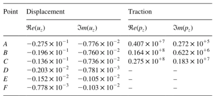
Table 1

Response forEfˆEs

Point Displacement Traction

R_e…uz† I_m…uz† R_e…pz† I_m…pz†

A 20:275£1021

20:776£1022 ₀

:407£1017 ₀

:272£1015

B 20:196£1021

20:760£1022 _0:164

£1018 _0:622

£1016

C 20:136£1021

20:736£1022 _0:275

£1018 _0:183

£1017

D 20:203£1022

20:781£1023 _{± ±}

E 20:152£1022

20:105£1022 _{± ±}

F 20:778£1023

20:103£1022 _{± ±}

Table 2

CPU times and number of iterations for solving the system…EfˆEs†

Solver CPU time (s) No. of iterations

Gauss elimination 0:206£1014 _±

Complex-J-BiCG 0:206£1013 ₁₀₄

schemes for symmetric matrices [26,27,32,39], satisfac-tory results in BEM analyses were obtained in the last ten years in applications of Lanczos-tridiagonalization-based iterative algorithms and generalised gradient methods by many researchers [20,22,32,35,38]. In this work, the only preconditioning matrixQused is the Jacobi splitting matrix, which is de®ned by the diagonal (complex-valued) of the system matrix.

4.3. The real version of the iterative scheme

An alternative procedure to iterative schemes for complex coef®cient matrices is naturally their correspond-ing real versions. For the complex system indicated in Eq. (7), for instance, simple complex arithmetic operations can be carried out, giving as a result the following real equivalent system:

Re…A† 2Im…A†

I_m…A† R_e…A†

" # _R

e…x†

I_m…x†

( )

ˆ

Re…b†

I_m…b†

( )

: …28†

As the system in Eq. (28) is real, the usual solvers for real matrices can be applied. However, better results were obtained here by using the following diagonal precondition-ing matrixQ:

qiiˆmax‰Re…aii†;Im…aii†Š …29†

4.4. Termination criterion

In order to terminate the iterative procedure for matrices with complex coef®cients, the following criterion was adopted: the Euclidian norm of the real and imaginary parts of the residue vector at the current iteration, say

iR_e…rn_†iandiI_m…rn_†i;were calculated and compared with a certain tolerancez(a real positive number); whenever the norm of both parts were smaller than a ®xed tolerance, the

iterative procedure was terminated. One has therefore:

if

iR_e…rn_†i,z

and then stop

iI_mrn†i,z

8 > > <

> > :

: …30†

For the real versions of the algorithms, see Eq. (28), a criterion equivalent to that given by expression (30) is adopted, such that the ef®ciency of both versions of the iterative scheme (the complex and the real) can be correctly compared one to another. It should be observed that

iR_e…rn_†1I_m…rn_{†i,z could also have been used as a} termination criterion, however the criterion shown in expression (30) has been preferred in the present work.

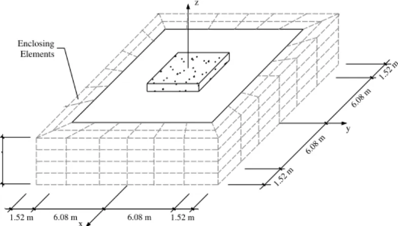
5. Applications

The soil-foundation interaction problem depicted in Fig. 3 is analysed in order to check the performance of the coupling algorithm proposed. The problem is modelled with two sub-regions (one is the foundation and the other is the soil), such that the whole model contains 1303 nodes and 420 elements that corresponds to a complex-valued coupled system of 3909 equations (Fig. 4).

The soil parameters areEsˆ2:0£108Nm22;nsˆ0:35

and rsˆ1800 Kg m23: nf ˆ0:25 and rf ˆ2500 Kg m23

were adopted for the foundation and four different values were adopted for its elasticity modulus: E_f ˆE_s; E_f ˆ

10E_s; E_f ˆ20E_s andE_f ˆ40E_s:

The square foundation side length and height are 1:52 and 0:19 m; respectively: The excitation loading considered was a harmonic distributed load of amplitude 4:0_£ 106Nm22_{and frequency 100 rad s}21 _{acting on the vertical}

direction at the top surface of the foundation. The results of the analysis in terms of displacements, tractions, CPU times F.C. ArauÂjo et al. / Engineering Analysis with Boundary Elements 25 (2001) 795±803

Table 3

Response forEfˆ10Es

Point Displacement Traction

R_e…uz† I_m…uz† R_e…pz† I_m…pz†

A 20:255£1021

20:744£1022 ₀

:368£1017

20:181£1015

B 20:202£1021

20:746£1022 _0:273

£1018 _0:822

£1016

C 20:151£1021

20:742£1022 _0:768

£1018 _0:622

£1017

D 20:190£1022

20:733£1023 _{± ±}

E 20:152£1022

20:103£1022 _{± ±}

F 20:807£1023

2103£1023 _{± ±}

Table 4

CPU times and number of iterations for solving the system…Efˆ10Es†

Solver CPU time (s) No. of iterations

Gauss elimination 0:206£1014 _±

Complex-J-BiCG 0:648£1013 ₃₂₈

Real-J-BiCG 0:119£1014 ₄₄₁

Table 5

Response for…Efˆ20Es†

Point Displacement Traction

R_e…uz† I_m…uz† R_e…pz† I_m…pz†

A 20:247£1021

20:742£1022 ₀

:341£1017

20:292£1015

B 20:204£1021

20:745£1022 _0:302

£1018 _0:685e

£1016

C 20:159£1021

20:744£1022 _0:981

£1018 _0:666

£1017

D 20:191£1022

20:728£1023 _{± ±}

E 20:155£1022

20:103£1022 _{± ±}

F 20:832£1023

20:104£1022 _{± ±}

Table 6

CPU times and number of iterations for solving the system…Efˆ20Es†

Solver CPU time (s) No. of iterations

Gauss elimination 0:206£1014 _±

Complex-J-BiCG 0:880£1013 ₄₄₅

and number of iterations are shown on Tables 1±8. The points considered for showing the response are de®ned as follows: A is the point at the interface centre, B is the midpoint of an interface edge,Cis the point at an interface corner, andD,E, andFare, respectively, soil points 1.0, 2.0 and 3.0 belowA.

The direct solver considered is the standard Gauss elim-ination procedure without any pivoting strategy and that takes into account the zero blocks of the coupled system. Complex-J-BiCG and the Real-J-BiCG stand for the complex and real equivalent versions of the biconjugate gradient procedure with Jacobi preconditioner, respectively. The termination criterion used for the iterative solver is that de®ned by Eq. (30), the tolerance being established by takingzˆ1025_{:The analyses were carried out in a personal}

computer with processor AMD K7 Ð 700 MHz and 640 Mbytes RAM, so that memory swapping (in/out-of-core transfer) was necessary.

6. Conclusions

The results presented in this paper show that the coupling algorithm developed, based on the use of iterative solvers, performs very well in what concerns response accuracy and convergence properties. No signi®cant differences was found between results obtained with iterative solvers and those obtained by means of a coupling algorithm based on a direct solver, thus only one response concerning tractions and displacements is presented on Tables 1, 3, 5, and 7. An important fact to be observed, concerning the iterative solver analyses, is that the number of iterations required to reach convergence increased when the relationship between the elasticity modulus of the foundation and the soil increased. Based on the data shown on Tables 2 and 8 for instance, one can see that the Complex-J-BiCG iterative

solver is, for Ef ˆEs; 10 times faster than the direct one

(standard Gauss), and forE_f ˆ40E_s;only 1.8 times faster than that solver, the corresponding Real-J-BiCG solver being initially (for E_f ˆE_s† six times faster and ®nally (for E_f ˆ40E_s† even a little bit slower than the standard Gauss direct solver. This fact should not be considered as a drawback of the iterative solvers algorithms, rather it just hints that when E_f ˆ40E_s a ®ner mesh is required to describe accurately the problem solution. This does happen because tractions amplitudes near the foundation edges increase considerably as the relationship Ef/Es increases,

such that in order to better describe the tractions over the interface a ®ner mesh near the edges is required. It should be also noted, that the scaling factor de®ned by Eq. (9), plays an important role for accelerating the convergence rate of the iterative solvers whenEf/Esincreases.

Other advantages of the iterative-solver-based coupling strategy presented here are that the zero blocks of coef®-cients are completely disregarded during the solution phase. It is therefore expected for coupled systems of order much higher than that one treated here, that iterative-solver-based coupling algorithms perform much better than direct-solver-based coupling strategies. Storage area required and conse-quently swapping time of direct solvers may restrict their use in more complex applications.

Speci®cally for the frequency-dependent soil-foundation interaction problem treated here, the Complex-J-BiCG solver was more ef®cient than the direct one for all relation-ships Ef/Es considered, even though no pivoting strategy

was employed in the latter solver. Concerning the iterative procedures, the complex version was more ef®cient than the real one; note that the number of iterations necessary to reach the convergence with the real version of the iterative scheme is greater than that of the complex one in all cases, and so it is the CPU time as well. One should observe that the preconditioning matrices in both versions are not the same (see Eq. (29)), such that the preconditioned versions of the iterative solvers are actually not identical; the preconditioning matrix given by Eq. (29) had a better performance than that Jacobi preconditioning matrix de®ned in the usual way for the equiva-lent real system of equations given in Eq. (28).

Finally, it is important to mention that the results presented in this paper hint that the complex version of iterative solvers should be used instead of the real equiva-lent versions, yet more numerical experiments are necessary in order to verify if this is always the case.

References

[1] Cruse TA. The transient problem in classical Elastodynamics solved by integral equations. PhD thesis, University of Washington, 1967. [2] Papoulis A. A new method of inversion of Laplace transforms. Q

Appl Math 1957;14(4):405±14.

[3] Durbin F. Numerical inversion of Laplace transforms: an ef®cient improvement to Dubner and Abate's method. Comp J 1974;17:371±6.

F.C. ArauÂjo et al. / Engineering Analysis with Boundary Elements 25 (2001) 795±803

Table 7

Response forEfˆ40Es

Point Displacement Traction

R_e…uz† I_m…uz† R_e…pz† I_m…pz†

A 20:239£1021

20:743£1022 ₀

:308£1017

20:347£1015

B 20:207£1021

20:746£1022 _0:326

£1018 _0:556

£1016

C 20:169£1021

20:748£1022 _0:124

£1019 _0:664

£1017

D 20:194£1022

20:728£1023 _{± ±}

E 20:159£1022

20:104£1022 _{± ±}

F 20:863£1023

20:105£1022 _{± ±}

Table 8

CPU times and number of iterations for solving the system…Efˆ40Es†

Solver CPU time (s) No. of iterations

Gauss elimination 0:206£1014 _±

Complex-J-BiCG 0:116£1014 ₅₈₈

[4] Manolis GD. Dynamic response of underground structures. PhD thesis, University of Minnesota, 1980.

[5] Manolis GD. A comparative study on three boundary element method approaches to problems in elastodynamics. Int J Num Meth Engng 1983;19:73±91.

[6] Mansur WJ, A time-stepping technique to solve wave propagation problems using the boundary element method. PhD thesis, University of Southampton, 1983.

[7] ArauÂjo FC. Time-domain solution of three-dimensional linear problems of elastodynamics by means of a BE/FE coupling process (in German). PhD thesis, Technical University of Braunschweig, Germany, 1994.

[8] Beskos DE. Boundary element methods in dynamic analysis. Appl Mech Rev 1987;40:1±23.

[9] Beskos DE. Boundary element methods in dynamic analysis: part II (1986±1996). Appl Mech Rev 1997;50:149±97.

[10] Wolf JP. Dynamic soil-structure interaction. Englewood Cliffs, NJ: Prentice-Hall, 1985.

[11] ArauÂjo FC, Mansur WJ, Nishikava LK. Determination of 3D time domain responses in layered media by using a coupled BE/FE process. In: Kassab A, Brebbia CA, Chopra M, editors. Boundary elements XX, Orlando, Florida, USA, Southampton: Computational Mechanics Publications, 1998. p. 587±96.

[12] Kane JH. Boundary element analysis in engineering continuum mechanics. Englewood Cliffs, NJ: Prentice-Hall, 1992.

[13] Banerjee PK. The boundary element method in engineering. New York: McGraw-Hill, 1994.

[14] Das PC. A disc based block elimination technique used for the solu-tion of non-symmetrical fully populated matrix systems encountered in the boundary element method. In: Proceedings of International Symposium on Recent Developments in Boundary Element Methods. Southampton, UK, 1978;391±414.

[15] Crotty JM. A block equation solver for large unsymetric matrices arising in the boundary element method. Int J Num Meth Engng 1982;18:997±1017.

[16] Kane JH, Kumar BL, Saigal S. An arbitrary condensing, non-condensing solution strategy for large scale, multi-zone boundary element analysis. Comput Meth Appl Mech Engng 1990;79:219±44. [17] Rigby RH, Alliabadi MH. Out-of-core solver for large, multi-zone boundary element matrices. Int J Num Meth Engng 1995;38:1507± 33.

[18] Bialecki RA, Merkel M, Mews H, Kuhn G. In- and out-of-core BEM equation solver with parallel and non-linear options. Int J Num Meth Engng 1996;39:4215±42.

[19] Ganguly S, Layton JB, Balakrishna C, Kane JH. A fully symmetric multi-zone Galerkin boundary element method. Int J Num Meth Engng 1999;44:991±1009.

[20] ArauÂjo FC, Mansur WJ. Boundary elements XI, Cambridge, USA, Southampton: Computational Mechanics Publications, 1989. p. 263± 74.

[21] ArauÂjo FC, Mansur WJ, Malaghini JEB. Biconjugate gradient accel-eration for large BEM systems of equations. Boundary elements XII,

Sapporo, Japan, Southampton: Computational Mechanics Publica-tions, 1990. p. 99±110.

[22] Mansur WJ, ArauÂjo FC, Malaghini JEB. Solution of BEM systems of equations via iterative techniques. Int J Num Meth Engng 1992;33:1823±41.

[23] Barra LPS, Coutinho ALGA, Telles JCF, Mansur WJ. Multi-level hierarchical preconditioners for boundary element systems. Engng Anal Boundary Elements 1993;12:103±9.

[24] Mang H, Li H, Han G. A new method for evaluating singular integrals in stress analysis of solids by the direct BEM. Int J Num Meth Engng 1985;21:2071±98.

[25] Manolis GD, Beskos DE. Boundary element methods in elasto-dynamics. London: Unwin Hyman, 1988.

[26] Hageman LA, Young DM. Applied iterative methods. New York: Academic Press, 1981.

[27] Hackbusch W. Iterative LoÈsung Grosser Schwachbesetzter Gleichungssysteme, B.G., Teubner Stuttgart, 1991.

[28] Doblare M. Three-dimensional formulation of the boundary element method with parabolic interpolation (in Spanish). PhD thesis, Poly-technical University of Madrid, Spain, 1981.

[29] Bettess JA. Economical solution technique for boundary integral matrices. Int J Num Meth Engng 1985;19:1073±7.

[30] Parreira P. Error analysis in the boundary element method in elasticity (in Portuguese). PhD Thesis, Technical University of Lisboa, Portugal, 1987.

[31] Mullen R, Rencis JJ. Iterative methods for solving boundary element equations. Comput Struct 1987;25:713±23.

[32] ArauÂjo FC. Iterative techniques for solving linear systems of equa-tions originated from the boundary element method (in Portuguese). MSc thesis, COPPE Ð Federal University of Rio de Janeiro, Brazil, 1989.

[33] Young DM, Hayes LJ, Jea KC. Generalized conjugate gradient accel-eration of iterative methods, Part I and II. Research Report CNA 162 and CNA 163, Center for Numerical Analysis, University of Texas at Austin, 1980.

[34] Young DM, Jea KC. Generalized conjugate gradient acceleration of nonsymmetrizable iterative methods. Linear Algebra Appl 1980;34:159±94.

[35] Barra LPS, Coutinho ALGA, Mansur WJ, Telles JCF. Iterative solu-tion of BEM equasolu-tions by GMRES algorithm. Comput Struct 1992;44:1249±53.

[36] Wilkinson JH. The algebraic eingenvalue problem. Oxford: Claredon Press, 1965.

[37] Fletcher R. Conjugate gradient methods for inde®nite systems, Lecture notes in mathematics 506. Berlin: Springer, 1976. [38] Prasad KG, Kane JH, Keyes DE, Balakrishna C. Preconditioned

Krylov solvers for BEA. Int J Num Meth Engng 1994;37:1651±72. [39] Axelsson O, Barker VA. Finite element solution of boundary value

problems Ð theory and computation. New York: Academic Press, 1984.