Rodolfo Telo Martins de Abreu

(1)

Rodolfo Telo Martins de Abreu

Licenciatura em Ciências de Engenharia Biomédica

Algorithms for Information Extraction and

Signal Annotation on long-term Biosignals

using Clustering Techniques

Dissertação para obtenção do Grau de Mestre em Engenharia Biomédica

Orientador: Prof. Doutor Hugo Filipe Silveira Gamboa

Júri:

Presidente: Prof. Doutor Mário António Basto Forjaz Secca Vogais: Profa. Doutora Valentina Borissovna Vassilenko

Prof. Doutor Hugo Filipe Silveira Gamboa

(2)

(3)

iii

Algorithms for Information Extraction and Signal Annotation on long-term Biosignals using Clustering Techniques

Copyright c Rodolfo Telo Martins de Abreu, Faculdade de Ciências e Tecnologia, Uni-versidade Nova de Lisboa

(4)

(5)

Acknowledgements

This dissertation, along with the conclusion of this course of studies, represents a crucial step in my life in which many people deserve my sincere gratitude.

First, I am sincerely grateful to my advisor, Prof. Hugo Gamboa for all the support and shared expertise that greatly contributed in achieving the purposed objectives for this dissertation. I also thank the given opportunity to work in such a healthy business environment, allowing me to grow and evolve personally and professionally.

I would like to thankPLUX - Wireless Biosignals, S.A.and all of its team members for creating a healthy environment where moments of hard work and pure entertainment were reconciled harmoniously. Then, I thank Neuza Nunes, Nídia Batista, Lídia Fortu-nato, Nuno Cardoso and Tiago Araújo. I also owe a special thanks to Joana Sousa for all the support under various circumstances and for always having the right word when I most needed. Finally, also a special thanks goes to my thesis’ colleagues Ricardo Chorão, Diliana Santos, Angela Pimentel and Nuno Costa for all the support, laughs and lunches that we shared over these last months.

To my friends Cátia, Mafalda, Margarida, Teresa Gabriel, Sofia, Ricardo, Teresa Neves, Ana and Filipa for making these last five years unforgettable. A very special thanks to my long-time friends Catarina, Ana, Marcos José, Marcos André and Patrícia for supporting me from the beginning (almost literally).

(6)

(7)

Abstract

One of the biggest challenges when analysing data is to extract information from it, especially if we dealing with very large sized data, which brings a new set of barriers to be overcome. The extracted information can be used to aid physicians in their diagnosis since biosignals often carry vital information on the subjects.

In this research work, we present a signal-independent algorithm with two main goals: perform events detection in biosignals and, with those events, extract informa-tion using a set of distance measures which will be used as input to a parallel version of thek-means clustering algorithm. The first goal is achieved by using two different ap-proaches. Events can be found based on peaks detection through an adaptive threshold defined as the signal’s root mean square (RMS) or by morphological analysis through the computation of the signal’smeanwave. The final goal is achieved by dividing the dis-tance measures intonparts and by performingk-means individually. In order to improve

speed performance, parallel computing techniques were applied.

For this study, a set of different types of signals was acquired and annotated by our algorithm. By visual inspection, theL1andL2 Minkowski distances returned an output

that allowed clustering signals’ cycles with an efficiency of 97.5% and 97.3%, respec-tively. Using themeanwavedistance, our algorithm achieved an accuracy of97.4%. For the downloaded ECGs from the Physionet databases, the developed algorithm detected 638 out of 644 manually annotated events provided by physicians.

The fact that this algorithm can be applied to long-term raw biosignals and without requiring any prior information about them makes it an important contribution in biosig-nals’ information extraction and annotation.

Keywords: Biosignals, Waves, Events detection, Features extraction, Pattern recognition,

(8)

(9)

Resumo

Um dos maiores desafios quando se estão a analisar dados é a capacidade de extrair informação dos mesmos, principalmente se estivermos a lidar com dados de grandes dimensões, o que traz um novo conjunto de barreiras a serem ultrapassadas.

Neste trabalho de investigação, é apresentado um algoritmo independente do tipo de biosinal que estiver a ser analisado e que apresenta dois objectivos principais: o primeiro prende-se com a detecção de eventos. Posteriormente, são retiradas medidas de distância que irão ser colocadas comoinputnuma nova versão paralela do algoritmo declustering k-means. A aplicação de técnicas declusteringirá permitir a extração de informação

rele-vante dos sinais.

O primeiro objectivo é concretizado recorrendo a duas abordagens distintas. Numa vertente mais simples e computacionalmente mais leve, os eventos podem ser detectados através da computação dos picos do sinal, onde o limiar é adaptável e definido como o valor quadrático médio do sinal; por outro lado, a detecção de eventos pode resultar de uma análise morfológica e da computação da onda média representativa do sinal. O último objectivo é concretizado dividindo as medidas de distância previamente obtidas emnpartes e aplicando o algoritmo k-means em cada uma delas individualmente. De

modo a diminuir o tempo de processamento foram utilizadas técnicas de programação em paralelo.

Para este estudo foram adquiridos e anotados pelo nosso algoritmo diversos tipos de sinais. De modo a realizar a validação do algoritmo, recorreu-se a uma inspecção visual dos sinais processados, obtendo-se uma eficiência de97.5% e de97.3% quando utilizadas as distâncias de MinkowskiL1eL2, respectivamente. Utilizando a distância à

onda média, o nosso algoritmo atingiu uma precisão de97.4%. Relativamente aos ECGs que foram obtidos nas bases de dados daPhysionet, o algoritmo desenvolvido conseguiu

detectar 638 das 644 anotações clinicamente relevantes fornecidas por médicos.

O facto do algoritmo desenvolvido poder ser aplicado em sinais raw, de longa

(10)

x

represente uma importante contribuição na área do processamento de sinal e, mais espe-cificamente, na anotação e extracção de informação de biosinais.

(11)

List of Figures

1.1 Thesis overview . . . 2

2.1 Biosignal’s types and classification. Adapted from [1]. . . 6

2.2 General block diagram for the aquisition of a digital signal. Adapted from [1, 2]. . . 7

2.3 Electrophysiology of the heart. From [3].. . . 10

2.4 Surface EMG recording. Adapted from [4]. . . 11

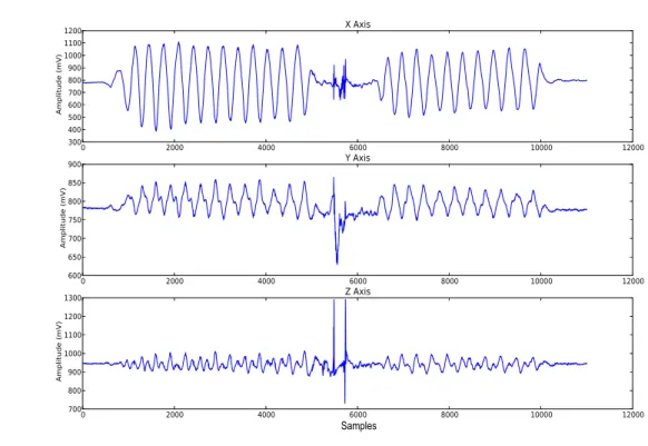
2.5 Acceleration signals acquired with a three axis sensor. . . 12

2.6 Example of a BVP signal with annotations of the main points in one cycle. 13 2.7 (a) Highlight of an ECG signal with the R-peaks annotated and (b) the computed ECG envelope allowing the estimation of the respiratory signal. 14 2.8 General procedure of supervised learning.. . . 15

2.9 Basic process for cluster analysis. From [5, 6]. . . 17

3.1 Peaks detections using the RMS of the signal as an adaptive threshold. The horizontal lines represent the evolution of the threshold over time. . . 24

3.2 Signal Processing Algorithm Steps. . . 25

3.3 Autocorrelation function of a cyclic signal. . . 27

3.4 (a) Highlight of event alignment using a meanwaveand a wave reference point; Events alignment in an ECG signal using (b) themeanwaveand (c) the wave reference points. . . 29

3.5 Waves and meanwavealignment and construction using (a)meanwave ref-erence point and (b) waves refref-erence points.. . . 30

3.6 (a) Distance matrix for an ECG signal and (b) the highlight of the first30_× 30elements of the distance matrix. . . 32

3.7 Parallelk-means algorithm schematics.. . . 34

(14)

xiv LIST OF FIGURES

4.1 Clustered synthetic signal with four different modes and with no changes in the fundamental frequency. . . 39 4.2 bioPluxResearch system. . . 40 4.3 Clustering using events time-samples variability. A clear transition

be-tween the rest and the exercise state of the subject is annotated using this information. . . 42 4.4 Highlight of an annotated ECG signal where the noise area (green dots) is

indicated as different from the remaining areas of the represented signal (red dots). . . 44

5.1 wiCardioRespProject schematics. From [7]. . . 52 5.2 Highlight of an ECG signal recorded from a patient diagnosed with CAD.

(15)

List of Tables

4.1 Results concerning the developed events detection algorithm on synthetic signals. . . 38 4.2 Clustering results on synthetic signals. The value ofkrepresents the

num-ber of modes present in the signal and also the numnum-ber of clusters. . . 38 4.3 Clustering results using∆iwithk= 2clusters . . . 43

4.4 Clustering results using morphological comparison withk= 2clusters. . 47 4.5 Clustering results using morphological comparison with kclusters

(con-tinuation). . . 48 4.6 Accuracy obtained using different distance functions to obtain inputs for

the clustering algorithm. . . 48 4.7 Clustering results for the ECG signals downloaded from the Physionet

databases. . . 49

(16)

(17)

Acronyms

AAL Ambient Assisted Living

ACC Accelerometry

ADC Analog-to-Digital Converter

ADL Activities of Daily Livings

AHD Atherosclerotic Heart Disease

AI Artificial Intelligence

AmI Ambient Intelligence

BVP Blood Volume Pressure

CAD Coronary Heart Disease

CNS Central Nervous System

ECG Electrocardiography

EEG Electroencephalography

EMG Electromyography

FFT Fast Fourier Transform

HR Heart Rate

HRV Heart Rate Variability

IC Inspiratory Capacity

LED Light-Emitting Diode

(18)

xviii ACRONYMS

RMS Root Mean Square

RV Residual Volume

SNR Signal-to-Noise Ratio

TLC Total Lung Capacity

TV Tidal Volume

(19)

1

Introduction

1.1 Motivation

One of the biggest challenges nowadays is to increase people’s life expectancy while reaching those late ages with a high quality of life, living independently for a longer period of time. Although technology is constantly evolving, these goals could not be reached if a closer and regular monitoring of patients was not taken. Thus, the inevitable increase of data to be analyse becomes a concern for physicians and technicians due to the exhaustive and time-consuming nature of this type of tasks.

The search and development of computer-aid techniques to automatically analyse data is continuously growing. In the signal processing field, these tools are usually de-veloped to analyse only one type of signals, such as electrocardiography (ECG), elec-tromyography (EMG), respiration, accelerometry (ACC), among others. The main goal of these tools is to monitor activities and vital signs in order to detect emergency situ-ations or devisitu-ations from a normal medical pattern [8]. Besides, the barriers that arise when dealing with long records (provided by a continuous monitoring of ill patients at home, for example) are yet to be overcome.

(20)

1. INTRODUCTION 1.2. Objectives

This dissertation was developed at PLUX - Wireless Biosignals, S.A., under the Re-search and Development (R&D) department. One of the major goals of this department is to create innovative solutions for comfortably monitoring people under a variety of scenarios (at healthcare facilities, home, training facilities, among others). Besides, it also aims at developing signal processing tools for extracting information from the biosignals acquired during the people’s monitoring. The possibility to contribute with the devel-opment of signal processing tools and the given opportunity of working in a business environment strongly encouraged this research work.

1.2 Objectives

This thesis aims at the development of a signal-independent processing algorithm able to perform clustering techniques in long-term biosignals and extracting information from them. With that information, the output of the algorithm is an annotated signal. Due to the high level of abstraction present in our algorithm, a set of different types of biosignals was acquired to test its performance, including ECG, EMG, blood volume pressure (BVP), respiratory and ACC signals. An events detection tool was first implemented, distance measures were taken using different distance functions and a parallel version of thek

-means clustering algorithm was also designed and characterized.

Due to the suitability of our algorithm in long-term biosignals, parallel computing techniques were applied in order to improve performance.

1.3 Thesis Overview

In Figure1.1it is exposed the structure of the present thesis.

Appendix

Publications

Results / Discussion

4. Performance Evaluation 5. Applications 6. Conclusions

Methods / Tools

3. Signal Processing Algorithms

Preliminaries

1. Introduction 2. Theoretical Concepts

Figure 1.1: Thesis overview

(21)

1. INTRODUCTION 1.3. Thesis Overview

exposed and the main objectives are also briefly explained. In Chapter 2, a theoretical contextualization of the concepts used in this thesis is provided and a state of the art is also characterized. These two chapters comprise the thesis’s Preliminaries.

In Chapter3, the signal processing algorithms that were developed to fulfil the the-sis’s objectives are depicted. The two developed approaches to detect events on biosig-nals and the parallel version of thek-means clustering algorithm are exposed. This chap-ter accounts for the thesis’s Methods/Tools.

The last three chapters address the results and discussion of this research work. In Chapter 4, the procedures to test our algorithm performance are exposed, including the visual inspections and comparison with the annotated signals from the Physionet databases. In Chapter5some specific applications of our algorithm are presented, show-ing its applicability in this research topic. To conclude, an overview of the developed work, results and contributions are presented and some future work suggestions are dis-cussed in Chapter6.

The thesis writing was done using the LA_{TEX environment [}₉_{]. The signal processing}

(22)

(23)

2

Concepts

In this chapter the main concepts that were used in this dissertation are presented. Fun-damentals on biosignals, biosignal acquisition, biosignal processing and machine learn-ing will be stated.

2.1 Biosignals

Biosignals can be described as space-time records of biological events that generate phys-iological activities (e.g. chemical, electrical or mechanical) —biological signals— likely to

be measured [2,11].

2.1.1 Biosignals Classification

Biosignals are usually divided according to the physiological phenomenon that was be-hind their generation. Thus, the most current and important classifications are [2,12]:

• Bioeletric (Electrophysiologic) Signals: When a stimulus is enough to depolarize a cell’s membrane, an action potential is generated which leads to electrical changes that can be measured by electrodes. Electrocardiogram, electromyogram or elec-troencephalogram are examples of bioelectric signals.

• Biomechanical Signals: These signals are associated with biological motion that generates force, such as blood pressure.

(24)

2. CONCEPTS 2.1. Biosignals

SIGNALCLASSES

Continuous Discrete

SIGNALGROUPS

Deterministic Periodic (signal waveshape is repeated periodically) Nonperiodic (signal waveshape

is not repeated periodically)

Quasi-Periodic

(signal waveshape is repeated almost

periodically) Transient (waveshape occurs only once) Stochastic Stationary (statistical properties do not

change in time)

Nonstationary (statistical properties change

in time)

Figure 2.1: Biosignal’s types and classification. Adapted from [1].

• Biomagnetic Signals: Magnetic fields can be generated by the human body due to the electrical changes that occur within it. Magnetoencephalogram is an example of biomagnetic signals.

Biosignals can also be classified asdeterministicorstochastic. Deterministic signals can be described by mathematical functions or even by plots. Although most of the real-world signals are nondeterministic, it is quite usual to define a model (or function) that approximately describes the signal to be analysed.

One of the most important type of deterministic signals is theperiodic signals, that

are characterized by a time intervalT that separates two successive copies of the signal. Thus, beingx(t)a periodic signal, it can be expressed as

x(t) =x(t+kT) (2.1)

where kis a integer. Although most of the real-world signals are nonperiodic, there is a very important class —quasi-periodic signals— which includes signals that have some slight changes along their cycles, so they can be considered as almost periodic. It is the example of the ECG signal; in fact, the time between R peaks is always different but approximately equal, and so ECG’s PQRST complex interval of one heart beat is almost the same as the next.

(25)

Sensor Amplifier Analog_Filter Sampler Quantizer _StorageData _ProcessingDigital

Analog Signal–�(t) ADC Converter Digital Signal–�[�]

Figure 2.2: General block diagram for the aquisition of a digital signal. Adapted from [1,2].

It is also common to divide biosignals incontinuousanddiscrete. Continuous biosig-nals are described by functions that use continuous variables or by differential equations and can be represented mathematically byx(t), wheretis a continuous variable – time. Thus, continuous biosignals provide information at any instant of time. Most of the bio-logical signals are continuous in time, such as ECG, EMG, BVP, among others.

On the other hand, discrete biosignals (or time-series) are described by functions that use discrete variables, i.e. digital sampled data. This type of biological signals can be represented mathematically byx[n], wheren= 0, . . . , Lrepresents a subset of points of t, withLthe length of the signal. Therefore, discrete biosignals only provide information at a given discrete point along the time axis [1,2,13].

2.1.2 Biosignals Acquisition

Biosignals are collected using sensors that are able to convert certain biological activi-ties (e.g. heart beat, respiratory movements) into an electrical output. Since computers only have the capacity to store and process discrete amounts of information [14], it is necessary to convert the continuous data into discrete units in order to allow the pro-cessing. Besides, the most important developments in signal processing are related to discrete signals. Thus, it is common to convert a continuous signal into a discrete one using an Analog-to-Digital Converter (ADC). ADC is a computer controlled voltmeter that transforms continuous biological signals into digital sequences [1,2].

The transformation of the ADC comprises two steps:samplingandquantization. Math-ematically, the sampling process can be described as [1]:

x(t) =x(n)_|n=tTs (2.2)

(26)

Tsthe sampling interval. Thus, the sampling frequency,fs, can be defined as:

fs=

2π

Ts (2.3)

However, fs must verify an important condition in order to guarantee that the discrete

signal is no different (no information added or removed) from the original signal. This is very important in any area but since the result of biosignals processing might be used to assist physicians on diagnosis, this feature becomes even more essential [2]. In fact, being F the higher frequency present in the original signal, iffs = 2F it is said that the signal

is Nyquist-sampled andfsis called the Nyquist frequency [14]. Therefore, the Nyquist

theorem defines a minimal sampling frequency given by [15]:

fs >2F (2.4)

In the quantization process, each value of the signal amplitude can only assume a fi-nite number of values. This process is related to the ADC resolution which is the number of bits that are going to be used to generate a digital approximation. Thus, this process brings inherently loss of information, which can be attenuated by increasing the available number of bits [2,14].

2.1.3 Biosignals Processing

Biosignal processing is necessary in order to extract relevant information present in raw data. Although most of the processing techniques are applied in digitized signals, some analogue signal processing is usually necessary [16]. However, for the purpose of this dissertation, we will only focus on digital signal processing.

After the biosignal acquisition phase, the next step is to interpret the meaning of the acquired signal. To accomplish that, it is often necessary to apply different types of pro-cessing: pre-processingandspecialized processing[17].

Signal pre-processing can also be called as signal "enhancement" because it allows to separate the acquired information from the inherent noise that appears due to most of the measurement systems, which is a limiting factor in the performance of instruments. Besides, external factors such as movement during the acquisitions might also induce noise appearance. However, the acquisition conditions also influence the quality of the acquired signal.

Thus, the first signal processing techniques emerge due to the necessity of removing noise artefacts, which were limiting the extraction of useful results disguised by them. These techniques usually consist in the application of some specific filters that allow noise removal without eliminating signal’s (useful) information and improving, therefore, the

(27)

SN R= 20 log

_Signal

N oise

(2.5)

whereSignalrepresents the signal’s useful information andNoisethe signal’s noise [1,16, 17].

Once the pre-processing phase is finished, a specialized processing is applied to sig-nals, along with classification and recognition algorithms [17].

In general, it is only after the pre-processing and specialized processing steps that the result of the acquisition process reveals the true meaning of the physical phenomenon that produced the signal under analysis.

2.1.4 Biosignals Types

In this sub-section a brief description of electrocardiography, electromyography, accelerom-etry, blood volume pressure and respiratory signals (the main biosignals addressed in this research work) will be presented.

Electrocardiography

The electrocardiography (ECG) signal is one of the most well studied biosignals, because changes due to pathologies are easily detected and its acquisition process is quite simple. These factors contribute to its wide use in medicine [14].

Since every single muscle on the human body needs an electrical stimulus to contract or relax, the heart’s muscle — myocardium — is no exception. In fact, as we can see in Figure2.3(a), there is a group of cells located on the right atrium that are responsible to generate a depolarization wave (due to a certain stimulus). These cells are designated as the pacemaker cells and together form the sinoatrial (SA) node. Then, the bundle of His assures that the depolarization wave propagates along the heart, which results on the contraction of myocardium. All this process generates currents and, consequently, a measurable electrical signal [14,18].

As a result of the electrical conductivity of the human tissues, this electrical signal dis-perses all around the body, making it possible to be detected on the body surface. There-fore, the ECG wave form (Figure 2.3(b)) results from the sum of the electrical changes within the heart. The first portion is designated as P wave and is related to the atria de-polarization and the QRS complex is due to the ventricle dede-polarization. Then appear two more waves, T e U, assigned to the repolarization of ventricles and atria, respec-tively. Most of the times the U wave is masked by the ventricular depolarization of the following cardiac cycle [2,14,18].

(28)

(a) The origin of the electrical activity

P

Q R

S

T ST

Segment

PR Segment

PR Interval

QT Interval QRS

Complex

(b) Pattern of a normal ECG signal

Figure 2.3: Electrophysiology of the heart. From [3].

Electromyography

The electromyography (EMG) signals relate to the electrical signals that are behind mus-cle contraction. These signals can be recorded by electrodes inserted in the musmus-cle (in-tramuscular recordings) or located over the skin (surface recordings). Surface recordings are the most used method since they are non-invasive. In this research work, only the surface recording method was used in order to obtain this type of biosignals [14].

Just like it was mentioned before, every muscle needs an electrical stimulus to begin its activity. These signals are generated on nerve cells called motor neurons. A motor unit is defined as the joint of a motor neuron and all the muscles fibers that it innervates. When a motor unit becomes active, an electrical signal stimulates muscles to contract and this electrical signal corresponds to the resulting electromyographic signal [19,20]. Therefore, the time when a motor unit becomes active represents the EMG’s onset; like-wise, the time when a motor unit becomes inactive represents the EMG’s offset.

In Figure2.4the procedure to acquire EMG surface recordings is shown. When the EMG is acquired from electrodes mounted directly on the skin, the signal is a compos-ite of all the muscle fiber action potentials occurring in the muscles underlying the skin. Therefore, in order to obtain individual motor unit action potentials, a signal decompo-sition is required [1,4].

Since the EMG detects the electrical activity of muscles, it represents an important diagnostic tool in detecting muscle dysfunctions.

Accelerometry

(29)

Figure 2.4: Surface EMG recording. Adapted from [4].

velocity of an object. Therefore, its units arem/s2_or

gunits, where1g= 9.81m/s2_.

In order to measure the acceleration, accelerometers are used. Initially, accelerometers were designed only to be sensitive in one direction but nowadays, accelerometers are capable of measuring acceleration in each orthogonal axis [14]. However, the calibration process is quite important. In fact, the output of a stationary accelerometer pointing toward global vertical must be 1g(or−1g, depending the accelerometer’s orientation) [21].

Since an accelerometer is usually small and its utilization is inexpensive, it has been widely used in monitoring human motion and in classifying human movement patterns. Besides, it is quite important that movement measures are unobtrusive to obtain a more accurate monitoring of human motion [22,23].

Blood Volume Pressure

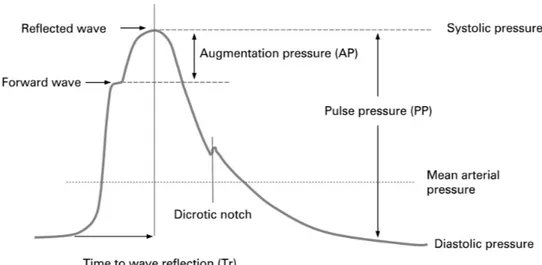
The peripheral pulse wave is a mechanical event closely following the ECG complex. It reflects the interplay between left ventricular output and the capacitance of the vascular tree [24].

(30)

Samples

Figure 2.5: Acceleration signals acquired with a three axis sensor.

By measuring the time between each cycle of the BVP signal, the heart rate (HR) can be computed and a heart rate variability (HRV) analysis can be undertaken.

This signal provides a method for determining properties of the vessels and changes with ageing and disease.

Despite the complex source of the signal and problems of measurement, this tech-nique has been widely used for the monitoring of arterial pressure, detecting anxiety, among other applications [27].

Respiration

Respiratory signals are directly or indirectly related to the lungs volume along each breath. The tidal volume (TV) is the amount of air flowing into and out of the lungs in each breath, which is typically 500 mL for an adult. However, the respiratory system has the ability to move much more air than the tidal volume. In fact, the inspiratory ca-pacity (IC) represents the maximum volume of air that someone can inhale. On the other hand, it is impossible to exhale all the lungs’ air and this volume represents the residual volume (RV). Finally, the total lung capacity (TLC) equals the vital capacity (VC) — the volume of air exhaled from a maximum inspiration to a maximum expiration — plus the residual volume [1,18].

(31)

2. CONCEPTS 2.2. Clustering

Figure 2.6: Example of a BVP signal with annotations of the main points in one cycle.

In fact, using a respiratory sensor which integrates a Piezo Film Technology (PVDF) sen-sor, changes in length related to the abdominal and thoracic movements can be measured, obtaining a respiratory signal where the respiratory cycles can be observed [28].

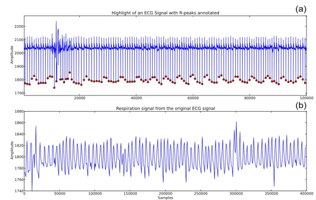
In Figure 2.7 an ECG and a respiratory signal are presented. Both signals are illus-trated in order to show the relationship between them. In fact, with the R-peaks detec-tion of an ECG signal, it is possible to estimate the correspondent respiratory signal, by computing the ECG envelope.

2.2 Clustering

2.2.1 Machine Learning and Learning Methods

Machine learningis a mechanism where due to the input of new data, computers (or ma-chines) change their structure or program in a way that is expected an improvement on future performance [29]. Therefore, machine learning is related toArtificial Intelligence

(AI), although most of the AI research does not concern with learning which make com-puters develop a task always the same way over time [30]. Google is an example where machine learning is a key feature [31]. In fact, when someone does a search, the input is classified and a set of pages that have the same classification are returned. Amazon [32] and any gaming company that have AI in their games also use machine learning.

(32)

(a)

(b)

Figure 2.7: (a) Highlight of an ECG signal with the R-peaks annotated and (b) the com-puted ECG envelope allowing the estimation of the respiratory signal.

The performance improvement over time requires that humans establish a set of rules for computers to use them to learn along with the new incoming data. Therefore, one of the main goals of machine learning is to generate classifications on input data simple enough to be understood by humans [34]. However, computers are not always capable of making the right decision (classification) when applying those rules; in fact, there is always an error and the main goal of the learning process is to minimize that error which is usually expressed by a function –error function. This leads to a new world called opti-mization[29].

As it was previously mentioned, one important aspect of machine learning is data classification. In fact, one of the most important tasks when analysing data is trying to find patterns or relationships in data in order to group it into a set of categories [5].

To accomplish that, two types of classification are used: thesupervised learningor the unsupervised learning, which is also known asclustering.

In the supervised learning approach, the learner (usually, the computer) receives in-put data,D, that will be divided into two sets: thetraining set,P_{, and the}

(33)

Figure 2.8: General procedure of supervised learning.

functionf between the labelled data and its output. Analogously, the testing set con-tains data that will be classified due to the previous learning process (represented by the functionf); if the obtained classifier is ideal, there will be no errors, which means thatf perfectly describes the entire data (training set plus testing set) [29,35]. Thus, the main objective in supervised learning is to label new data according to the previous labelled data received as input [36] and, as a result, data will be grouped into specific classes. In other words, it allows pattern recognition and this is why supervised learning is broadly used, despite its human and computational costs and limitations [37].

In opposition with the supervised learning, the unsupervised learning approach does not have a training set, which means that the learner only receives unlabelled data with no information about the class of each sample [37]. Therefore, the main goal of clustering is to separate data into a finite number of data structures using only the data itself [6,36]. These structures have to be organized in such a way that the intra-group variability is minimized and the inter-group dissimilarity is maximized [38]. It is worth noticing that clustering algorithms can be applied on raw data, although it is common to pre-process it [39].

2.2.2 Clustering Methods

In order to implement a clustering algorithm, it is necessary to define two major issues: in which way data objects are grouped and what’s the criteria to be used in the grouping process [40]. Therefore, according to the chosen grouping process, clustering algorithms can be broadly divided into five categories, which will be briefly described [5,6,36,38, 39,41]:

1. Partitioning Methods. These methods (or algorithms) separate data intok

(34)

algorithms are always designed according to an objective function and work well on spherical-shaped clusters and on small to medium data set. The well-known partition-based algorithms are thek-means andfuzzy c-means [42].

2. Hierarchical Methods. These methods group data objects into a tree of clusters (which can be also called a dendrogram) where the root node represents the whole data set, the leaf node a single object and the intermediate nodes represent how similar objects are from each other. Hierarchical algorithms can be broadly divided inagglomerativeanddivisivealgorithms. In agglomerative algorithms, each data ob-ject represents a cluster (singleton) and then the clusters are merged (according to their similarity) until a stop condition is achieved (if not, all the data objects will be-long to the same group), which usually is related to the number of desired clusters – bottom up approach. On the other hand, in divisive algorithms, all the data ob-jects represent one cluster and they are sliced into a specified number of clusters (if not, each data object will represent a single cluster) – top down approach. Most of the hierarchical clustering algorithms are variants of the single-link, complete-link or minimum-variance algorithms. CURE [43], BIRCH [44] and Chameleon [45] are examples of hierarchical algorithms.

3. Density-Based Methods.These algorithms are based on density in the neighbour-hood of a certain cluster: until that density exceeds a certain threshold, the cluster grows continuously. DBSCAN [46] and OPTICS [47] are examples of density-based algorithms.

4. Grid-Based Methods.These methods quantize the object space into a finite number of cells that form a grid structure on which all of the operations for clustering are performed, allowing a small processing time. STING [48] is an example.

5. Model-Based Methods. These methods divide data objects into clusters accord-ing to a specific model established for each cluster and it can be obtained usaccord-ing a statistical approach or a neural network approach.

2.2.3 Clustering Steps

Regardless of the various methods of clustering presented in the previous sub-section, cluster analysis can be divided into four major stages [5,6,36]:

(35)

Data Samples Feature Selection _{or Extraction} Algorithm Desing Clustering

or Selection

Cluster Validation Results

Interpretation Knowledge

Figure 2.9: Basic process for cluster analysis. From [5,6].

2. Clustering algorithm design or selection.Almost all clustering algorithms are con-nected to some particular definition of distance measure. Therefore, clustering algo-rithm design usually consists of determining an adequate proximity measure along with the construction of a criterion function, affecting the way that data objects are grouped within clusters.

3. Cluster Validation.When comparing different approaches, it is common to obtain different results (clusters); besides, when comparing the same algorithm, a change in pattern identification or presentation order of input patterns may result in dif-ferent clusters also. Thus, in order to accurately use clustering algorithms results, a cluster validation is necessary. This validation process must be objective and have no preferences to any algorithm but there is not an optimal (and general) procedure for clusters validation, except in well-prescribed subdomains.

4. Results interpretation. The main objective of clustering is to provide users infor-mation about the original data in order to solve the encountered problems. Since cluster results only represent a possible output, further analysis (e.g. using super-vised learning techniques) are necessary to guarantee the reliability of results.

2.2.4 Thek-means clustering algorithm

Thek-means clustering algorithm [49,50] is the best-known squared error-based

cluster-ing algorithm. In fact, this algorithm seeks an optimal partition of the data by minimizcluster-ing the sum-of-squared-error criterion. If we have a set of objectsx_j, _j _{= 1}_{, . . . , N}, and we

want to organize them intokpartitionsC =_{C1, . . . , Ck}, then the squared error criterion

is defined by [6,51]:

J(M_{) =}

k

X

i=1

N

X

j=1

||x_j₋m_i_||2 (2.6)

wherem_iis an element of the cluster prototype or centroid matrixM.

(36)

belongs to the category of the hill-climbing algorithms. The basic steps of this clustering algorithm are summarized as follows [5,38].

1. Initialize ak-partition randomly or based on some prior knowledge. Calculate the

cluster prototype matrixM_{= [}m₁_{, . . . ,}m_k_].

2. Assign each object,x_j, of the data set to the nearest cluster partition_C₌_{_C₁_{, . . . , C}_k_}

based on the criterion,

x_j _∈_C_w_, if_||x_j₋m_w_||_<_||x_j ₋m_i_|| (2.7)

forj= 1, . . . , N,i₆=wandi= 1, . . . , k.

3. Recalculate the cluster prototype matrix where each element will now be given by

m_i ₌ 1

Ni

X

xj∈Ci

x_j (2.8)

4. Repeat steps 2)-3) until there is no change in each cluster or, in other words, in the cluster prototype matrix’s elements.

In spite of its simplicity, easy implementation and relatively low time complexity, there are some major and well-known drawbacks, resulting in a large number of vari-ants of the originalk-means algorithm in order to overcome these obstacles. The major disadvantages are presented bellow [5,6].

• There is no automatic method to identify the optimal number of partitions, which must be given as an input for thek-means algorithm.

• The random selection of the initial partition to initialize the optimization procedure affects the centroids convergence, returning different results for the same data.

• The iteratively optimal procedure of k-means cannot guarantee convergence to a global optimum.

• The sensitivity to outliers and noise distorts the cluster shapes. In fact, even if an observation is quite far away from a cluster centroid, the k-means forces that observation into a cluster.

• The mathematical definitions adjacent to thek-means algorithm limits its

applica-tions only to numerical data.

(37)

2. CONCEPTS 2.3. Ambient Assisted Living

2.3 Ambient Assisted Living

One of the main objectives of this research work is to apply the developed algorithm to Ambient Assisted Living. Therefore, in this section a brief description of what is Ambient Assisted Living, along with its objectives and relevance will be presented.

Ambient Assisted Living (AAL) belongs to a larger definition of assisting users in their activities called Ambient Intelligence (AmI). AmI is basically a digital environment designed to assist people in their daily lives without interfering with them [52,53].

Through the use of wearable sensors, AAL aims at monitoring elderly and chroni-cally ill patients at their homes. Therefore, one of the main goals of AAL is to develop technologies which enable users to live independently for a longer period of time, in-creasing their autonomy and confidence in accomplishing some daily tasks (known as ADL, Activities of Daily Livings) [54,55].

Thus, AAL systems are used to classify a large variety of situations such as falls, phys-ical immobility, study of human behaviour and others. These systems are developed using an Ubiquitous Computing approach [56] (where sensors and signals processing are executed without interfering on ADL) and must monitor activities and vital signs in order to detect emergency situations or deviations from a normal medical pattern [8]. Ul-timately, AAL solutions automate this monitoring by using software capable of detecting those deviations.

2.4 State of the Art

Due to the constant evolution in sensing systems and computational power, biosignals acquisition and processing are always adapting to new technologies.

The main goal of clustering algorithms is to find information in data objects that al-lows to find subsets of interest — clusters — where objects in the same cluster have a maximum homogeneity. Therefore, the clustering base problem appears in various do-mains and is old, being traced back to Aristotle [51].

In fact, clustering algorithms can be typically applied to computer sciences, life and medical sciences, astronomy, social sciences, economics and engineering [5]. Due to these applications and area of research work, state-of-the-art developments in biosignals clus-tering and in Ambient Assisted Living (AAL) will be presented.

Applying clustering techniques to biosignals is an approach that has been used re-cently. Due to the large amount of data that is analysed nowadays, clustering techniques are used for feature extraction and pattern recognition on biosignals.

(38)

2. CONCEPTS 2.4. State of the Art

beats) into clusters that represent central features of the data. Lagerholm et al. (2000) [57] used a self-organizing network to perform beat clustering and detect different heart beats types. However, it was not made a heart rate variability analysis which could lead to a better detection of heartbeat types. On the other hand, Cuesta-Frau et al. (2002) [58] follow the previous approach but, after that, selected one single beat to represent all the beats in a cluster, allowing an automatic feature extraction of a long-term ECG. Since this approach requires a dissimilarity measure (measuring distances between arrays with dif-ferent lengths) to obtain an input to the clustering algorithm, it has an extremely high computational cost. Similarly, Ceylan et al. (2009) [59] used a Type-2 fuzzy c-means

(T2FCM) to improve the performance of a neural network, where T2FCM pre-classifies heart beats into clusters and a neural network is trained with the output of T2FCM, re-ducing also the training period. However, Chao et al. (2011) [60] usedc-medoidsto obtain

optimal ECG templates that would be further used to train a classifier able to separate ECG signals from other types of biosignals. Thus, this work can only identify ECG sig-nals and since there are more than 19 categories for these biosigsig-nals, in order to obtain a high accuracy it would require the construction of the templates of all categories.

Concerning clustering on EMG signals, Chan et. al (2000) [61] presented a classifier that was used to control prosthetics. However, in order to obtain high training speed, data features were clustered using the Basica Isodata algorithm and then fed to a back-propagation algorithm which input was used to determine which function would be exe-cuted by the prosthesis. Therefore, the delay between the onset of the EMG and the pros-thesis control was reduced (estimated to be 300 ms) but this control resulted in a limited number (four) of movements. Also, Ajiboye et al. (2005) [62] presented an heuristic fuzzy logic approach to classify multiple EMG signals for multifunctional prosthesis control. In this study, thefuzzy c-means clustering algorithm was used to automate the construction of a simple amplitude-driven inference rule base, which is common when using a heuris-tic approach to solve a certain problem. The usage of simple inference rules allows a short delay (45.7 ms) but this algorithm only allows the control of one degree-of-freedom at a time, which limits the prosthesis in performing combined movements.

Due to the increasing amounts of data coming from all types of measurements and observations, some parallel computing techniques have been applied to clustering algo-rithms. These parallel techniques usually consist in performingdata paralleland/ortask parallelstrategies. In the first strategy, the idea is to divide and distribute data into

(39)

Since one of this research work applications is the Ambient Assisted Living, a set of interesting projects and studies will be presented next.

AAL aims at developing technologies that allow elderly people and chronically ill patients living in their home environment for a long period of time by assisting them in accomplishing their activities independently [68].

To accomplish AAL goals, a large number of projects were developed. In fact, the Aware Home [69], I-Living [70] and Amigo [71] projects are based on building intelligent environments (also called smart houses) where a software infrastructure allows electronic equipments to work together, providing a set of centred services that assist elderly peo-ple and chronically ill patients. However, the social component of this environments is usually undervalued and the COPLINTHO project [72] tries to solve this failure [54]. Un-like the aforementioned projects, AAL4ALL also develops services and technologies to assist AAL users and it has the goal to enter in the business market and commercialize their products [56].

Along with AAL projects, there is some recent studies that contributed to AAL objec-tives. In fact, Steinhage et al. (2008) [73] created a sensor network embedded on the floor where feet pressure generates events that allowed fall detection and elderly people’s ac-tivity monitoring. Thus, users do not need to wear sensors embedded on cloths or be monitored by cameras, compromising their privacy, but the collected data has a high complexity and the installation costs of the system are quite high. On the other hand, Goshorn et al. (2008) [55] implemented a classifier capable of recognizing hand gestures, which generated commands for AAL communications, improving the recognition rates and increasing the available vocabulary since the set of hand gestures is based on the alphabet of anatomic hand postures. Since this approach is a supervised one, a limited number of hand gestures will be recognized. Besides, elderly people or chronically ill pa-tients performing correct and stable hand gestures can represent a difficult task for them.

(40)

to detect diseases or emergency situations on elderly people.

In fall detection domain, Luštrek et al. [76] developed a system where users wear accelerometers along with location sensors, allowing fall detection with contextual infor-mation. In this study, a variety of approaches were used, including unsupervised ones. However, in this study, it is necessary that subjects use many sensors in order to gather the required information, which can fail in reaching an ubiquitous approach, essential when performing human activity monitoring.

(41)

3

Signal Processing Algorithms

In this chapter the implemented signal processing algorithms are thoroughly explained. The events detection algorithm based on the concept ofmeanwave[77,78] is briefly ex-plained and its improvements depicted. The concept of adaptive threshold using the sig-nals’ RMS to detect its events is characterized. Finally, a parallel version of thek-means

clustering algorithm is also presented.

3.1 Events detection algorithms

3.1.1 Peaks detection approach

An event can be broadly defined as a change in state of the system under study [79]. When analysing cyclic biosignals, it is usual to use as reference points for events the signal peaks. In order to find those peaks, a threshold must be defined. In this study, the chosen threshold was the signal’s root mean square (RMS). The mathematical definition of this feature is given by Equation3.1.

RM S =

v u u t

1

N

N−1

X

n=0

|x[n]_|2 _(3.1)

withnranging from 1 toN, whereN represents the length of the signal.

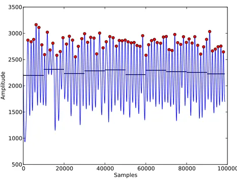
In order to obtain a higher accuracy in detecting signal events, our algorithm updates the threshold every ten seconds. Figure3.1 presents an example of a respiratory signal with the peaks detected using this approach; one can also observe that the horizontal lines are representing the evolution of the threshold (RMS) over time.

(42)

3. SIGNALPROCESSINGALGORITHMS 3.1. Events detection algorithms

0 20000 40000 60000 80000 100000

Samples 500

1000 1500 2000 2500 3000 3500

Amplitude

Figure 3.1: Peaks detections using the RMS of the signal as an adaptive threshold. The horizontal lines represent the evolution of the threshold over time.

meanwavein signals with noise, significant morphological changes or baseline deviations showed better results. Nevertheless, due to its simplicity and low computational cost which is fundamental since our algorithm is also designed to be applied in long duration records, using the signal’s RMS as an adaptive threshold for peaks detections is also an interesting method for accomplishing this step of our algorithm. Once the peaks are detected, a meanwave is also constructed, obtaining one more source of morphological comparison of waves.

3.1.2 Meanwaveapproach

In this sub-section, the implemented events detection algorithm based on the concept of

meanwave is presented. First, an algorithm overview is shown (see sub-section 3.1.2.1). In sub-section 3.1.2.2, the basic concepts used on our algorithm are characterized, pro-viding the necessary contextual information and in sub-section3.1.2.3, all the algorithm improvements are depicted.

3.1.2.1 Algorithm overview

(43)

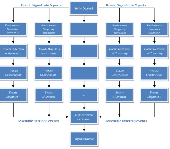
An overview of our events detection algorithm is produced in Figure3.2, where the main building blocks are shown. Due to its applicability to long-term signals, first the signal is divided intoN parts and each one will be processed individually, determining the events of each part. Finally, the results are assembled and the signal events detected.

Raw Signal

Divide Signal intoNparts

Assemble detected events

… Events Detection with overlap Events Detection with overlap Events Detection

with overlap Events Detection with overlap Fundamental Frequency Estimation Fundamental Frequency Estimation Fundamental Frequency Estimation Fundamental Frequency Estimation

Assemble detected events

Waves Construction

Waves

Construction ConstructionWaves

Events Alignment Events Alignment Events Alignment Events Alignment Remove double Detections … … … Signal’s Events

Divide Signal intoNparts

Figure 3.2: Signal Processing Algorithm Steps.

3.1.2.2 autoMeanWavealgorithm

TheautoMeanWavealgorithm has the main goal of detecting events on biosignals and for

that, ameanwaveis automatically computed, capturing the signal’s behaviour. In order to construct themeanwave, the signal must be cyclic and those cycles must be separated, making the fundamental frequency (f0) estimation an essential part of the process [77, 78].

In the autoMeanWave algorithm, the first step consists of estimating the cycles size

(44)

signal first harmonic and, consequently, the signalf0. Hence, the cycles size —winsize—

is estimated and given by:

winsize= fs

f0 ×

1.2 (3.2)

Then, a random part of the original signal (window) with a length ofwinsize(N) is selected and a correlation function is applied to calculate a distance signal showing the difference between each overlapped cycle (signal[i:i+N]) and the window selected at the first place. In Equation3.3it is defined the correlation function used in the autoMean-Wavealgorithm wheredirepresents an element of the distance signal, withiranging from

1 toM₋N, beingM the length of the signal.

di =

PN

j=1|signal[i:i+N]j−windowj|

N (3.3)

Then, the local minima of the distance signal are found and assumed to be the sig-nal events. Fisig-nally, the meanwaveis computed and the signal events are aligned using a reference point which can be chosen among a set of options.

3.1.2.3 Algorithm improvements

Fundamental frequency estimation Although the basic concept of the events detection algorithm was shown in the previous sub-section, some improvements were made and the possibility of applying this algorithm in long-term biosignals was added. In fact, the fundamental frequency estimation is one of the most important parts of our algorithm and an accurate method is extremely necessary.

Beingfeandwinsizeethe estimated fundamental frequency by the algorithm and the

cycles sizes, respectively, two scenarios might arise:

• Iffe ≪ f0, thenwinsizee ≫ winsize. Thus, the length of the distance signal

com-puted by the correlation function will be much smaller and, therefore, the number of local minima will also be smaller. Since the local minima represent the signal events, a great number of events will be dismissed, resulting in a poor estimation of signal’s number of cycles.

• Iffe ≫ f0, thenwinsize_e ≪ winsize. In opposition to the previous scenario, the

length of the distance signal computed by the correlation function will be much greater and, therefore, the number of local minima will also be greater. Thus, a great number of cycles that do not exist will be considered.

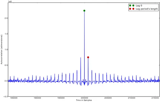
Therefore, instead of determining the first peak of the signal FFT, we used a time-domain method forf0 estimation based on the autocorrelation of time series. Since the

(45)

lag is none, then the waves are in phase and the autocorrelation function reaches a maxi-mum; as the time lag increases to half of the period, the autocorrelation function reaches a minimum since the wave and its time-delayed copy are out of phase. Once the time lag reaches the length of one period, both waves are again in phase and the autocorrelation increases back to a maximum [80].

If we are dealing with an infinite time series,y[n], the mathematical definition of the autocorrelation function is given by the Equation 3.4. Since biosignals are finite time series that could be expressed byx[n], the autocorrelation function is given by Equation 3.5.

Ry(v) =

+∞

X

n=−∞

y[n]y[n+v] (3.4)

Rx(v) = N−1−v

X

n=0

x[n]x[n+v] (3.5)

In order to compute the autocorrelation function, we used the convolution between the signal FFT and the FFT of the signal reversed in time. A representation of the autocorre-lation function and the extracted information from it is presented in Figure3.3.

185000 190000 195000 200000 205000 210000 215000

Tim e in Sam ples 0.5 0.0 0.5 1.0 1.5 2.0 A ut oc or re la ti on ( ad im en si on al ) 1e8 Lag 0

Lag period's length

Figure 3.3: Autocorrelation function of a cyclic signal.

(46)

In order to obtain a more accurate estimation of the fundamental frequency, a quadratic interpolation for estimating the true position of an inter-sample maximum when nearby samples are known was used. Given a functionfand an indexiof that function, the coor-dinatesxeyof the vertex of a parabola that goes through pointiand its two neighbours are given by:

x= 1 2×

f(i₋1)₋f(i+ 1)

f(i₋1)₋2f(i) +f(i+ 1) +i

y=f(i)₋1

4×[f(i−1)−f(i+ 1)](x−i)

Hence, giving as input the autocorrelation function and the peak sample where the lag reaches the length of one period, we obtain the window size using Equation3.2, where f0 =x. However, we widened the window by30%due to the higher accuracy returned

by this method for estimating the fundamental frequency.

It is well known that there are many ways of computing the fundamental frequency since this is a current and active research topic. In fact, an ultimate method forf0

estima-tion is yet to be discovered [80]. However, the autocorrelation approach proved to return more accurate results than the previously presented method.

Events alignment When a more accurate estimation forf0 was implemented, we also

improved the signal events alignment step. In fact, in order to obtain an accurate morpho-logical comparison between waves, an almost perfect alignment of the signal events is required. In [77,78] the alignment is achieved by selecting a notable point from the com-putedmeanwave. For certain types of signals, this led to an inaccurate events alignment and, therefore, an incorrect distance measure between waves and between themeanwave. In order to solve this issue, our algorithm performs two phases of events alignment. First, the events are aligned using a notable point (minimum or maximum value) from the computed meanwave. This notable point is defined as an input of the alignment al-gorithm and if none is given, the maximum value is the default one. Subsequently, our algorithm builds all the waves based on the previously aligned events, where each wave is centred in the correspondent event. The length of a wave,lwave, is given by

comput-ing the differences between two consecutive events and averagcomput-ing those values; thus, the events will be located at the sample lwave

2 of each wave. Finally, our algorithm runs

through all the computed waves and relocates the events to the minimum or maximum value of each wave. Beingeventi(withiranging from 1 tolwave) the final wave-sample

of one event, theshif tithat will be applied to relocate it is given by:

shif ti=eventi−

lwave

2 (3.6)

(47)

to the signal length) the signal-sample of one event, its final position will be given by:

eventj =eventj +shif ti (3.7)

An example of this further events alignment is shown in Figure3.4.

0 100 200 300 400 500 600 700 800 Sam ples 1750 1800 1850 1900 1950 2000 2050 2100 2150 A m pl it ud e

Meanwave alignm ent Wave alignm ent

45000 50000 55000 60000 65000 Sam ples 1800 1900 2000 2100 2200 A m pl it ud e

45000 50000 55000 60000 65000

Sam ples 1800 1900 2000 2100 2200 A m pl it ud e (a) (b) (c)

Figure 3.4: (a) Highlight of event alignment using ameanwaveand a wave reference point; Events alignment in an ECG signal using (b) themeanwave and (c) the wave reference points.

After this final alignment, new waves based on these events are constructed and the distance between each wave and its meanwave is computed, returning accurate wave alignments.

The differences between the two alignment approaches can be observed in Figure3.5. It is important to notice that not only an inaccurate waves alignment leads to incorrect distance measures between the waves and themeanwavebut it also affects its construc-tion.

Long-term biosignals applicability The last improvement made on theautoMeanWave

algorithm is the ability to run over long-term biosignals. In order to accomplish this goal, our algorithm divides the signals intoN parts and each part is processed individually. Hence, beingL the length of the original signal, each part will have a length of Lp =

(48)

0 100 200 300 400 500 600 700 800

Sam ples 1750 1800 1850 1900 1950 2000 2050 2100 2150 A m pl it ud e Waves Meanwave

0 100 200 300 400 500 600 700 800

Sam ples 1750 1800 1850 1900 1950 2000 2050 2100 2150 A m pl it ud e Waves Meanwave (a) (b)

Figure 3.5: Waves andmeanwavealignment and construction using (a)meanwavereference

point and (b) waves reference points.

signal’s fundamental frequency, using larger parts might cause loss of sensitivity to those changes.

To guarantee that no information is lost among transition zones, we introduce af0

-dependent overlap with lengthLo, resulting in a total length for each part ofLpf =Lp+

Lo. The overlap is defined as follows:

1. Select a random part of the signal with length Lp. In our algorithm, the selected

part of the signal is

signalpart=signal

half len₋Lp

2 ;half len+

Lp

2

withhalf lenbeing half of the signal length.

2. Compute the fundamental frequency using the approach described in3.1.2.3.

3. Estimate the cycles size,winsizepart, according to the given information about the

original signal.

4. Define the overlap as

overlap=winsizepart×6

(49)

3. SIGNALPROCESSINGALGORITHMS 3.2. Distance measures

them, the concept of neighbourhood of a number is applied. We define the neighbour-hood (with a radius ofǫ) of a numbernas the set:

Vǫ(n) =]n−ǫ;n+ǫ[ (3.8)

Using Equation3.8and definingǫ= 0.3_×winsizeandn =ei−1 (withiranging from 2

toN), whereei−1is the last detected event of the parti−1, we define the neighbourhood

ofei−1as the set:

V(ei−1) =]ei−1−0.3×winsize;ei−1+ 0.3×winsize[

In order to remove the double detections, if the eventei from part ibelongs to the set

V(ei−1), then all the events that precedeei (including it) are eliminated.

To overcome the obstacle of dealing with large amounts of data, the HDF5 format was used. Hence, the storage of large sized data and its fast access is possible, being these features the main advantages of HDF5 files [81].

Once the events are correctly detected and aligned, distance measures are taken and clustering techniques are applied to obtain signal annotations.

3.2 Distance measures

The previously extracted events allow a duly indication of the signal’s waves. Therefore, distance measures can be taken between waves and between each wave and the signal’s

meanwave.

There are several distance measures that can be applied to one-dimensional arrays and more specifically, to time-series. In order to obtain inputs to our parallel k-means algorithm, we use a set of different distance functions. First of all, the Minkowski-form Distance defined as [61]

Lp(P, Q) =

X

i

|Pi−Qi|p

!1/p

, 1_≤p_{≤ ∞} (3.9)

In this study, we will use theL1,L2andL∞distance functions, which are defined as

L1(P, Q) =

X

i

|Pi−Qi|

L2(P, Q) =

s X

i

(Pi−Qi)2

L∞(P, Q) = max

i |Pi−Qi|

The squared version ofL2,L22, will also be used. Besides, theχ

(50)

3. SIGNALPROCESSINGALGORITHMS 3.2. Distance measures

given by [82]

χ2(P, Q) = 1 2

X

i

(Pi−Qi)2

Pi+Qi (3.10)

will also be utilized to obtain distance measures.

Due to the suitability of our algorithm in long-term biosignals, these distance mea-sures are not represented by a distance matrix. In fact, biosignals can be seen as time-series which have an important feature that allows distance measures without building an extremely high computational cost distance matrix when dealing with long records: the order of relationship between two consecutive samples.

Figure3.6represents a distance matrix for an ECG signal and the highlight of the first

30_×30elements.

0 50 100 150 200

0

50

100

150

200

Distance Matrix for an ECG signal

0 5 10 15 20 25

Highlight for the 30 x 30 first elem ents

0 600 1200 1800 2400 3000 3600 4200 4800 5400 (a) (b)

Figure 3.6: (a) Distance matrix for an ECG signal and (b) the highlight of the first30_×30

elements of the distance matrix.

Observing the 30_×30 distance matrix, it is clear that the observations number 11, 12, 13 and 14 are significantly different from the other ones, resulting in two transition zones: the transition from the10thobservation to the11thand from the14thobservation to the15th_{. Since we are dealing with time-series, the concept of transition zone is valid}

and therefore, instead of searching for the resemblance between each observation and the other ones to build a distance matrix, it is only necessary to find the transition zones.

(51)

3. SIGNALPROCESSINGALGORITHMS 3.3. Parallelk-means algorithm

by:

ai=f(wi, wi+1),i= 1, . . . , n−1 (3.11)

beingf the distance function andnthe number of waves, representing also the number of events detected by the previous step of our algorithm.

In the particular case wherewi =mw, wheremwdenotes the signal’smeanwave, then

each element of the distance array will be:

ai =f(mw, wi),i= 1, . . . , n (3.12)

Although the distance matrix carries richer information about waves resemblance than the distance array, its high computational cost makes it impracticable in long records.

Using this set of distance functions, a comparison between the efficiency of each one as an input for our clustering algorithm will be made, allowing to state which is the most adequate distance function for morphological analysis in biosignals.

3.3 Parallel

k

-means algorithm

As the final step of our algorithm, a parallelk-means was implemented, being able to per-form unsupervised learning on long-term biosignals. The main concept of thek-means

algorithm was kept [49,50], which is a partitioning method for clustering where data is divided intokpartitions [38]. The optimal partition of the data is obtained by minimizing the sum-of-squared error criterion with an interactive optimization procedure. Cluster-ing algorithms can perform hard-clusterCluster-ing when each cluster can only be assigned to one partition; otherwise, they perform fuzzy-clustering. Our algorithm was designed to perform hard-clustering since it was based in thek-means hard clustering algorithm.

As an additional modification to the originalk-means, we also introduceniterations to the algorithm in order to minimize one of the biggest drawbacks related to the initial partition. In fact, different initial partitions usually converge to different cluster groups [5,6].

As Figure3.7suggests, the parallelk-means algorithm receives as input a set of ob-servations. These observations come from the distance measures previously presented. In order to run this parallel version of thek-means algorithm over large sized data, the observations (with the initial length ofM) are divided intoN parts. Due to the fixed size of each part, the last part might be smaller than the remaining ones.

After dividing the observations into parts, our algorithm performs thek-means

clus-tering algorithm in each part individually. For each part a different set of k centroids will be obtained. Theithpart, for example, will have the centroids[a_i_,b_i_{, . . . ,}k_i_], with_i

ranging from 1 toN. It is important to notice that if each observation isn-dimensional, each centroid will also ben-dimensional.