Ricardo Daniel Domingos Chorão

(1)

Ricardo Daniel Domingos Chorão

Licenciatura em Ciências de Engenharia Biomédica

Parallel Programming in Biomedical Signal

Processing

Dissertação para obtenção do Grau de Mestre em Engenharia Biomédica

Orientador: Prof. Doutor Hugo Filipe Silveira Gamboa

Júri:

Presidente: Prof. Doutor Mário António Basto Forjaz Secca

Arguentes: Prof. Doutor José Luís Constantino Ferreira

Vogais: Prof. Doutor Hugo Filipe Silveira Gamboa Prof. Doutor José Luís Constantino Ferreira

(2)

(3)

iii

Parallel Programming in Biomedical Signal Processing

Copyright c Ricardo Daniel Domingos Chorão, Faculdade de Ciências e Tecnologia, Universidade Nova de Lisboa

(4)

(5)

(6)

(7)

Acknowledgements

In the end of one of the most prolific periods of my life, I would like to thank the people that made this rewarding learning experience possible.

First of all I would like to thank Professor Hugo Gamboa for welcoming at PLUX -Wireless Biosignals, S.A. and for agreeing to work with me during the last semester of a 5 year academic route. Your guidance and the discussions we had proved invaluable and have given me a new perspective when I needed it.

I am also grateful to all the staff at PLUX for the kind and humorous moments we shared in the last months and for making me feel welcome and part of a great team.

I want to thank Joana Sousa for her support and for pushing me further, helping me to achieve more.

I am also thankful to Doctor Mamede de Carvalho, for helping me acknowledge the potential of the developed work.

My sincere appreciation to Neuza Nunes for enlightening me when I most needed and for always helping me to learn with my mistakes.

A special thanks to my friends Nuno Costa, Rodolfo Abreu, Angela Pimentel and Diliana Santos. Your support helped keeping me motivated and it was a pleasure to have you around.

I am also grateful to my good friend Sara Costa, Sérgio Pereira, João Rafael and Ana Patrícia for their support during these last years of my life and for all the laughs we shared.

(8)

(9)

Abstract

Patients with neuromuscular and cardiorespiratory diseases need to be monitored continuously. This constant monitoring gives rise to huge amounts of multivariate data which need to be processed as soon as possible, so that their most relevant features can be extracted.

The field of parallel processing, an area from the computational sciences, comes nat-urally as a way to provide an answer to this problem. For the parallel processing to suc-ceed it is necessary to adapt the pre-existing signal processing algorithms to the modern architectures of computer systems with several processing units.

In this work parallel processing techniques are applied to biosignals, connecting the area of computer science to the biomedical domain. Several considerations are made on how to design parallel algorithms for signal processing, following the data paral-lel paradigm. The emphasis is given to algorithm design, rather than the computing systems that execute these algorithms. Nonetheless, shared memory systems and dis-tributed memory systems are mentioned in the present work.

Two signal processing tools integrating some of the parallel programming concepts mentioned throughout this work were developed. These tools allow a fast and efficient analysis of long-term biosignals. The two kinds of analysis are focused on heart rate variability and breath frequency, and aim to the processing of electrocardiograms and respiratory signals, respectively.

The proposed tools make use of the several processing units that most of the actual computers include in their architecture, giving the clinician a fast tool without him hav-ing to set up a system specifically meant to run parallel programs.

(10)

(11)

Resumo

Os pacientes com doenças neuromusculares e cardiorespiratórias precisam de ser mo-nitorizados continuamente. Esta monitorização origina grandes quantidades de informa-ção multivariada que precisa de ser processada em tempo útil, de modo a que possa ser feita a extracção das caracteristícas mais importantes.

O processamento paralelo, inserido na área das ciências da computação, surge natu-ralmente como uma forma de dar resposta a este problema. Para que o processamento paralelo tenha sucesso é necessário que os algoritmos existentes de processamento de si-nal sejam adaptados às arquitecturas modernas de sistemas computacionais com vários processadores.

Neste trabalho são aplicadas técnicas de processamento paralelo de biosinais, conju-gando o domínio computacional e o domínio biomédico. São feitas várias considerações acerca de como desenhar algoritmos paralelos para processamento de sinal, seguindo so-bretudo o paradigma de programação "data parallel". A ênfase é dada ao desenho de algoritmos e não aos sistemas computacionais que os executam, apesar de serem aborda-dos os sistemas de memória partilhada e de memória distribuída.

Foram desenvolvidas duas ferramentas de processamento de sinal que integram al-guns dos conceitos de paralelismo mencionados ao longo do trabalho. Estas ferramentas permitem uma análise rápida e eficiente de biosinais de longa-duração. Os dois tipos de análise feita incidem sobre a variabilidade da frequência cardíaca e sobre a frequência respiratória, partindo de sinais de electrocardiograma e de respiração, respectivamente.

As ferramentas fazem uso das várias unidades de processamento que a generalidade dos computadores actuais apresenta, proporcionando ao clínico uma ferramenta rápida, sem que este tenha a necessidade de montar um sistema dedicado para a execução de programas em paralelo.

(12)

(13)

List of Figures

2.1 The respiratory signal is generated by the force exerted by the chest on a piezoelectric material. The deformation of the material is proportional to the expansion of the rib cage and is translated into the amplitude of the signal.. . . 6

2.2 A typical ECG, with highlighted features. . . 7

2.3 Two RR measurements between three consecutive heart beats. . . 8

2.4 From [1]. The data acquisition system converts the analog signal into a digital signal that can be stored. Signal processing techniques may then be applied to reduce the noise (signal enhancement). . . 10

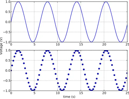
2.5 The analog signal and the corresponding digital signal. . . 11

2.6 A pre-processing technique. Here, the noise is removed from the signal by application of a low-pass filter in the frequency domain. . . 11

2.7 These screenshots show the CPU usage over time in a system with 2 cores. 13

2.8 An example of a distributed computation. The problem consists of com-puting the sum of a large set of numbers. The data is partitioned so that each computing node sums each partition. Finally, the master computer only has to sum the results. . . 15

2.9 A pipelined computation. There are precedence constraints between the different pipelined processes. . . 17

2.10 Schematic of aMapReducecomputation . . . 17

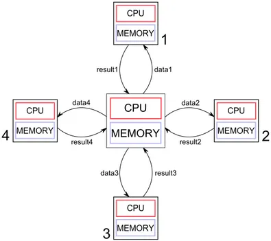
3.1 Master-slave distributed parallel computing architecture best suited to run the developedMapReducederived algorithms. . . 20

3.2 Schematic of the whole computation. In this situation the division of the long-term record gives rise to 4 data-structures, which are processed in 4 computing nodes, prior to the application of thereducefunction by the master computer. . . 24

(16)

xvi LIST OF FIGURES

4.2 Programming architecture of the signal processing tool. . . 31

4.3 Multilevel visualization of a 7 hour long ECG . . . 31

4.4 The user only wishes to analyse the portion of the signal between the dashed lines (0.85 s to 4.43 s). Of the 6 total peaks, only 4 of them are retrieved and 3 RR intervals are computed (out of the total 5). . . 33

4.5 1. Report Generation; 2. Programming mode analysis; 3. On-screen analysis. 34

4.6 The most important parameters and visual representations provided by the on-screen HRV analysis. . . 35

4.7 Four pages of a HRV analysis report from a night record. . . 37

4.8 Detection of respiratory cycles using an adaptive threshold, which changes every 5 seconds . . . 39

4.9 On-screen analysis of a portion of a respiratory signal.. . . 40

5.1 Execution times of the ECG peak detection algorithm in a 8 core remote virtual machine. . . 46

5.2 ECG peak detection algorithm mean execution time and the expected exe-cution time. . . 47

5.3 Execution times of the respiratory cycles detection algorithm in a 8 core remote virtual machine. . . 48

(17)

List of Tables

5.1 AWS virtual machine features . . . 44

5.2 Performance analysis of the ECG peaks detection algorithm. . . 47

(18)

(19)

Acronyms

AAL Ambient Assisted Living

ALS Amyotrophic Lateral Sclerosis

ANS Autonomic Nervous System

AWS Amazon Web Services

BVP Blood volume pressure

CPU Central Processing Unit

ECG Electrocardiogram

GUI Graphical User Interface

GPU Graphical Processing Unit

HDF5 Hierarchical Data Format 5

HRV Heart Rate Variability

PSD Power Spectral Density

RAM Random Access Memory

RMS Root Mean Square

SFTP Secure Shell File Transfer Protocol

(20)

(21)

1

Introduction

1.1 Motivation

The ever increasing development of clinical systems for continuous monitoring of pa-tients’ biosignals has become widely available, not only in clinical facilities but also at home in an ambient assisted living (AAL) environment.

The continuous monitoring of the patients vital signals gives rise to huge amounts of data which need to be processed as soon as possible. The collected information is most of the times multivariate data, composed by many types of biosignals, all of them acquired simultaneously. Examples of such biosignals are the electrocardiogram, respiration, elec-troencephalogram or electromyogram [2].

The detection of changes in the patients state must be fast and reliable in order to act in a preventive manner and avoid complications for the subject. This detection is achieved through the extraction of relevant features from the collected data.

Real-time analysis is a common practice nowadays. The most illustrative example is the real-time QRS detector and its well known beep noises, each one representing one heartbeat. There are other types of analysis that can only be done after the data acquisi-tion process is finished. This long-term analysis may be very significant since it allows the assessment of the evolution of the patients’ vital signals over a long period of time. Moreover, the analysis of long-term biosignals allows the detection of low-frequency phe-nomena, which can not be analysed otherwise.

(22)

1. INTRODUCTION 1.2. State of the art

algorithm).

One of our goals was also to make the developed parallel processing algorithms ac-cessible to the clinician and the researcher, so that in order to apply them to long-term records one does not need to have programming skills.

We also introduce some guidelines to design parallel algorithms following the data parallel model, in a very similar way to theMapReduceprogramming model [3].

This work was developed in cooperation with PLUX, Wireless Biosignals, S.A. [4], which kindly provided the long-term biosignals that allowed to test the performance of the developed algorithms and signal processing tools. The biosignals were acquired by amyotrophic lateral sclerosis patients.

1.2 State of the art

The application of parallel programming techniques to biomedical signal processing is not entirely new. In the field of biomedical image processing (which is typically compu-tationally intensive), parallel programming is used frequently with graphical processing units (GPUs) instead of the commonest central processing units (CPUs) to process the data [5,6].

In the field of bioelectric signals, parallel processing techniques have been used with several purposes, namely filtering [7], independent component analysis [8] (a common electroencephalogram analysis technique) and ECG QRS detection [9].

In this work some of these techniques are used in the design of parallel algorithms. These algorithms are to be part of heart rate variability and respiratory analysis tools.

There are several heart rate variability analysis tools, such as "Biopac HRV Algorithm" [10], "HRVAS: HRV Analysis Software" (using MatLab) [11] and "HRV Toolkit" (Phys-ionet). They all provide frequency and time domain analysis of ECG records. However they lack interactivity and do not allow one to deal directly with long duration ECGs, both in the visualization and in the processing parts. Moreover, the available tools do not work from the raw ECG. It is assumed that the QRS complexes were previously de-tected elsewhere. This dependency of another tool to process the ECG directly is notuser friendly. HRV analysis tools such as the HRVAS include parallel processing in its HRV analysis. However the program crashes when attempting to analyse long-term records. Another problem with some of these tools is that they are based on proprietary software, and therefore are notopen source, which was our intent.

(23)

1. INTRODUCTION 1.3. Objectives

Regarding the analysis of respiratory records, to our knowledge that kind of analysis is not incorporated in any signal processing tool. There are many examples in the litera-ture of the analysis of respiration, extracted from ECG records and not from respiratory records themselves [12,13,14]. The respiratory analysis from respiratory records rather than from ECG records is more accurate. To design and develop a tool that performs such an analysis (and especially over long-term records), would represent an innovation in the biosignal processing area.

1.3 Objectives

The main goal of this work is the application of parallel programming techniques in the field of biomedical signals processing. The application of such techniques arises from the need to process long-term multivariate data, obtained from continuously monitoring patients. For that, several parallel algorithms, following the data parallel programming model and a model similar to the MapReduce[15] programming model were designed, the most important being a ECG QRS detector and a respiratory cycles detector.

Another objective of this work was to make the developed parallel algorithms acces-sible to the clinician and the researcher, even if they do not have a background in pro-gramming. To address this particular goal, the algorithms were integrated in a biosignals processing tool, in two modules:

1. a heart rate variability (HRV) analysis tool;

2. a respiratory analysis tool.

The proposed tools are highly portable and user friendly and allow an efficient pro-cessing of long duration biosignals.

The developed tools are particularly suited for the analysis of long-term records, since they were integrated in a previously existing tool which aimed at the visualization of long-term biosignals [16]. This way, the user is able to thoroughly inspect the biosignals and the processing results simultaneously, in a synchronized way, making it much easier and faster to unravel fundamental analysis features.

(24)

(25)

2

Concepts

In this chapter, some concepts with relevance to the comprehension of this work are pre-sented. They range from biosignals to parallel computing and parallel programming models, and its application in the analysis of biosignals.

2.1 Biosignals

Biosignal is a term that represents all kinds of signals that can be recorded from living beings. They are typically recorded as univariate or multivariate time series and contain information related to the physiological phenomena that originated them. This infor-mation can be extracted by signal processing techniques and may then be an important input for clinical research or medical diagnosis.

As it will be presented in the next section, there are several types of biosignals, its nature ranging from electrical to mechanical. Special emphasis will be given to the elec-trocardiogram (ECG) and to the respiratory signals since an important part of this work is focused on their analysis.

2.1.1 Biosignals types

(26)

2. CONCEPTS 2.1. Biosignals

processing has made it possible to understand that, as the organ systems in our body are connected and do not behave independently, so it is with biosignals. This connection allows us to draw conclusions from biosignal analysis and feature extraction that would not seem relateda priorito the nature of the biosignals.

Biosignals may have several physiological origins, according to which they are clas-sified. In this work, the biosignal types used were [1,2]:

• Bioelectric signals: these signals are generated by nerve or muscle cells. In this sit-uation anaction potentialis measured with surface or intramuscular electrodes. The electrocardiogram, electromyogram and the electroencephalogram are examples of such signals;

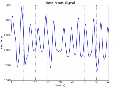
• Biomechanical signals: these signals are produced by measurable mechanical func-tions of biological systems, such as force, tension, flow or pressure. Examples of such signals are the BVP (blood volume pressure), accelerometry (which mea-sures acceleration) and the respiratory signal, which is acquired with a piezoelec-tric transducer, typically placed in the chest. An example of a respiratory signal is depicted in figure2.1.

Other types of biosignals are biomagnetic signals, biochemical signals, bioacoustic signals and biooptic signals.

0 5 10 15 20 25 30 35 40

tim e (s) 1000

1500 2000 2500 3000 3500

am

pl

it

ud

e

Respiratory Signal

Figure 2.1: The respiratory signal is generated by the force exerted by the chest on a piezoelectric material. The deformation of the material is proportional to the expansion of the rib cage and is translated into the amplitude of the signal.

Electrocardiogram

(27)

P

Q R

S

T

ST Segment PR

Segment

PR Interval

QT Interval QRS

Complex

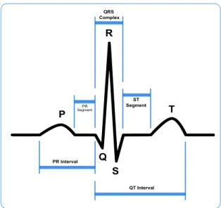
Figure 2.2: A typical ECG, with highlighted features.

Each feature highlighted in fig.2.2corresponds to a different event in the cardiac cycle. The first deflection, the P wave corresponds to current flows during atrial depolariza-tion. It has a duration of 80-100 ms. The PR interval, with a typical duration of 120-200 ms, represents the onset between atrial and ventricular depolarization. A PR interval greater than 200 ms indicates an AV conduction block.

The QRS complex, the most prominent feature of the ECG, is the result of ventricular depolarization. Its normal duration is 60-100 ms. If the QRS complex duration is greater than 100 ms, there may be a block in the impulse path, which results in the impulses being conducted over slower pathways within the heart.

The T wave is the result of ventricular repolarization. Atrial repolarization does not usually show on an ECG record because it occurs simultaneously to the QRS complex [17].

The shapes and sizes of the P wave, QRS complex and T waves vary with the elec-trodes locations. Therefore, it is a typical clinical practice to use many combinations of recording locations on the limbs and chest (ECG leads) [18,17].

When a muscle contracts, it generates an action potential. After that, there is a long

absolute refractory period, which, for the cardiac muscle, lasts approximately 250 ms. Dur-ing this period the cardiac muscle can not be re-excited, which results in an inability for heart contraction [18]. Therefore, a theoretical heart rate limit of about 4 beats per second, or 240 beats per minute can be considered.

Respiration

(28)

consists of oscillations, more or less periodical. The measurement units are amplitude, since what matters is the displacement of every respiratory cycle, relative to each other. In chapter4the amplitudes are normalized so that the observable amplitude values are not dependent on the gain factor of the acquiring device. The spacing between every breath (also referred in this work as a respiratory cycle) allows the calculation of the breath frequency. In the respiration tool described in chapter4the maximum breath frequency is considered to be 40-60 cycles/minute [19]. This limit is important from an algorithmic standpoint because it allows the rejection of respiratory cycles which are detected less than 1s apart (detection errors).

2.1.2 Heart rate variability

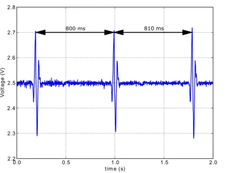
Heart rate variability (HRV) is a method of physiologic assessment which uses the oscilla-tions between consecutive heart beats to evaluate the modulation of the heart rate by the autonomic nervous system (ANS) [20]. HRV is also referred to as RR variability because of the way these oscillations are typically extracted from an ECG record - by measuring the RR intervals, as depicted in fig.2.3.

0.0 0.5 1.0 1.5 2.0

tim e (s) 2.2

2.3 2.4 2.5 2.6 2.7 2.8

V

ol

ta

ge

(

V

)

800 ms 810 ms

Figure 2.3: Two RR measurements between three consecutive heart beats.

There are many HRV analysis techniques, the most important being frequency do-main analysis and time dodo-main analysis [21].

(29)

Frequency domain analysis of HRV is based on power spectral density (PSD) analysis of RR intervals and provides basic information about how power distributes as a function of frequency. The power related to different bands relates to different branches of the ANS, which makes the power distribution a very important tool to identify ANS related problems.

HRV analysis has many clinical applications, posing as an indicator of certain dis-eases. Several studies state the reduced HRV in patients with amyotrophic lateral scle-rosis (ALS) [22,23]. In normal subjects, large changes in successive RR intervals (> 50 ms) occur frequently, but irregularly. In patients with diabetes, reduced HRV may help detecting early cardiac parasympathetic damage [24].

2.1.3 Respiratory analysis

The analysis of respiratory signals has applications in several fields, namely:

• In diagnosing sleep disorders, such as sleep apnea, characterized by pauses in breathing or abnormally low breathing during sleep [25];

• Assessment of mental load and stress and detection of emotional changes [26];

• Respiratory monitoring in athletes to determine ventilation levels and study the relation with their performance [27].

2.1.4 Biosignals acquisition

In biosignals acquisition, the sensor is the part of the instrument that is sensible to varia-tions in the physical parameter to be measured. The sensor must be specific to the nature of the biosignal to be measured. It provides an interface between the biological medium and electrical recording instruments, by converting the physical measurand into an elec-tric output.

High-precision, low-noise equipment is often needed, because the signal (which is normally small in amplitude) typically contains unwanted interferences. Such interfer-ences may be the 50 Hz noise from the electronic equipment, caused by the lighting sys-tem or intrinsic interferences like the contamination of an ECG record by the electric activity of adjacent muscles.

The typical steps followed throughout data acquisition are depicted in figure2.4

Because the signals will most likely be used for medical diagnostic purposes, it fol-lows that the information contained in them must not be affected or distorted by ampli-fication, analog filtering or analog-to-digital conversion.

(30)

Figure 2.4: From [1]. The data acquisition system converts the analog signal into a digital signal that can be stored. Signal processing techniques may then be applied to reduce the noise (signal enhancement).

original signal, it is only an approximation. It is generated by repeatedly sampling the amplitude of the analog signal at fixed time intervals. The inverse of that time interval is called the sampling frequency of the digital signal. Figure2.5illustrates this sampling process.

Besides the sampling frequency, there is another process which affects the degree of similarity between the original analog signal and the digital one called quantization. As mentioned, a numerical value is assigned to a particular amplitude in the A/D converter. Quantization reduces the infinite number of amplitudes (a continuous interval) into a limited set of values. The A/D converter resolution determines the number of bits of the signal values. The typical number of bits of the discrete samples is 8, 12 or 16, for most A/D converters. An insufficient number of bits can lead to information loss during the conversion process, which in turn may lead to errors in the interpretation of the data.

The sampling frequency, if too low, can lead to the same problems as low A/D con-verter resolution. If too high, however, it may give rise to the generation of huge data col-lections, especially when we are dealing with long duration records, for example whole nights. To process that data in a reasonable amount of time, we may need parallel pro-gramming techniques.

2.1.5 Biosignals processing

Biomedical signals processing is an intermediate step between acquiring the signal and drawing conclusions from the data.

Most of the times, the relevant information to be extracted from a record is concealed, not directly seen through raw data observation. The aim of digital signal processing is revealing those "hidden" signal features, with relevance for direct analysis [2].

(31)

2. CONCEPTS 2.2. The Hierarchical Data Format 5

0 5 10 15 20 25

1.0 0.5 0.0 0.5 1.0

0 5 10 15 20 25

time (s) 1.0

0.5 0.0 0.5 1.0

Voltage (V)

Figure 2.5: The analog signal and the corresponding digital signal.

a pre-processing phase, in order to make the data suitable for further analysis. A typical pre-processing technique, noise removal, is illustrated in figure2.6.

Signal+noise FFT Low-pass filter Inverse FFT Signal

Figure 2.6: A pre-processing technique. Here, the noise is removed from the signal by application of a low-pass filter in the frequency domain.

After the pre-processing phase, the signal is ready for features extraction and inter-pretation.

The algorithms applied make possible not only an enhanced signal visualization, but also the signals statistical analysis and the extraction of certain parameters, specific of the nature of the biosignals. One example of a such algorithm is an algorithm that detects the R times in an ECG record.

2.2 The Hierarchical Data Format 5

(32)

2. CONCEPTS 2.3. Central processing unit

the data, as well as writing data to the files at very high speeds [28].

By continuously monitoring patients, remotely or in a medically controlled environ-ment, huge amounts of data are generated. In healthcare, a fast response to evidence of a medical condition or disease is of paramount importance and can save lives. Hence the pressing need for fast data processing and analysis. Because of the above, *.hdf5 (or *.h5) files are suitable for storage of long duration biosignals and subsequent analysis.

H5 files have a hierarchical structure composed by two types of objects:

• Groups - a group is a container structure, similar to a folder. A group may contain an arbitrary number of other groups and datasets;

• Datasets - a dataset is the structure that contains the data. The data in a dataset must be of homogeneous type, but in the same file several datasets may hold data of different types.

This file format also supports the introduction of metadata called attributes. Each group can have its own attributes and the file, as a whole structure can have attributes associated too. When the files contain medical information - such as recorded biosignals -, the attributes are very useful to store key information about the subject, the type of the record or the data. Such attributes may be the acquisition date and time length of the record, the sampling frequency or the patient’s name.

To manage files in this format, there is a Python[29] library called h5py [30]. This library allows file writing and data manipulation in a very convenient way, in a manner which is similar to another scientificPythonlibrary, thenumpy[31].

2.3 Central processing unit

A resource is any component with limited availability within a computer system . This section provides a description of the most important system resource to account for when dealing with parallel programming - the CPU. Examples of other important resources are the, random access memory (RAM) hard disk space or a network throughput.

The CPU is the most important system resource concerning parallel programming. The whole point of dividing a problem into several tasks and run them concurrently is to be able to use more computational power at the same time.

(33)

2. CONCEPTS 2.3. Central processing unit

scheduler) is the part of the kernel that determines when and for how long a process is allowed to run [32].

A parallel job scheduler allocates nodes for parallel jobs and coordinates the order in which jobs are run. While several jobs are executed simultaneously, others are enqueued and wait for nodes to become available. Two very important goals of a scheduler are the optimization of the number of jobs completed per unit of time and keeping the utilization of computer resources high [33].

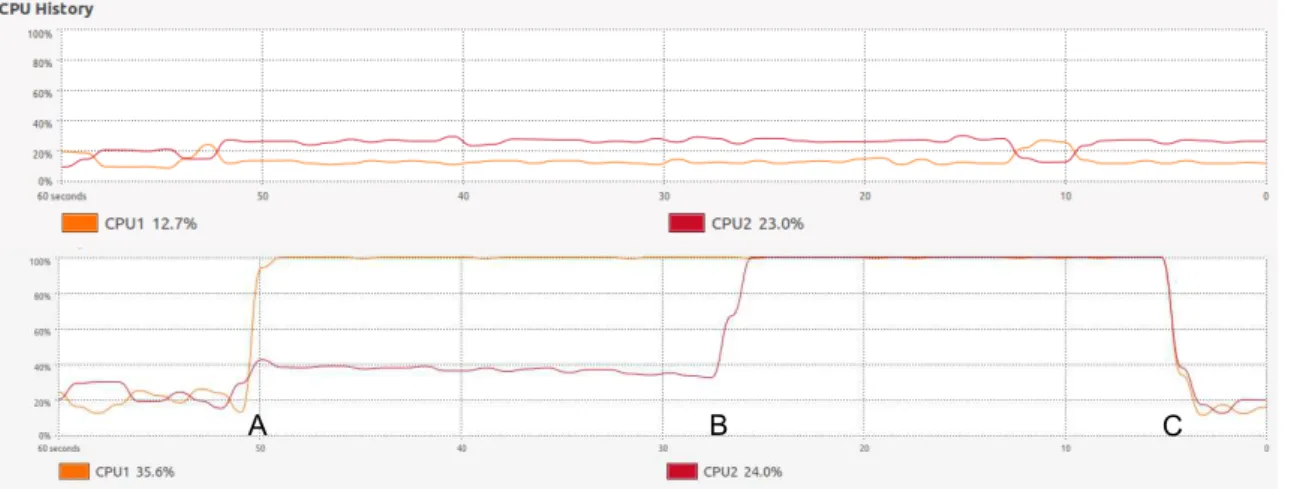
In computers with multiple processors, true parallelism can be achieved because dif-ferent programs can be run at exactly the same instant in difdif-ferent processors. In each processor, the scheduling of the different processes takes place.

When a sequential program is run in a system with multiple processors, the program runs in a single processor. For the program to be executed by multiple processors, some specification must be given by the user, identifying the parts that can be run in parallel.

Figure 2.7 illustrates this concept. It consists of two screenshots from a dual core Ubuntu machine, during the execution of a program. Initially the system is idle and there is low CPU usage in both cores. There are small oscillations in the CPU usage related to background processes.

A B C

Figure 2.7: These screenshots show the CPU usage over time in a system with 2 cores.

(34)

2. CONCEPTS 2.4. Parallel programming

2.4 Parallel programming

2.4.1 Overview

Nowadays, computers with multiple processors are widely available. The total compu-tational power of such computers is inexpensive, if we were to compare it with a single central processing unit (CPU) with the equivalent computational power.

According to Moore’s law [34], the number of transistors that can be placed on a chip doubles every two years. This trend drove the computing industry for 30 years, leading to increased computer performance, while decreasing the size of chips and increasing the number of transistors they contained . However, transistors can’t shrink forever, namely because of heat generation. In 2004, a point was reached where performance increases slowed to about 20 % a year. In response, manufacturers are building chips with more cores instead of one increasingly powerful core [35].

A single core processor runs multiple programs "simultaneously" by assigning time slices to each program, which may cause conflicts, errors and slowdowns . Multicore pro-cessors increase overall performance by being able to handle more work in parallel. The different cores can share on-chip resources, which reduces the cost of communications, as opposed to systems with multiple chips [36].

To take advantage of this new architecture, a new way of thinking must be employed, and so has the way how software and algorithms are designed. This way of designing algorithms is called parallel programming.

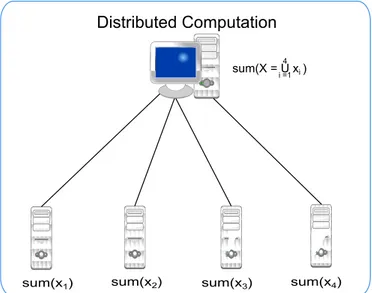
In parallel programming, a single problem is divided into several tasks that can be solved concurrently by different processing units. This approach allows faster problem solving by increasing the overall computational power and makes it possible to tackle problems that require huge amounts of memory and time to be solved and that could not be solved otherwise. The total CPU time required to solve a problem is the same or even higher than the CPU time it would take for the problem to be solved using a single processor. However, the human time it takes for the problem to be solved is much lower. A schematic of a distributed computation, taking place in different computing units can be seen in fig.2.8.

A number of complex problems in science and engineering are called "grand chal-lenges" and fall into several categories, such as [37]:

• Quantum chemistry, statistical mechanics and relativistic physics

• Weather forecast

• Medicine, and modelling of human bones and organs

• Biology, pharmacology, genome sequencing, genetic engineering

(35)

Distributed Computation

Figure 2.8: An example of a distributed computation. The problem consists of computing the sum of a large set of numbers. The data is partitioned so that each computing node sums each partition. Finally, the master computer only has to sum the results.

The computing platform may be a multicore computer or several independent com-puters connected in some way, i.e., a computer cluster.

The main idea is thatncomputers can provide up tontimes the computational speed of a single computer, with the expectation that the problem can be completed in1/nth_of the time [38]. This is of course an ideal situation, which does not occur in practice, except for some embarrassingly parallel applications - applications that are parallel in nature -, such as Monte Carlo simulations.

Theoretically, the maximum speedup of a parallel program is limited by the fraction of the program that can not be divided into concurrent tasks - serial fraction of the prob-lem. The maximum speedup of a parallel program is given by Amdahl’s law [38,37] in equation2.1.

S(n) = ts

f ts+ (1−f)ts/n =

n

1 + (n−1)f (2.1)

WhereS is the speedup,nis the number of processors,f is the fraction of the com-putation that is computed sequentially andtsis the time the serial execution would take. If the sequential fraction of the program is 0, an ideal situation, the speedup isn, that is, the execution time is reduced by1/n. Withf different than 0, as occurs in practice, the maximum speedup is given by:

lim

n→∞S(n) =

1

f (2.2)

(36)

in parallel).

The efficiency and speedup factor, two performance related concepts are only defined in chapter5where it is most appropriate due to the nature of the chapter.

The holy grail of parallel computing is the automatic parallelization of a sequential problem by a compiler. The compiler would on its own identify the existing parallelism within the program and assure its concurrent execution. Such a compiler does not exist yet, and automatic parallelization only had a limited success so far [39]. There are some programming languages such as Chapel [40], Parallel Haskell [41] and SISAL [42], but in all of them the user must identify with some language construct the parts of the program that can be run in parallel.

2.4.2 Programming models

Regarding problem decomposition, there are two main programming models: data par-allelism and control parpar-allelism. A brief introduction to data parpar-allelism and to pipeline parallelism, a special case of control parallelism, is given below:

2.4.2.1 Data parallelism

In data parallelism, multiple processing units apply the same operation concurrently to different elements of a data set. This is the case in the example of figure2.8. The main feature of data parallel algorithms is their scalability ,i.e., a k-fold increase in the number of processing units leads to a k-fold increase in the throughput (number of results pro-cessed per unit of time) of the system, provided there is no overhead associated with the increase in parallelism [37]. In biosignals processing the data parallel approach is quite attractive, especially if we are dealing with huge datasets, which cannot all be processed at once. In the following section, a type of data parallel algorithms, called Map Reduce algorithms is presented.

2.4.2.2 Pipelined parallelism

(37)

P0 P1 P2 P3

Figure 2.9: A pipelined computation. There are precedence constraints between the dif-ferent pipelined processes.

2.4.3 MapReducealgorithms

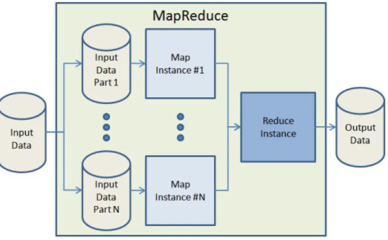
MapReduceis a style of computing - programming model and associated implementation -, originally implemented byGoogle. The programming model was presented by the first time by Dean and Ghemawat in 2004 [15]. A schematic of the computation can be seen in fig.2.10.

Figure 2.10: Schematic of aMapReducecomputation

All the user needs to do is write two functions calledMapandReduce. TheMap func-tion processes a key/value pair and generates a set of intermediate key/value pairs; the

Reducefunction merges all the intermediate values associated to the same intermediate key.

Programs written in this way are easily parallelized and executed on a large cluster of commodity machines. This implementation is therefore highly scalable.

The system manages the parallel execution in a way that is tolerant to hardware fail-ures, while coordinating the task distribution between the compute nodes. MapReduce

can be viewed as a library which is imported in the beginning of the problem and han-dles all the details concerning parallelization, hiding them from the programmer.

A typicalMapReduceexample is the "word count" problem. In this problem the return value is the number of occurrences for each word in a collection of documents.

The computation executes as follows [3]:

(38)

may read a whole document and break it into its sequence of wordsw1, w2, . . . , w_n.

The output of the Map task is a sequence of key/value pairs:

(w1,1),(w2,1), . . . ,(w_n,1)

2. The key/value pairs resulting from each Map task (each Map task could be related to a different file) are sorted by key. The sorted key/value pairs are then aggregated. The obtained sequence is of the form:

(w1,[1,1,1]),(w2,[1,1]), . . . ,(wn,[1,1,1,1])

This step is sometimes called "Grouping and Aggregation".

3. Finally, the Reduce task takes input pairs consisting of a key and its list of associated values, and combines those values in a way that was previously specified. The output of the Reduce task is a sequence of key/value pairs consisting of the input key paired with a value, constructed from the list of values received along with that key. In the "word count" example the Reduce task simply has to sum the values in the lists associated to each key. The final result would then be:

(w1,3),(w2,2), . . . ,(w_n,4)

A programming model very similar to MapReduce is described in chapter 3, along with examples of parallel algorithms that follow this model. Because the programming model is not exactly the same asMapReduce, the algorithms are called in this work " MapRe-ducederived algorithms" and are applied in the area of biomedical signal processing. The main similarity withMapReduceis the need to define two functions to tackle a problem (a map and a reduce function). The main differences are:

• The map function does not necessarily process key/value pairs - the input data structures may be more complex, and always include a part of the signal to process;

(39)

3

MapReduce Derived Algorithms

In this work, a set of algorithms following theMapReduceprogramming model were de-veloped. They were calledMapReducederived algorithms because of the existing similar-ities between the thought process which originated them and theMapReduce program-ming model itself. In this chapter the underlying programprogram-ming strategy is described and some examples are presented.

3.1 Computing architecture

The developed algorithms are the parallel versions of the algorithms of an HRV analysis tool, adapted to the analysis of long-term records. The adopted programming model offers high scalability, since the algorithms are meant to be run in a distributed system. The idea of analysing clinical data using a programming model similar to MapReduce is recent and not widespread [43,44]. The architecture that better suits the correct operation of these algorithms is illustrated in figure3.1.

The master-slave architecture (also called master-worker model) is characterized by the existence of a master computer which controls the execution of the program [45]. In this model, the master processor executes the main function of the program and dis-tributes work from the central node to worker processors [33], hence being responsible for worker coordination and load-balancing. According to this model, there is no com-munication between the workers, whatsoever.

(40)

3. MAPREDUCEDERIVEDALGORITHMS 3.1. Computing architecture CPU MEMORY CPU MEMORY CPU MEMORY CPU MEMORY CPU MEMORY

1

2

3

4

data3 result3 result1 data1 data2 result2 data4 result4

Figure 3.1: Master-slave distributed parallel computing architecture best suited to run the developedMapReducederived algorithms.

more flexibility.

The data parallel model is applied to achieve higher scalability, by partitioning the data. The implementation of this model is very common in scientific computing [46]. By partitioning the data further and further the number of computer nodes (and the overall computing power) is increased, and the original problem may be solved faster. This partitioning process can not be done indefinitely, i.e. there are a few factors that might limit the extent to which the data can be divided. They are:

• The nature of the algorithm: the algorithm may require a minimum amount of signal samples to perform well, and therefore dividing the signals past that limit is counterproductive;

• The task(s) assigned to each computing node should contain enough computations so that the task execution time is large compared to the scheduling and mapping time required to bring the task to execution [45]. The size of a task is described by its granularity. In coarse granularity, each task takes a substantial time to execute and is composed by a large number of sequential instructions [38]; in fine granularity the scheduling and mapping overhead is significant when compared to the task execution time. Therefore, the partitioning level of the data must find a compromise between their granularity and execution time [47].

(41)

3. MAPREDUCEDERIVEDALGORITHMS 3.2. Detailed features

communicated directly with the master computer. Because the algorithms do not depend on any global variables and the processes on each node do not communicate with each other there is no need of a message passing interface.

It is important to note, however, that not all algorithms have a high degree of data parallelism [48] and to ensure the best possible results one may have to implement other strategies instead (or additionally).

3.2 Detailed features

In order to design the MapReduce derived algorithms to solve a specific problem, the problem at hand must be expressed in terms of two functions:

1. amapfunction that processes parts of the signal (passed as input value to the func-tion);

2. areducefunction that merges all the outputs of the map functions to compute the desired result.

Themapfunctions are meant to execute remotely, on different compute nodes, accord-ing to the architecture of figure3.1. Thereducefunction is the last step of the computation and is typically executed in the master computer, after all the workers have finished their computations and communicated the results to the master computer. Because thereduce

function is run by a single computer, it is very important that its complexity is kept to a minimum. Thereducefunction can in theory be run in parallel as well, although this approach has not been explored in this work. This would be a key process to overcome situations in which the original problem did not exhibit a high degree of data parallelism, and the mapping results would still require a complex treatment in the master computer, during thereducepart. When designing such algorithms it is extremely important that the worker nodes are loaded as much as possible, so that the remaining work, taking place in the master computer is as little as possible.

Follows a brief mathematical description of the algorithms designing method:

Let the original problem be represented by functionf,

y=f(X, t) (3.1)

whereyis the answer to the problem andXis the signal to process (fcan also be viewed as the sequential algorithm andy its result). Note thatf is a function of time, sinceXis a time series with an underlying notion of order.

Before applying the data parallel model it is necessary to divide the signal. This pro-cess can be represented by

X={x1, x2, . . . , xn} (3.2)

(42)

3. MAPREDUCEDERIVEDALGORITHMS 3.2. Detailed features

• a partition, in which case,

xi∩xj =∅_{, i}_{= 1}_{, . . . , n}_;_j_{= 1}_{, . . . , n}_;_i₆₌_j _(3.3)

and

n

[

i=1

xi =X (3.4)

In this situation, each computing node would be passed a slice of the signal, all the slices being independent. Note that in this situation, since each node does not have access to the order in which each slice appears in the original signal, the notion of order is not relevant at all. The computation of some statistical parameters, only concerned with the values of the signal (and not its order) can be computed fol-lowing this method of division. Examples of parameters that can be computed this way are the minimum and maximum of the signal, its mean, standard deviation and histogram.

• a partition, including overlapping regions, in which case equation3.3does not hold. Instead,

xi∩xj 6=∅_{, i}_{= 1}_{, . . . , n}_;_j_{= 1}_{, . . . , n}_;_i₆₌_j _(3.5)

The overlapping region may be fixed in size, or it may depend on some parameter. The division of Xusing overlapping regions is typically done when an algorithm has a certain memory, and therefore does not perform well in the edges of the signal.

• a more complex data structure, that might include some information related to the whole signal. In this case, the division gives rise to data structures with more infor-mation thanxi, i= 1, . . . , n.

X={x′

1, x

′

2, . . . , x

′

n}, x

′

i={xi, a, b, c, . . .}, (3.6)

where a, b, c, . . . represent the additional information related to the whole signal (and/or possibly other individual parts).

Very often each node must know the order of the part to which it will apply themap

function. This may be because themapfunction depends on the order or because thereduce function will need that information so that the mapping results can be sorted.

Other examples of additional information related to the whole signal are its length, its mean value or the number of parts the division of the original record originated.

(43)

3. MAPREDUCEDERIVEDALGORITHMS 3.3. Examples

function will surely have a slice of the signal as input value, it must be found out what other information will be required for that computation that is not within the slice of signal. For thereducestep, it may also be required some additional informa-tion. Typically, the mapping results and the order in which the slices appeared in the original signal will suffice.

It is very interesting to note that some of the information which is included in the dividing data structures could be omitted, if the algorithms were run in a shared-memory environment. It is the case of all the information included in the data structure that is repeated between working nodes (redundant information). This information could be replaced by global variables in a shared memory, to be ac-cessed by the working nodes at execution time.

After the division of the long-term record, the data-structures are assigned to the com-puting nodes, along with a file containing the code for themapandreducefunctions. Each node will produce its own result:

y1=map(x1, t1),

y2=map(x2, t2),

.. .

yn=map(xn, tn)

(3.7)

In the case of an embarrassingly parallel computation, the mapfunction will be the same (or almost the same) as the sequential version of the algorithm. This is the case with event detection computations (where an events detection function is applied just the same over a slice of the signal as it were over the whole signal), the computation of a sum or the length of a long-term record.

After the mapping resultsy1, y2, . . . , yn have been computed, they are transferred to

the master computer and passed as arguments to thereducefunction, which in turn will compute the answer of the original problem:

y=reduce(y1, y2, . . . , y_n) (3.8)

Globally, the processing undertaken can be summarized by the following equation:

f(X, t) =reduce(map(x1), map(x2), . . . , map(x_n)) (3.9)

A schematic of the computation can be seen in figure3.2.

3.3 Examples

(44)

3. MAPREDUCEDERIVEDALGORITHMS 3.3. Examples master

CPU

MEMORY

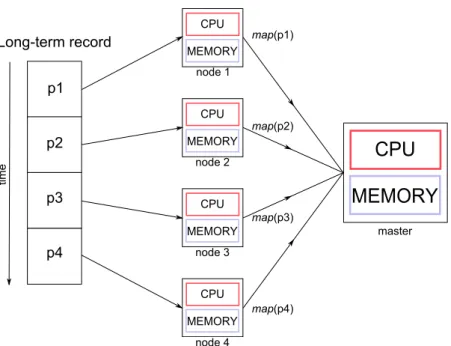
CPU MEMORY CPU MEMORY CPU MEMORY CPU MEMORY node 1 node 2 node 3 node 4 map(p4) map(p3) map(p2) map(p1) p1 p2 p3 p4 Long-term record time

Figure 3.2: Schematic of the whole computation. In this situation the division of the long-term record gives rise to 4 data-structures, which are processed in 4 computing nodes, prior to the application of thereducefunction by the master computer.

the fastest way to compute these parameters might be in a distributed manner, due to the size of the biosignal (as was mentioned in chapter 2, these parameters might also be computed by a single processor, sequentially, analysing each part at a time). Thestandard deviation,histogramandevents detectionMapReduce algorithms will be presented.

3.3.1 Histogram and pNN50

The histogram of a signal is a tool meant for the analysis of the amplitude distribution of the signal samples. Before the computation of the histogram, the number of bins is de-fined. The bin size will be equal to the amplitude of the signal divided by the number of bins. Sometimes it is only relevant to know the distribution of the signal values between a certain interval, dismissing the samples outside the interval. If so, the maximum and minimum values of the signal do not need to be known beforehand and the bin size will be equal to the interval size divided by the number of bins. In this section the histogram is only meant as the information necessary to compute the graphical representation of this analysis tool and not the figure itself. Thehistfunction might be defined as follows:

hist(X, nBins) = ((i1, i2, . . . , inBins),(c1, c2, . . . , cnBins)), (3.10)

(45)

IfX =x1, x2, . . . , x_n, themapfunction is simply:

histM ap(x, nBins) =hist(x, nBins) (3.11)

The associatedreducefunction is:

histReduce(m1, m2, . . . , mn) = m1[0],

n

X

i=1

mi[1]

!

, (3.12)

wheremiare the mapping results, i.e, the outputs of thehistM apfunction.

Each node computes partial histograms and the reduce function simply adds up the counts from all the different parts.

The pNN50, a widely used HRV analysis parameter can be computed following this process, since the problem involves counting events. The NN50 is the number of interval differences of successive RR intervals greater than 50 ms. The pNN50 is obtained divid-ing NN50 by the total number of RR intervals. A detected regularity in large changes in successive RR intervals may indicate cardiac parasympathetic damage [24].

Because of the mathematical complexity of the pNN50 MapReduce algorithm, only a description of the steps taken by themapandreducefunctions will be made.

For the computation of this parameter, themapfunction would need to return:

• The number of successive RR intervals spaced by more than 50 ms;

• The number of RR intervals computed in that signal part (equal to the total number of detected ECG peaks less 1);

• The order in which the signal slice appeared in the long-record (this has to be an ar-gument of the map function, passed by the master computer when assigning tasks to the computing nodes);

• The first and last detected peak and the first and last RR interval.

The reduce function would first compute the NN50 parameter. For that, it would:

1. Sort all the mapping results according to the order of the slice they refer to in the original record;

2. Compute the lost RR intervals in the borders of the slices. For that it uses the first peak of a mapping result and the last peak of the previous mapping result and compares the resulting RR interval with the adjacent intervals evaluating if they are spaced by more than 50 ms;

3. Sum all the partial NN50 mapping results and the ones found out in 2., obtaining the NN50 parameter.

(46)

3.3.2 Standard deviation

When aiming to write the parallel version of a simple mathematical calculation it is best to fully understand the definition of the parameter. The standard deviation is computed as shown in the following equation:

std(X) =pE[X2_]₋₍_E_[_X_])2_, _(3.13)

whereE[X]is the mean value ofX. LetX ={x1, x2, . . . , x_n}. In this case the division

of X gives rise to n partitions. The standard deviation map function applied to each partition is

stdM ap(x) = (sum(x2

), sum(x), length(x))∈R3 _(3.14)

Before presenting the associatedreducefunction it is important to appreciate the size reduction that happened during the mapping process. Initially the standard deviation could not be computed by a single processor, due to memory issues because of the size of the signal. After the mapping process, each signal part "is" reduced to a 3 element tuple. Provided that all the necessary information for the final computation is within that tuple, the master computer will have no trouble (memory-wise) computing the parameter.

The standard deviationreducefunction will have a number of arguments equal to the number of partitions. Letmn = stdM ap(xn)ands =sum(m1, m2, . . . , m_n), i.e.,sis the

sum of all the mapping tuple results element-wise. Then, the standard deviationreduce

function is:

stdReduce(m1, m2, . . . , mn) =

s

s[0] s[2] −

s[1] s[2]

2

(3.15)

It is easy to verify that equation3.15is correct according to the definition (equation

3.13), since:

• s[0] =P

X2

• s[1] =P

X

• s[2] =length(X)

3.3.3 Events detection

(47)

• a ECG peak detection algorithm (or QRS detector as it is sometimes referred to);

• a respiratory cycles detection algorithm, which allow the computation of the breath frequency from respiratory signals;

• an algorithm for the detection of muscle activity from a EMG record.

These examples are just a sample of the applications of events detection algorithms. Thus the importance of the suitability of these kind of algorithms to run in parallel, which will drastically reduce their execution times. The division of the signal will typically be accompanied of an overlapping portion, since the events detection algorithms do not perform the same in the edges as in the middle of the signal.

In this work, two events detection algorithms were used (although more loosely one could also consider the computation of the pNN50 parameter and the histogram as events detection algorithms): a ECG peak detection algorithm, fundamental for the de-veloped HRV analysis tool and a respiratory cycles detector, just as important, regarding a respiratory analysis tool (these tools will be described in the next chapter).

Themapfunction utilized in this class of algorithms is basically the events detection algorithm itself. The computing nodes will search for events over the signal slices that were assigned to them and return the detected events and the order in which their signal slice appeared in the original signal.

Thereducefunction will only have to sort the mapping results (assuming the instant or time interval of the detection is important - it may only matter that an event was detected) and possibly remove some double detections. Double detections might occur due to the detection of the same event in an overlapping region and in the edge of the subsequent partition.

Executing this class of algorithms in a distributed environment has a huge poten-tial, since the speedup factor is approximately proportional to the number of computing nodes. A biosignal of about 7 hours, acquired during the night can be partitioned in time slices that are smaller and smaller, as more and more computing nodes are assigned to the problem. If the algorithm performs well over slices of a few seconds, there is nothing preventing the problem to be solved in approximately that amount of time, provided that enough computing power is available.

Generally, for this type of problems the execution time is:

T =map time+reduce time (3.16)

Assuming that the signal slices are equally sized,

map time≈ sequential time

number of partitions (3.17)

(48)

time).

The overall execution time becomes:

T ≈ sequential time

number of partitions +reduce time (3.18)

This is the reason why thereducefunction must do as little work as possible and we must load the working nodes as much as possible: themaptime can be reduced by further dividing the signal, but the speedup will always be limited by the execution time of the

(49)

4

Signal processing tools

4.1 Overview

In this chapter, two signal processing tools developed during this work are described. These processing modules were integrated in a long-term biosignals visualization tool, a result of a previous work [16]. The resulting tool allows the clinician and the researcher to analyse long-term records without having to deal with all the programming and sig-nal processing algorithms directly. An effort was made to asig-nalyse long-term records efficiently. In this context, parallel programming techniques came naturally as a way to solve possible bottlenecks that limit the speed at which the signals are processed.

In the next section, the acquisition system is described. Then, the programming ar-chitecture of the proposed application and two biosignal analysis tools - a heart rate vari-ability analysis tool and a respiratory analysis tool - are presented, as well as some of their applications.

4.2 Acquisition system

To acquire long-term biosignals is no easy task. The acquisition system must be as com-fortable as possible, so that the patients are not disturbed by its utilization. This par-ticular study occurred under the project "wiCardioResp" [4]. This project is developing technology to remotely monitor patients with cardiorespiratory problems and neuromus-cular diseases (such as amyotrophic lateral sclerosis) while the patients are comfortably at home. The acquisitions were carried out with the patients agreement, during the night, and last approximately 7 hours.

(50)

4. SIGNAL PROCESSING TOOLS 4.3. Application architecture

wrap, which integrates respiration, ECG and accelerometer sensors (see figure4.1). The sensors were provided by PLUX, Wireless Biosignals, S.A..

The chest wrap makes it harder for the sensors to detach from the patient due to sleep movements, which would compromise the acquisition.

Figure 4.1: Chest wrap with integrated accelerometer, ECG and respiration sensors.

The applications of the analysis of heart rate variability and the analysis of respira-tory signals were mentioned in chapter2. The accelerometry signals make it possible to identify sleep periods in which the patient turned over in bed.

The signals were sampled at 1 kHz and with a 12 bit resolution. They were sent by Bluetooth to a mobile phone and recorded in *.txt format.

4.3 Application architecture

As mentioned, the signal processing tools developed were integrated in a pre-existing tool. A schematic of the architecture of the application is depicted in figure4.2.

4.3.1 Previously developed work

The tool has a visualization module, developed in a previous work [16], which allows the visual inspection of very long signals. Signals approximately 7 hours long, and sampled at 1 kHz are composed by millions of samples.

First there is a conversion step, in which the *.txt recorded signals are converted to the hdf5 file format, with the advantages mentioned in chapter2.

(51)

4. SIGNAL PROCESSING TOOLS 4.3. Application architecture

Figure 4.2: Programming architecture of the signal processing tool.

would vary in detail depending on the time length one would wish to visualize. The keys ’+’ and ’-’ allow zoom in and zoom out respectively. An example of a 7 hour long ECG record is show in figure4.3.

2h44m28.2s 4h6m42.2s 5h28m56.3s 0.24V 5.00V

Figure 4.3: Multilevel visualization of a 7 hour long ECG

The tool runs in a web browser, rendering it extremely portable and giving it the potential to be accessed from anywhere with an internet connection. The signals can ultimately be stored in a server and accessed remotely from anywhere through the appli-cation and the signal processing can happen remotely.

4.3.2 Newly developed work

The signal processing modules were integrated in the application as depicted in figure

(52)

4. SIGNAL PROCESSING TOOLS 4.4. Heart rate variability analysis tool

originating websocket requests. These requests typically include:

• The name and directory of the signal file;

• The channel of the signal (the records contain several types of signals, each one from a different channel in the recording device);

• The initial and final time of the signal slice the user is currently viewing;

• The name of a function (a processing function), which is associated to the action the user triggered on the browser.

All this is hidden from the user and is already associated to interactive elements such as buttons or dragging elements. Any further information related to the signal, which might become necessary in the signal processing algorithms is obtained by accessing the file and reading the corresponding metadata (hdf5 attributes).

So, for example, there might be a button that "computed" the mean of a portion of the signal. The user would press that button, and automatically the information described above would be sent through the websocket and be the input of ameanalgorithm (which might be implemented in parallel). The result would then be sent back through the web-socket to be displayed to the user in the browser.

The processing result (such as plot or parameters) are displayed next to the visual-ization of the signal and allow a direct interaction with the signal, as will be explained next.

4.4 Heart rate variability analysis tool

All heart rate variability analysis algorithms are based on the RR intervals. Other than the spacing between all QRS complexes, the values the ECG assumes are completely meaningless in HRV analysis.

A signal lasting 7 hours and sampled at 1 kHz has 25.2 millions of samples. However, the number of RR intervals in the signal is relatively small, and independent from the sampling frequency. Considering a mean heart rate of 60 beats per minute, the number of RR intervals would be 25199, about 1000 times smaller than the length of the signal.

If the user selects the first three hours of the signal, and wishes to see the tachogram (RR evolution in time) those three hours of the signal would have to be processed, start-ing at the detection of the R peaks. Only then could the HRV processstart-ing algorithms be applied.

Processing the ECG this way, every time the user makes a request, is a tedious process (see chapter5for the detailed execution times) and not at all practical.

(53)

The ECG peak detection step is always the first step of the analysis and is applied over the whole signal, regardless of the time slice the user wishes to view. This process only has to be done once. The results are stored in a *.h5 file, and are accessed every time the user makes a request related to the associated ECG record. This introduces an interesting concept: storing meaningful processing results which are necessary for further analysis, to spare time in future analysis sessions. Now, if the user selects a 3 hour time slice, the *.h5 file containing the instants of the different R peaks is accessed and the peaks corresponding to the selected time slice are extracted right away to be used by HRV analysis algorithms. This process is illustrated in figure4.4.

0.388 1.309 2.238 3.132 3.931 4.728

0.850 4.430

All RR intervals (s): (0.921, 0.929, 0.894, 0.799, 0.797)

Selected RR intervals (s): (0.929, 0.894, 0.799)

Figure 4.4: The user only wishes to analyse the portion of the signal between the dashed lines (0.85 s to 4.43 s). Of the 6 total peaks, only 4 of them are retrieved and 3 RR intervals are computed (out of the total 5).

The red dots in figure4.4are the detections of the ECG peak detection algorithm. For a matter of simplicity, only a small signal is shown, but the same principle applies to any other signal.

This preprocessing step is executed in parallel and its execution times are discussed in chapter5. By waiting a few minutes for the preprocessing step to complete, a huge amount of time is saved in the future. The heart rate variability tool provides analysis results in just a few seconds (less than 10 seconds) and can in this sense be classified as a real-time analysis tool.

(54)

In a future session, when the user loads the signal, the program looks for the process-ing results file and the peak detection is skipped.

An overall view of the integration of the processing module in the visualization tool is illustrated by figure4.5

Visualization Tool Signal Processing Tool 1 2 3

Figure 4.5: 1. Report Generation; 2. Programming mode analysis; 3. On-screen analysis.

The signal processing tool has 3 main functionalities: the on-screen analysis, a report generation feature and a programming mode analysis.

4.4.1 On-screen analysis

The on-screen analysis, as the name suggests, is displayed in the browser. After all the HRV analysis algorithms execute, the results are sent through the websocket and prop-erly displayed. The results may be visual representations (plots) or tables with parame-ters relevant to the analysis. The on-screen analysis was organized in 3 different groups: (linear) time domain analysis, frequency domain analysis and non-linear analysis. In figure 4.5 only the container elements of the time and frequency domain analysis are displayed. The grey tabs allow the user to switch between the different results easily.

The on-screen analysis results of a 7 hours long ECG are illustrated in figure4.6. All the parameters and visual representations were computed according to [21].

(55)

Ricardo Daniel Domingos Chorão