Modelling of a lens antenna receiver system for NASA GUSTO

(1)

Ricardo de Araújo Farinha

Bachelor in Micro and Nanotechnologies

Modelling of a lens antenna receiver system for

NASA GUSTO

Dissertation submitted in partial fulfillment of the requirements for the degree of

Master of Science in

Micro and Nanotechnologies Engineering

Adviser: Dr. J. R. Gao, Senior Instrument Scientist, Department of Quantum NanoScience Delft University of Technology

Co-adviser: Dr. Luís Pereira, Associate

Professor, Faculty of Sciences and Technology New University of Lisbon

Examination Committee Chairperson: Dr. Rodrigo Martins

Raporteurs: Dr. João Goes Dr. J. R. Gao

(2)

(3)

Modelling of a lens antenna receiver system for NASA GUSTO

The Faculty of Sciences and Technology and the NOVA University of Lisbon have the right, perpetual and without geographical boundaries, to file and publish this disserta-tion through printed copies reproduced on paper or on digital form, or by any other means known or that may be invented, and to disseminate through scientific reposito-ries and admit its copying and distribution for non-commercial, educational or research purposes, as long as credit is given to the author and editor.

This document was created using the (pdf)LA_{TEX processor, based in the “unlthesis” template[1], developed at the Dep. Informática of FCT-NOVA [2].}

(4)

(5)

(6)

(7)

Acknowledgements

Every person here mentioned contributed in some way to make this moment happen. I would like to first tank to my supervisor Dr. J.R. Gao of TUDelft from TUDelft/S-RON, for making it possible for me to research in his field and welcoming me in open arms in a foreign country. He has always inspiring, supportive, dedicated, and even tough always busy with some project, he always made time for me. Thank you for everything. To my co-supervisor Prof. Dr. Luís Pereira from FCT/UNL, for his knowledge and help over the years.

To Darren Hayton from SRON, thanks you for your help during my measurements and by showing how to deal with problems. To Benham Mirzaei from TUDelft, for his help during the meetings and for teaching me to ask everything. To Geert Keizer from SRON for using his time helping in my measurements. Ao Zé Rui, por me oferecer o chão da casa quando precisei e por ser como um irmão na Holanda.

To Erasmus plus for supporting me financially.

Ao Prof. Dr. Rodrigo Martins e à Prof. Dra. Elvira Fortunato pela criação e promoção do curso de Engenharia Micro e Nanotechnologias.

Aos meus pais por me criarem e por estarem presentes sempre que precisei. À minha mãe por me por juízo na cabeça e ao meu pai por toda a magia.

Ao meu irmão por me fazer me rasteiras, bater me e quase cegar me em lutas de areia. Mas também, por me ter sempre apoiado em projetos malucos.

À minah avó poque para além de ser chata, me deixava comer colheres gigantes de maionese no bacalhau à braz.

A toda a minha família por todos os jantares de Natal.

À Sofia aos momentos que passamos, sejam festas, a ressacas, viajens pela europa, a dormir um dia inteiro, pelos drifts às comidas que engordam 1 kilo por garfada, dos jantares, às séries e filmes, estejamos longe ou perto, mudaste a minha vida. A faculdade nao teria sido a mesma coisa sem ti. Obrigado!

Ao Migas pela formiga Tobias, aos jogos de FIFA, às lans parties e ao bulling.

Ao Ribas e ao Gonçalo por todas as viagens, pelas festas, pelos jogos e pela amizade. Já com 50 anos ainda vamos estar a tentar chegar a global.

Ao mágico por todas as broculices e fadas.

Ao Ramos e ao Minhoca por serem os meus padrinhos não oficiais e me ajudarem sempre que precisei.

À noiva dourada que um dia vou casar realmente depois de uma bebedeira, só porque podemos. Pelo riso de ganso, pelo oásis no deserto e pelos anos de parvoíces que temos pela frente.

À Filipa e à Andreia por mostrarem o lado wild da vida.

Ao Ismael pela nação CROISSANT e pelo nosso momento romântico na lagoa de Albufeira.

À Erica, à Inês e à Trapula pelas saídas, pelos minions, pelas férias e pela amizade.

(8)

À Inês por me alimentares e me arrancares pêlos.

Ao Jaime, ao Almeida e ao Gabriel pelos fritanços na 202.

To Giordano and Guilhem for the barbecues, drinks and friendship.

To all the people from the MIEMN course and to many other people that I surely forgot to mention, but that helped me be who I’m today. Thank You, Obrigado.

(9)

Abstract

The radiation at terahertz (THz) frequency range (1 THz = 300 µm in wavelength) provides us a powerful window into cosmic evolution, from the birth and explosion of stars to the evolution of galaxies and the universe itself. The THz is a largely unexplored region in the electro-magnetic spectrum, partly owing to technological constraints and partly due to atmospheric absorption on the Earth. Consequently, THz astronomy ob-servations are best performed from space-based or balloon-borne telescopes, like the proposed NASA balloon GUSTO mission. The observations will be complementary to other space missions like Hershel’s HIFI instrument.

In this work, a model of GUSTO’s optical system was proposed and analysed in order to improve its efficiency in detecting three of the most important terahertz lines, [NII], [CII] and [OI], with multi-pixel heterodyne cameras. Moreover, simulations were per-formed with PILRAP, a antenna simulation software, to study the parameters that affect the optical f# number and radiation pattern of a 5 mm diameter lens system, and to explain the heterodyne sensitivity diff_{erences between a 10 mm lens and 3.1 mm lenses.} Outcome of my thesis work concludes the feasibility to use smaller lens for GUSTO’s heterodyne arrays.

Keywords: GUSTO, THz, HEB, Optic Design, Lens Design, PILRAP

(10)

(11)

Resumo

A radiação com frequência na faixa dos terahertz (1 THz = 300 µm de comprimento de onda) proporciona-nos uma poderosa janela para a evolução cósmica, desde o nasci-mento à explosão de estrelas, até à evolução de galáxias e do próprio universo. O THz é uma região inexplorada do espectro electromagnético, em parte devido a restrições tecnológicas e em parte devido à absorção atmosférica na Terra. Consequentemente, a melhor forma de realizar as observações astronómicas em THz é a partir de telescópios, espaciais ou a bordo de balões, como a missão GUSTO proposta à NASA. As observações serão complementares de outras missões espaciais como o instrumento HIFI do Hershel. Neste trabalho, foi proposto e analisado um modelo do sistema ótico do GUSTO, a fim de melhorar a sua eficiência na detecção de três das linhas terahertz mais importantes, [NII], [CII] e [OI], com câmaras heteródinas multi-pixel. Além disso, foram feitas simu-lações com o PILRAP, um software de simulação de antenas, para estudar os parâmetros que afectam o número f# óptico e o padrão de radiação de um sistema de lentes com 5 mm de diâmetro, e explicar as diferenças de sensibilidade heteródino entre uma lente de 10 mm e lentes de 3.1 mm. O resultado da minha tese conclui a viabilidade de usar lente mais pequena para as matrizes heteródinas do GUSTO.

Palavras-chave: GUSTO, THz, HEB, Design Ótico, Design de Lentes, PILRAP

(12)

(13)

List of Figures

1.1 Life cycle of the Interstellar Medium (ISM), from warm neutral clouds cooling down and assembling together forming giant molecular clouds, to the forma-tion of stars destroying the molecular clouds. The ions marked in yellow, allow for the full probe of the ISM, becoming the main focus of this thesis. Adapted from [6]. . . 1

1.2 Heterodyne receiver system. The two signals are merged and coupled into the mixer, and the output, the Intermediate Frequency (IF) signal is then ampli-fied, filtered and recorded. Adapted from [20]. . . 3

1.3 a) Hotspot model of HEB mixing. The Astronomical Signal (AS) + Local Os-cillator (LO) power is conveyed to the resistance modulation of the HEB at IF frequency. b) HEB I–V curve. Incident RF (i.e., LO) power will acelerate the transition, reducing the amount of current that can flow through the device at a given bias voltage[21]. . . 4

1.4 3D model of Galactic/Xgalactic Ultra long duration balloon Spectroscopic Stratospheric THz Observatory (GUSTO) telescope . . . 5

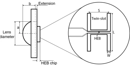
2.1 Lens with superconductor Hot Electron Bolometer (HEB) chip showing the dimension related parameters. The extension of the lens plus the HEB chip thickness defines the extension length used in Program for Integrated Lens and Reflector Antenna Properties (PILRAP). . . 8

3.1 Original GUSTO Instrument Block Diagram proposed to NASA, with 3x8 cooled HEB receivers. The colors show the organization responsible for the component.. . . 9

3.2 New proposed design for the GUSTO balloon with outside cryostat optics and dichroic filters working as beamsplitters. . . 11

3.3 Christopher Walker’s new design, with outside optics and the Quantum Cas-cade Laser (QCL) inside the cryostat. A QCL frequency lock loop is introduced to stabilise the QCL frequency.. . . 15

3.4 Most favourable design, with telescope beam directly to [OI] channel detectors and with less optical components. . . 15

3.5 Power beam pattern of 5 mm lens and antennas at 1.4 THz, 1.9 THz and 4.7THz. 18

3.6 Contour of the efficiency and the optical f# of a lens-antenna systemas a

func-tion of the lens extension length and ellipticity. . . 19

3.7 Optical f# of the lens-antenna as a function of the efficiency . . . 19

3.8 Receiver noise temperature measurement in the vacuum setup for one 10 mm diameter lens and three 3.1 mm diameter lenses. L1 was measured with a ticker beamsplitter (BS), so based on the results of of L2 and L3, L1 was corrected to allow comparisons. [39] . . . 20

(16)

L i s t o f F i g u r e s

3.9 Comparison between noise temperature measurements in air setup vs vacuum setup in both 10 mm diameter lens and one 3.1 mm lens (L1) [39]. . . 21

3.10 Total lens efficiency as a function of the extension length and the relative

dielectric constant. . . 22

3.11 Efficiency as a function of extension length, assuming a relative dielectric

constant of 11.4. . . 22

3.12 Efficiency as a function of the dielectric constant for 0.514 mm extension

length and 0.482 mm. . . 23

3.13 a) Coordinate Measuring Machine (CMM) used to measure the lens dimen-sions. b) 3.1 mm lens strapped between two clamps. . . 24

3.14 Efficiency as a function of the variation from the optimum extension length for

each lens. Marked in circles is the difference between the optimum extension

and the optical extension measured for the four lens. . . 26

3.15 Efficiency as a function of the relative dielectric constant, using the simulation

results with the optical measured dimensions of the lenses. . . 27

A.1 Simulation of a dichroic filter that can be used as a beamsplitter for 1.46 THz, while transmitting at 1.9 THz. . . 35

B.1 All optical designs tested, with f) being the preferred one. . . 37

C.1 All optical designs tested, with a) being the preferred one. . . 39

(17)

List of Tables

1.1 State-of-the-art of GUSTO complementary missions. . . 6

3.1 Optical losses associated with all optic components of GUSTO . . . 12

3.2 Optical losses calculation results and their differences. . . 12

3.3 LO power required for normal HEB operation. . . 13

3.4 Optical losses calculation results for the two new designs and their differences. 16 3.5 LO power required for the two new designs for normal HEB operation. Both designs have the same LO signal. . . 16

3.6 Parameters used for the 5 mm lens simulation. . . 17

3.7 Simulation results of the 5 mm lens. . . 17

3.8 Simulation parameters for the optimisation of the f#. . . 18

3.9 Values used for each parameter in the simulation program PILRAP. . . 21

3.10 Results of the lens height measurements compared to the expected design dimensions. . . 25

3.11 Extension length without the substrate thickness for the optical measurement. It also shows the distance from optimum extension, simulated in PILRAP. . 25

(18)

(19)

Glossary

Cooper pairs is a pair of electrons (or other fermions) bound together at low

tempera-tures, responsible for the peculiar properties of superconductivity .

Noise temperature is the equivalent temperature to the noise power introduced by a

component or source, that ultimately determines the sensitivity of the receiver sys-tem .

(20)

(21)

Acronyms

AS Astronomical Signal.

BICE Balloon-borne Infrared Carbon Explorer.

CMM Coordinate Measuring Machine.

COBE Cosmic Background Explorer.

FIR Far-infrared.

FIRAS Far InfraRed Absolute Spectrophotometer.

FWHM Full Width at Half Maximum.

GREAT/SOFIA German REceiver for Astronomy at Terahertz / Stratospheric

Observa-tory for Infrared Astronomy.

GUSTO Galactic/Xgalactic Ultra long duration balloon Spectroscopic Stratospheric THz

Observatory.

HEB superconductor Hot Electron Bolometer.

HIFI Heterodyne Instrument for the Far-Infrared.

IF Intermediate Frequency.

ISM Interstellar Medium.

KID Kinetic Inductance Detector.

LMC Large Magellanic Cloud.

LO Local Oscillator.

PILRAP Program for Integrated Lens and Reflector Antenna Properties.

QCL Quantum Cascade Laser.

SIS Superconductor-Insulator-Superconductor tunnel junction.

STO Stratospheric Terahertz Observatory.

TES Transition Edge Sensor.

THz Terahertz.

(22)

(23)

Symbols

Bν Intensity of ligth emitted from the blackbody

dΩ Solid angle

f# f-number

LB Bridge length

LH Hotspot length

I_C Critical current

NbN Niobium Nitrade

PLO LO power

T_B Bath temperature

TC Critical temperature

VB Bias Voltage

[CII] Ionized carbonC+

[NII] Ionized nitrogenN+

[OI] Neutral Oxygen

ǫ_r relative dielectric constant

ν Frequency

θ Azimuth angle

φ Zenith angle

ηtotal Total efficiency

ηs Spillover efficiency

ηtr Transmission efficiency

ηa Aperture efficiency

η_p Polarisation effi_ciency

(24)

(25)

Motivation

The first stars were created about 13.7 billion years ago from light elements such as hydrogen, helium and lithium. By nuclear fusion, heavier elements are created like carbon, nitrogen and oxygen, forged in the interior of stars. Billions of years later, these stars turn unstable, collapsing and exploding, scattering all these elements as floating stardust.

The atoms that comprise life on Earth, the atoms that make up the human body, all come from exploding stars. We are made from stardust, and probably the atoms from our right hand came from a different star than the ones from our left hand. (Lawrence M. Krauss and Neil deGrasse Tyson)

At some point in life, every person probably wonders about two fundamental ques-tions:

• Are we alone in the Universe?

• Where we all came from?

This work may not contribute to the first question, but by studying the birth and death of stars to the evolution of galaxies, maybe, we will be a tiny fraction closer to a solution to the second question, and that is worth pursuing.

It costs around 9000 euros per kilo to launch cargo to the space station. Making things smaller and lighter is, therefore, a natural route to reducing the cost of launching a spacecraft. Nanotechnology can bring a multi-planetary future to reality, but there is long journey ahead. This thesis work allows me to conciliate my deep interest for space and nanotechnology, and be part of the exploration of the cosmos.

(26)

(27)

Objectives

Heterodyne receiver technology is the key technology to observe astronomic fine struc-ture lines, crucial to understand the life-cycle of starts and planets. To map the line in our galaxy or nearby galaxies, an array receiver with a high spectral resolution, is required. Such an array receiver is demanded for a planned NASA suborbital balloon telescope GUSTO. However, it only became possible to build through recent technologi-cal advances. Although this increases scientific throughput and reduces the cost, it adds complexity to the optical system. Efficiently capturing, conveying, and analysing this light is the purpose of all astronomical instrumentation.

This project aims to:

1. Understand the astronomic requirements and instrument concept of GUSTO;

2. Study and improve GUSTO optical system;

3. Simulate lens to optimise its optical f# number;

4. Simulate lens characteristics to explain experimental noise temperature data.

Work structure

The work is organised as following:

Chapter 1 will introduce to the concept of THz astronomy, describing the importance of heterodyne systems, while explaining HEB’s theory of operation, the optical system and coupling of THz signals. It ends with a brief description of the GUSTO balloon and a state-of-the-art based on previous and current space missions.

Chapter 2 will describe all the fundamental proprieties to explain the principle of coupling mixers and the parameters necessary to simulate a lens/antenna system with PILRAP.

Chapter 3 is divided in four main parts: two regarding GUSTO’s optical system design and the other two for lenses simulation. The first part of optical design tries to improve a design from the original proposal. At the same time, Christopher Walker, Principal Investigator of the GUSTO project, designed a new optical system. Hence, the second part tries to improve this new design. The first part of the lenses simulations are focused in decreasing the optical f# number of a 5 mm lens, while the second part focus in explaining the noise temperature measured by a master thesis student José Silva.

Chapter 4 will summarise the results and describe the next steps for the project. This will be followed by the Appendix and Annex sections for additional information.

(28)

(29)

C h a p t e r

1

Introduction

1.1 Terahertz Astronomy

TheTerahertz (THz)frequency range, also known as the sub-millimeter andFar-infrared (FIR)range, is loosely defined as the frequencies between 0.3 THz to 10 THz, or the wave-length from 30 µm to 1 mm [1, 2]. In the last decade, an advance inTHztechnologies raised the potential for new applications in astronomy, medicine, security, communica-tions, and material identification [1].

This frequency range is perhaps the final largely-unexplored spectrum region and the least developed, partially owing to the diffi_{culty in constructing}_THz_{sources, detectors} and transmission devices, and due to the radiation absorption of Earth atmosphere [3]. H2O, O2, and O3are highly efficient absorbers of photons at this frequency [4,5]. The

higher the altitude, the lower is the density of these elements. Therefore,THzastronomy observations are best performed from space-based telescopes, balloon-borne telescopes, airborne observatories or at high, dry, and cold sites on Earth, like Antarctica [4].

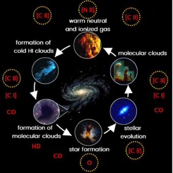
Figure 1.1: Life cycle of theISM, from warm neutral clouds cooling down and assembling together forming giant molecular clouds, to the formation of stars destroying the molecu-lar clouds. The ions marked in yellow, allow for the full probe of the ISM, becoming the main focus of this thesis. Adapted from [6].

In astronomy, THzradiation is important to probe the Interstellar Medium (ISM), composed of gas and dust between the stars, yielding valuable insights into star formation and the life cycle of interstellar clouds, seen in Figure 1.1. Photons being emitted by

(30)

C H A P T E R 1 . I N T R O D U C T I O N

clouds have relatively larger wavelengths (~100-1000 µm) compared to interstellar dust grains (~0.1 µm), and consequently, are less affected than UV, visible and even IR light [7].

The ISM is composed by multiple phases, distinguished whether matter is ionic, atomic, or molecular and by the temperature and pressure of the clouds [8]. At each phase of theISMcycle, different ions will emit at different frequencies in theTHzrange. The three most important emission lines studied in this project are the nitrogen [NII] at 1.46 THz, carbon, [CII] at 1.90 THz, and oxygen, [OI] at 4.75 THz. [CII] line is associated with all phases of theISM, [NII] arises from the ionised regions, allowing to distinguish neutral from ionised gas clouds, and [OI] emission is linked to the formation of stars [7].

After half a century of study, key questions about theISMremain: where and how are interstellar clouds made? Under what conditions and at what rate do clouds form star? And how do these processes sculpt the evolution of galaxies? [9]

1.2 Direct and heterodyne terahertz detectors

THzdetection technology can be divided in two main groups: heterodyne (coherent) detection systems, which allows detection of amplitude and phase of a signal, and di-rect (incoherent) detection, which only allows amplitude detection of the signal. The most common direct sensors are theTransition Edge Sensor (TES)[10] and theKinetic Inductance Detector (KID)[11], while for the heterodyne sensors it’s the Superconductor-Insulator-Superconductor tunnel junction (SIS)[12,13] and thesuperconductor Hot Elec-tron Bolometer(HEB) [14–16].

At the centre of the galaxy, rotational velocity of the stars is much higher, and due to the Doppler effect, the detected signal’s frequency shifts (e.g. an ambulance siren sounds higher in pitch when it is approaching than when it is receding). Only the hetero-dyne detectors can offer high spectral resolution and sensitivity capable of resolvingTHz emission and/or absorption lines to distinguish the emitting clouds [17].

TheHEBsbecome the heterodyne detector of choice for frequencies above 1.5 THz sinceSISmixers work only up to this frequency, due to their mixing principle and to the superconducting gap of available materials [2,3,18].

1.3 Superconducting Hot Electron Bolometer

A heterodyne receiver converts anAstronomical Signal (AS) of high frequency into a signal with lower frequency (several GHz), where it can be amplified and processed. The down conversion is achieved by multiplying the incoming astronomical light with a locally produced signal, calledLocal Oscillator(LO), a continuous wave with extremely stable frequency or phase. This multiplication occurs in a device called mixer, as seen in Figure1.2. The output signal it’s calledIntermediate Frequency(IF), and it’s a copy of the astrophysical spectrum, but converted to the GHz frequency range [19].

(31)

1 . 3 . S U P E R C O N D U C T I N G H O T E L E C T R O N B O L O M E T E R

Figure 1.2: Heterodyne receiver system. The two signals are merged and coupled into the mixer, and the output, theIFsignal is then amplified, filtered and recorded. Adapted from [20].

For this project,HEBs are the mixer of choice, thermal devices in which the resistance depends on the temperature [18]. They are formed by a short (∼200 nm), thin (∼5 nm),

superconducting niobium nitride (NbN) bridge between two normal (e.g. gold) electrodes [21].

For theLO, there are two types used for this project: frequency multiplierLOand

QCL. The multiplier works from 0.1 to 2.7 THz and is based on the multiplication of a GHz signal, however, their output power decreases exponentially with frequency [22]. TheQCLhas been demonstrated at 4.7 THz, important for the [OI] line, and it’s based on the ‘intersubband’ transitions in a repeated stack of semiconductor quantum wells [23].

Figure1.3(a)shows the theory of operation. The input andLOsignals are conveyed to anHEB, either quasi-optically or via waveguide, and enter the bridge through contact pads. At zero bias voltage (V_B= 0 V) theHEB behaves as a short circuit, seen in Figure

1.3(b). AsVBincreases (either in the positive or negative direction),Cooper pairswithin the bridge begin to break and the device no longer behaves as a pure superconductor. TheHEBcurrent,IB, initially remains constant and then begins to increase as the bridge transitions to being a normal resistor. The HEB is biased so that the combination of DC bias, LOpower, and bath temperature (T_B= 4 K) place it on a nonlinear transition between a normal and superconducting state. In this transition region, the central part of the bridge is heated to its critical temperature,T_c, and driven normal, while adjacent ends of the bridge remain superconducting. The region of the bridge that is driven normal is referred to as the “hotspot", with lengthLH[21].

TheLOand theASwill modulate the length of the "hotspot". It is this modulation that yields the downconverted signal that is passed into a low-noise IF amplifier. The maximum IF frequency supported by the HEB is determined by how fast heat can be transferred out of the bridge, either by electron diff_{usion through the contact pads at} the ends or by electron-phonon coupling to the crystal lattice in the substrate material.

GUSTOwill choose the latter. [21].

(32)

(a) (b)

Figure 1.3: a) Hotspot model of HEB mixing. The AS+ LO power is conveyed to the resistance modulation of the HEB at IF frequency. b) HEB I–V curve. Incident RF (i.e., LO) power will acelerate the transition, reducing the amount of current that can flow through the device at a given bias voltage[21].

1.4 Terahertz Optics

To efficiently capture, convey and analyse the terahertz light, the astronomical instrument guides the light to a detection system [24]. Lenses and/or mirrors are used to accomplish this, with each of these having their advantages and disadvantages. The lenses are more lossy than the mirrors, due to absorption and reflection of the dielectric material, but they are more compact. Often the best solution is a hybrid approach [24].

A common component is the dielectric beamsplitter. Instead of trying to achieve 100% reflectivity or transmissivity, it has a ratio of transmitted and reflected power, for example a 90/10 ratio is usually used to combine theLOlaser and the incoming beam from space. For polarised light, a wire grid polariser splits the incoming light into two, depending on its polarisation. The vertically polarised photons go in one direction while horizontally polarised photons go to another [24].

To separate or merge the incoming beam of light into different frequencies, a dichroic filter is used. These are periodically perforated components, where the shape and ar-rangements of the apertures is determined by the filter characteristics [25]. These filters have a diff_{erent transmission and reflection coe}ffi_{cients for di}ff_{erent frequency ranges} [26].

When designing a heterodyne array, while for a multiple-LO, the baseline source is the same for all the pixels, meaning they emit the same frequency, having multiple sources would mean a different frequency for different pixels.The Fourier Phase Grating is a reflective grating that splits a beam into a given number of equally beams, being an efficient way to distribute the power of aQCL. This is possible due to the use of periodic structures (cells) on its surface based on the Fourier series expansion theory. This way

(33)

1 . 5 . BA L L O O N G U S T O

each pixel will be operated at the sameLOfrequency [27].

To intercept the Gaussian beam an open structure (quasi-optical) detection system is preferred, e.g. is shown in Fig2.1. A lens focus the incoming light into an absorbing layer, on which is mounted one or more broadband detectors. TheTHzdetector is much smaller than the wavelength being received. Therefore, a planar antenna structure, typically a twin-slot or a spiral, and associated coupling circuitry are needed to bring the radiation to the detector [3]. Spiral antennas operate with circular polarised ligth and a broad RF bandwidth, while twin-slot antennas operate linear polarised ligth, with acceptable beam pattern [18]. For practical reasons, the spiral antenna is preferred, since there are no problems with aligning the polarisation and with the broad RF bandwidth,the instrument is similar and cheaper [24].

An alternative coupling scheme is the waveguide, which generally has a better beam pattern than that of a coupling scheme based on planar antennas. However, due to difficulties machining the waveguide mounts, it’s usually only applied at frequencies around 1 THz or below [24].

1.5 Balloon GUSTO

Galactic/Xgalactic Ultra long duration balloon Spectroscopic Stratospheric THz Obser-vatory (GUSTO), seen in Figure1.4, is a candidate balloon mission from NASA which aims to untangle the complexities of theISM, see Section1.1, probing all phases of the cycle. It will measure the far-infrared [NII], [CII] and [OI] lines (1.4, 1.9, and 4.7 THz, respectively) from the Milky Way and a nearby satellite galaxy, the Large Magellanic Cloud (LMC).

GUSTO will have a 0.85 m telescope with 8-pixel cryogenic heterodyne receiver arrays for each frequency. Arrays increase the scientific throughput of a telescope and, in the process, significantly reduce the manpower and operating costs associated with large-scale survey projects [28].

Figure 1.4: 3D model ofGUSTOtelescope

(34)

The balloon will be launched from Antarctica, in December of 2020, if the project is selected by NASA. During its 100 day flight (up to 169 days, limited by the cryogenic capabilities) it will spiral out from the Antarctic circling the Earth. At its flight altitude of∼36 km there is only a trace amount of water vapour, the primary source of absorption

atTHzfrequencies. Therefore, observing conditions are nearly the same as in space.

1.6 State-of-the-art

Observations byGUSTOwill be complementary to many other space missions. The next table summarises the operation, under development terahertz observatories, and current detector technologies:

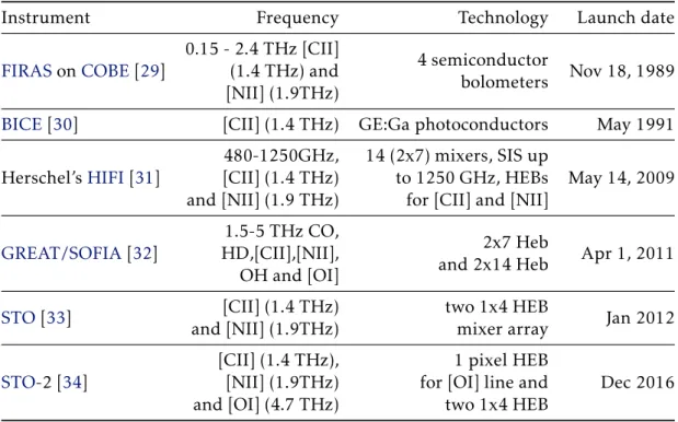
Table 1.1: State-of-the-art of GUSTO complementary missions.

Instrument Frequency Technology Launch date

FIRASonCOBE[29]

0.15 - 2.4 THz [CII] (1.4 THz) and [NII] (1.9THz)

4 semiconductor

bolometers Nov 18, 1989

BICE[30] [CII] (1.4 THz) GE:Ga photoconductors May 1991

Herschel’sHIFI[31]

480-1250GHz, [CII] (1.4 THz) and [NII] (1.9 THz)

14 (2x7) mixers, SIS up to 1250 GHz, HEBs for [CII] and [NII]

May 14, 2009

GREAT/SOFIA[32]

1.5-5 THz CO, HD,[CII],[NII], OH and [OI]

2x7 Heb

and 2x14 Heb Apr 1, 2011

STO[33] [CII] (1.4 THz) and [NII] (1.9THz)

two 1x4 HEB

mixer array Jan 2012

STO-2 [34]

[CII] (1.4 THz), [NII] (1.9THz) and [OI] (4.7 THz)

1 pixel HEB for [OI] line and two 1x4 HEB

Dec 2016

STOandStratospheric Terahertz Observatory (STO)-2 were developed by the same team asGUSTOand will serve as an effective demonstrators for the larger GUSTO focal plane unit. AlthoughGREAT/SOFIAcan observe all threeGUSTOtarget lines, it cannot devote the thousands of observing hours, since it’s an aeroplane and has a limited flight time.

(35)

C h a p t e r

2

The principle and simulation tool

2.1 Principle of a lens and antenna coupled mixer

To evaluate the coupling of the beam to an antenna lens system, the following proprieties are necessary to understand:

• Directivity [dB]; • Sidelobe level [dB];

• Full Width at Half Maximum (FWHM)or 3-dB beamwidth angle [deg]; • f# or f-number;

• Total efficiency [%] (η_total):

– Spillover efficiency [%] (η_s);

– Dielectric efficiency [%] (η_d);

– Transmission efficiency [%] (η_tr);

– Aperture efficiency [%] (η_a);

– Polarisation effi_{ciency [%] (η} p).

The directivity is a function of the angle that measure how ’directional’ an antenna’s radiation pattern is. An antenna that irradiates in all directions equally would have 1 (or 0 dB) directivity. Normally the directivity is represented by its peak value, which defines the main lobe.

The sidelobes are smaller beams that are separated from the main beam. They have undesired directions, but they can’t be eliminated. The sidelobe levels are the maximum value of the sidelobe and an acceptable level is below -15 dB.

TheFWHMis the angle range where the magnitude of the pattern goes below 50% of the main lobe peak (-3 dB). It is important for the calculation of the f#.

f# is the effective f/D ratio of the telescope being used, with f being the focal length and D the diameter of the telescope. The detector lens needs to match the one from the telescope, and to calculate it, theFWHMangle is necessary.

f# = 1 2tan(θFWHM

2 )

(2.1)

To calculate the total efficiency of the antenna/lens system, five efficiencies are mul-tiplied: the spillover effi_ciency_{, containing information about the percentage of the}

total radiated power that is actually illuminating the lens surface; the dielectric effi

-ciency,referring to losses due to conductivity of a dielectric material near the antenna;

the transmission effi_ciency_{, the total transmitted power through the lens-air interface}

divided by the total power illuminating the lens surface; theaperture effi_ciency,

describ-ing the coupldescrib-ing of the antenna to an uniform plane wave, area that would intercept the

(36)

C H A P T E R 2 . T H E P R I N C I P L E A N D S I M U L AT I O N T O O L

same power as if it was producing the wave; and thepolarisation effi_ciency, specifying

losses associated with the polarisation of the field not being align with the antenna [35].

ηtotal=ηs×ηd×ηtr×ηa×ηp (2.2)

2.2 PILRAP - Program for Integrated Lens and Reflector

Antenna Properties

The radiation pattern needed to obtain the antenna/lens proprieties refereed in the pre-vious section, was simulated with PILRAP (Program for Integrated Lens and Reflector Antenna Properties) [35]. Several parameters are necessary to start the simulation:

• Relative dielectric constant,ǫr. Ratio of the permittivity with the permittivity of vacuum, resistance when forming an electric field;

• Loss tangent. Losses associated with the electric field. On this case, it’s assumed to be always zero with silicon lens;

• Planar Feed type, type of antenna. For simulation, double slot (twin slot) was used, despite spiral antenna being used experimentally. In previous research, it was found that both spiral and twin slot result in similar beam shape;[36]

• Lens diameter [mm];

• Lens shape; Elliptical - (x/a)2_{+ (y/b)}2_{= 1, where "a" is the radius of the lens and "b"}

is the lens height not including the extension; • Extension length [mm];

• L - Length of feed. Length of the slots of the antenna; • S - Element distance. Separation of the slots;

• W - Width of element. Width of each slot.

Figure2.1shows the slot and lens dimension parameters.

Figure 2.1: Lens withHEBchip showing the dimension related parameters. The extension of the lens plus theHEBchip thickness defines the extension length used inPILRAP.

(37)

C h a p t e r

3

Results and Discussion

3.1 GUSTO optic system design

3.1.1 Proposed optic system

TheGUSTOdesign, seen in Figure3.1, was proposed to NASA in 2014.

Figure 3.1: Original GUSTO Instrument Block Diagram proposed to NASA, with 3x8 cooled HEB receivers. The colors show the organization responsible for the component.

The optical system consists of a telescope, a flip mirror for calibration, anLObox, and a cryostat with a dichroic, beamsplitter, lenses and a wiregrid inside.

Considering this is a heterodyne system, see Section 1.3, the design requires LOs signals and mixers for each frequency. TheLOs signals are located in aLObox attached to the side of the cryostat. The [NII] and [CII] beams are produced by frequency multipliers, while the [OI] is generated by aQCL. A singleQCLbeam passes through phase grating (not shown in the design) to produce the eight beams required by the [OI] array. Although the multipliers work at room temperature, theQCLrequires a 40 K cooler. The [NII]LO

and the [CII]LOsignals are merged by a wiregrid, since both [NII] and [CII]LOs have a

(38)

C H A P T E R 3 . R E S U LT S A N D D I S C U S S I O N

specific polarisation. By emitting in opposing polarisations they can be combined with minimal loss. While a dichroic filter with high transmittance for the [OI] frequency and high reflectivity for [CII] and [NII] is used to join the [OI]LOline.

The threeLOsignals travelling from theLObox enter the cryostat through a vacuum window and are combined with a focused sky beam in a 90% transmissivity and 10% reflectivity beam-splitter. Before reaching the arrays, the AS+LO beams encounter a frequency-selective surface, working as a dichroic filter, but this time, it reflects the high frequency [OI] signal to his respectiveHEBarray, while allowing the lower frequencies to pass. A wiregrid is then used to separate the [NII] and [CII] signals, since theLOsignals are polarised there will be minimal loss. On the other hand, theASphotons are linear polarised, in random directions, and at least 50% of the signal is lost in this stage. The mixer arrays consist of 8 pixels, in 4 x 2 format, strapped to the 4 K helium tank.

HEBmixer arrays down-converted signal is then filtered and amplified in a series of low-noise cryogenic microwave amplifiers.

3.1.2 Most favourable design

Since the mission selection will take place in the beginning of 2017, a new layout was designed to improve its optical efficiency for the (phase-A) study design. To do this, several goals were taken in mind:

• Increase the efficiency of theAS; • Reduce theLOsignal loss;

• Decrease the mirrors and lenses losses; • Make the alignment of the optics easier.

From several designs seen in AppendixB, the most promising one is the design shown in figure3.2.

This design uses two dichroic filters as beam-splitters and one beam-splitter. Instead of having a dichroic filter with high transmittance region and a high reflectance region, it would have a high transmittance region, but by approximating the target frequency to the critical frequency, 90% reflectance and 10% transmittance could be achieved. This way it is beam splitting the target frequency while transmitting the others. A simulated dichroic filter to show how it would work can be seen in AppendixA.

This design would achieve: • Easier to align optics; • Optics outside cryostat;

• Increase effi_{ciency of the signals.}

This way, there is no need to waste efficiency combining theLOsignals. Being outside the cryostate allows, the optical components to be aligned without opening the cryostate. On the other hand, with the components inside, with could take up to a week in Antar-tica’s weather conditions. Another advantage is the optimisation of beamsplitters and dichroics filters for each frequency.

(39)

3 . 1 . G U S T O O P T I C S YS T E M D E S I G N

Figure 3.2: New proposed design for theGUSTOballoon with outside cryostat optics and dichroic filters working as beamsplitters.

By increasing the temperature of the silicon lens, the conductivity becomes higher (more carriers), increasing the losses, so a different material may be required or a way to lower the temperature of the lens. The design of the dichroic beamsplitters, could also reveal to be a challenge. Other important problem is the increase from two cryostat window to three windows. This may increase the heat load, decreasing the maximum flight time. The heat load was calculated in Section3.1.4.

3.1.3 Optical loss calculation

Based on the optical characteristics represented in Table3.1. TheASandLOsignal losses were calculated and compared for the three frequencies for both the original design and the new design. It can be noted that all optical losses are conservative estimates.

Calculation example for the [OI] astronomical line in the original design:

100%×W3×F×FL×B6AS×D2×C×L×P (3.1)

The cryostat contains three windows due to multiple shields. For this case a 6 µm beamsplitter was used:

100%×0.83×0.91×0.80×0.75×0.982×0.87×0.5 = 12%

Only 26% of theASreaches the oxygen array. For theLOsignal, a similar equation was made. It includes the focusing on a grating that it is not represented in Figure3.1.

(40)

Table 3.1: Optical losses associated with all optic components ofGUSTO

Parameters 1.46 THz [%] 1.9 THz [%] 4.7 THz [%]

W - Window UHMW-PE [2] 80 80 80

L - LensHEB(AR coat) 10mm [37] 98 98 98

C - Coupling (Simulated) 98 97 87

F - Filter W907 84 85 91

FL - Focusing lens [2] 80 80 80

B3A - Beamsplitter forAS3 µm [38] 98 97 88 B3LO - Beamsplitter forLO3 µm [38] 98 95 83 B6AS - Beamsplitter forAS6 µm [38] 95 92 75 B6LO - Beamsplitter forLO6 µm [38] 92 87 62

D - Dichroic 98 98 98

M - Mirror 98 98 98

G - Fourier Phase Grating [2] Not used Not used 70

WG - Wire grid polariser [24] 96 96 96

P - Polarisation losses 50 50 50

A multiplier can emit a signal with 50 µW for each pixel, on the other hand, aQCLwill emit with 500 µW, but the signal will be divided by 8 after hitting the grating.

(500 µW/8)×F×FL2×G×D2×W3×B6LO×C×L×P (3.2)

The signal is reflected by the beam splitter, and not transmitted, so the signal is 100%−62% = 38%, since it’s the calculation for theLO.

(500 µW/8)×0.91×0.82×0.7×0.982×0.83×0.38×0.87×0.98×0.5 = 2.03 µW

Table 3.2 shows the results of all the optical loss calculations in the old and new design.

Table 3.2: Optical losses calculation results and their differences.

2014 design New design Difference Frequency LO signal AS signal LO signal AS signal LO signal AS signal

1.4 THz 0.59 µW 7% 0.52 µW 15% -0.07 µW +8%

1.9 THz 0.95 µW 7% 0.52 µW 16% -0.43 µW +9%

4.7 THz 2.03 µW 12% 0.278 µW 15% -1.75 µW +3%

A 6 µm beamsplitter was used for the 2014 proposed design, since, at 1.4 THz, the

LOsignal reaching theHEBis below the required 0.25 µW, with only 0.15 µW. The 6 µm beamsplitter wastes signal power for the other frequencies, like the 4.7 THz detector getting 8x theLOpower needed while losing 25% of theASsignal just with the beam-splitter. However, the new design can have a beamsplitter optimized for each frequency.

(41)

In this case, it was calculated with three dichroic/beamsplitters with 95/5 ratio of re-flectance vs transmission. Some questions may exist about the possibility of creating such beamsplitter/dichroics, they were only simulated and not tested experimentally, although calculations show some potential.

There is a big difference in the signals between the lower frequencies and higher frequencies in theAS, because the first design was designed with twin-slot antennas in mind. Since twin-slot only capture linear polarisation light, the wire grid would not make a difference. However, spiral antennas receive half the power of both polarisations, as such, a wire-grid reduces half the power.

With EachHEBrequiring 250 nW, a reversed test was also conducted. The minimum

LOpower for the system to work. Table3.3shows the results for this test.

Table 3.3:LOpower required for normalHEBoperation.

Frequency 2014 design New design 1.4 THz 21.37 µW 24.21 µW 1.9 THz 13.13 µW 24.18 µW 4.7 THz 61.59 µW 449.53 µW

The new design has less power to spare, but still far from theLOdesigned power, while doubling the AS signal at lower frequencies and increasing by 3% the 4.7 THz signal.

3.1.4 Heat load to liquid helium

To calculate the heat load to the liquid helium due to the thermal radiation through the windows, it was assumed that the window would behave like a blackbody, so the Stefan-Boltzmann’s law was used.

P A = Z Ω Z ν

Bν(ν, T)dνdΩ (3.3)

With P as the power radiated by a surface of area A through a solid angledΩin the frequency range betweenνandν+dν, at temperature T. Bν(ν, T) is the intensity of the light emitted from the blackbody surface, given by Planck’s law. It was assumed that photons from any direction would eventually heat the hellium, so the solid angle is an half-sphere.

P A =

Z

ν

B_ν(ν, T)dν

Z 2π

0 dθ

Z π₂

0 cos(φ)sin(φ)dφ

Whereθis the azimuth angle andφis the zenith angle of the half-sphere.

P=A×π

Z

ν

Bν(ν, T)dν

(42)

With windows of 10 cm of diameter (A= 79 cm2) and window temperature of 58 K the power was calculated for different ranges of frequency.

P0−4.9T Hz= 3 mW

It’s assumed that the windows will include heat filters that block any radiation above 4.9THz. However, in the second design from Figure3.2, there is a specific frequency from each LO. Hence, it is assumed that it’s also filtered in lower frequencies.

P0₋1.7T Hz= 0.4 mW P1.7₋2.1T Hz= 0.3 mW P4.5−4.9T Hz= 0.3 mW

In the default design there are two 0-4.9 THz windows, meaning a 6 mW loss. The second design despite having one more window, since they are frequency specific, the heat load to the helium is only 1 mW. These calculations don’t take into account that there are multiple shields, and take into account that every photon will reach the helium. Hence, the real values, will be lower. Since the heat load to the helium is 22 mW, from calculations in the proposal, the windows don’t represent a meaningful source of loss.

3.1.5 Most favourable design 2

Professor Christopher Walker from the University of Arizona, principal investigator and responsible for the optics of theGUSTOproject, has updated the design forGUSTO. The new design can be seen in Figure3.3.

Several similar conclusions were made: • Optics outside cryostat;

• Beam splitter optimised for the frequency; • Increase number of cryostat windows to three.

Also, new restrictions were introduced, like the telescope must be in the same axis as the detectors. The design also combines 1.4 THz and 1.9 THz lines, since they are very similar frequencies, the optical components losses are also very similar, and it’s not necessary a trade-offbetween theLOandASsignal power. Another distinction, is the integration of theQCLin the cryostat, helping it keep the 40 K temperature.

With this new design, instead of having two 4x2 arrays, one for the [NII] and other for [CII], there is a detector box with 4x4 array, where half will detect one frequency and the other half the other frequency, removing the need to separate both frequencies. TheAS

will be direct for the [NII] and [CII] detectors, while the [OI] is separated with a dichroic. Again, the design was studied to find any problems and to improve its efficiency. From several designs seen in AppendixC.1, the most promising one is shown in Figure3.4.

(43)

Figure 3.3: Christopher Walker’s new design, with outside optics and theQCLinside the cryostat. AQCLfrequency lock loop is introduced to stabilise theQCLfrequency.

Figure 3.4: Most favourable design, with telescope beam directly to [OI] channel detectors and with less optical components.

(44)

This design, instead of having theASdirectly to the [CII] and [NII] lines, it is direct to the [OI] line. It will keep the same efficiency for the two lower frequencies, but it will bring some improvement for the [OI] line:

• One or two less optical components; • Small improvement in efficiency.

The beam splitter used, can have a dichroic on top of it, reflecting the [OI] line, or it can use one of the simulated dichroic/beam splitters, from Appendix A, reducing one more component.

3.1.6 Optical loss calculations 2

The optical losses of each design were again compared:

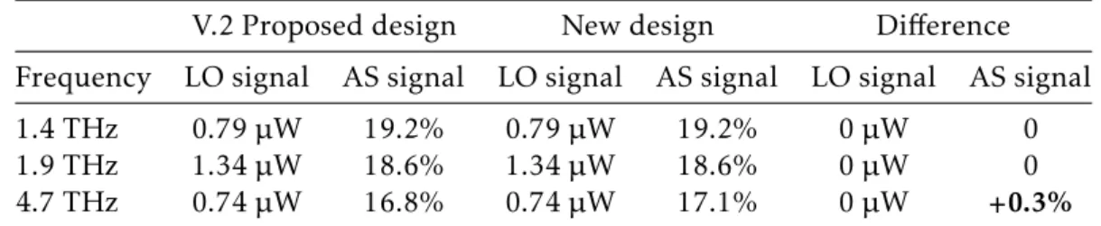
Table 3.4: Optical losses calculation results for the two new designs and their diff_erences.

V.2 Proposed design New design Difference Frequency LO signal AS signal LO signal AS signal LO signal AS signal

1.4 THz 0.79 µW 19.2% 0.79 µW 19.2% 0 µW 0

1.9 THz 1.34 µW 18.6% 1.34 µW 18.6% 0 µW 0

4.7 THz 0.74 µW 16.8% 0.74 µW 17.1% 0 µW +0.3%

The new design has minimal optical impact, only improving by +0.3% on the [OI]. Since the [OI] is the least measured line by the scientific community, it is the most im-portant frequency. For that reason, ASis directly pointed to the [OI] detectors, which should help improve the signal. It’s also important to notice the reduction of the optical components by two, helping the alignment.

The reversed study was also repeated:

Table 3.5:LOpower required for the two new designs for normalHEBoperation. Both designs have the sameLOsignal.

Frequency V.2 Proposed design and New design

1.4 THz 15.75 µW

1.9 THz 9.29 µW

4.7 THz 84.28 µW

Both the new design and the proposed have the sameLOpower. The [NII] line is the only one with less power to spare.

(45)

3 . 2 . L E N S D E S I G N

3.2 Lens design

3.2.1 Beam shape of a lens-antenna with a 5 mm diameter lens

The 10 mm lens, experimentally, shows the best results in terms ofNoise temperature, but for theGUSTO, it has a f# too large. Previously simulations show that the 10 mm has a f#136 at 4.7 THz, while it’s necessary to match a f#19.6 telescope.

The 3.1 mm lens can lower the f# to f#41, but theNoise temperature, experimentally, increases. To achieve f#19.6, it is necessary to choose a diameter of 1.5 mm, which is not realistic for a practical mixer. To solve this problem, additionally optics will be necessary between the telescope and the mixer to match the beams. However, the difference for the 10 mm lens is substantial, so a 5 mm one was tested. It is expected to have betterNoise temperaturethan the 3.1 mm lens and a better f# than the 10 mm lens, we will have the best of two worlds. Parameters used for the simulation can be seen in Table3.6.

Table 3.6: Parameters used for the 5 mm lens simulation.

Parameters 1.4 THz 1.9 THz 4.7 THz

Dielectric constant 11.4 11.4 11.4

Loss tangent 0 0 0

Diameter 5 mm 5 mm 5 mm

Shape of lens Elliptical Elliptical Elliptical Planar Feed Type Double Slot Double Slot Double Slot

L - Length of feed 0.2847 0.3 0.3

S - Element distance 0.1633 0.17 0.17

W - Width of Element 5% 5% 5%

Table3.7and Figure3.5show the results from the simulation.

Table 3.7: Simulation results of the 5 mm lens.

Parameters 1.4 THz 1.9 THz 4.7 THz

3-dB beamwidth 2.8 2.0 0.8

10-dB beamwidth 4.6 3.5 1.4

Sidelobe level -20.0 dB -20.3 dB -20.3 Directivity 34.9 dBi 37.4 dBi 45.2 Total efficiency 60.0% 55.4% 56.2%

f# 21 28 68

At 1.4 THz and 1.9 THz, with f#21 and f#28 respectively, the f# isn’t very different from the target f#19.6, however, 4.7 THz has a f#68.

Decreasing the lens dimensions, decreases the f#, but since there is a limit, maybe other parameters will affect the f#. All the antenna parameters can’t be changed due to matching impedance between the antenna and the HEB, and the relative dielectric constant is a constant of the material. So the lens shape and extension length are the only ones that may affect it.

(46)

Figure 3.5: Power beam pattern of 5 mm lens and antennas at 1.4 THz, 1.9 THz and 4.7THz.

3.2.2 Optimising the f# by changing the lens shape and extension length

The lens shape ellipticity is defined by the ratio of "b" by "a", seen in Section2.1. Small changes in the extension length and in the ellipticity have huge effects in efficiency and the f#, so the extension length ranges only from 0.7 to 0.82 with a 0.02 step and the ellipticity ranges from 1.03 to 1.08 with a step of 0.005.

Table 3.8: Simulation parameters for the optimisation of the f#.

Parameters Value Parameters Value

Frequency 4.7 THz Planar feed type Double slot

Loss tangent 0 Length of feed 0.3

Dielectric constant 11.4 Element distance 0.17

Diameter 5 mm Width of element 5%

Extension length 0.7-0.82 µm Ellipticity 1.03-1.08

The matching patterns between the two plots infers that to achieve f#10 there will be a major loss of efficiency. To further confirm the relation between efficiency and the f#, the plot of the Figure3.7shows the f# as a function of the efficiency.

The results show that to lower the f#, the effi_{ciency has drop by 25%. This outcome} proves that it isn’t reliable to change the extension or the lens dielectric constant, and it will be necessary additional optics to match the f# numbers.

(47)

3 . 2 . L E N S D E S I G N

Figure 3.6: Contour of the effi_{ciency and the optical f# of a lens-antenna systemas a} function of the lens extension length and ellipticity.

Figure 3.7: Optical f# of the lens-antenna as a function of the efficiency

(48)

3.2.3 Beam’s response to changing extension length and dielectric constant of the lens

A lens with 10 mm and three lenses with 3.1 mm, each designed for a different relative dielectric constant (11.7 - L1, 11.4 - L2 and 11.2 - L3), had theNoise temperaturetested with spiralHEBs in the work of the master thesis student José Rui Silva [39]. The results can be seen in Figure3.8.

Figure 3.8: Receiver noise temperature measurement in the vacuum setup for one 10 mm diameter lens and three 3.1 mm diameter lenses. L1 was measured with a ticker beamsplitter (BS), so based on the results of of L2 and L3, L1 was corrected to allow comparisons. [39]

Lens 3 shows an increase of 14% in Noise temperature, while lenses 1 and 2 are considered equal due to errors associated with the experimental setup. However, the 10 mm lens shows a 32% decrease in noise temperature in relation to lenses 2 and 1. This is not expected since, based on simulation, the effi_{ciency on both lenses should be similar.} One way to explain is that it is due to the measuring method, as there are two methods: with a blackbody inside the cryostat (vacuum setup) and with a blackbody outside (air setup). The blackbody in the vacuum setup is smaller in size, so there may be a problem in centralising the radiation on the 3.1 mm lens. The air setup, on the other hand, has a blackbody that cover the entire area. To test this theory lens 1 and the 10 mm lens were tested in the air setup. The results can be seen in Figure3.9.

The air setup is expected to have increased noise, due to the effective noise introduced by the air and the cryostat window losses. However, the difference in noise reduces to

(49)

3 . 2 . L E N S D E S I G N

Figure 3.9: Comparison between noise temperature measurements in air setup vs vacuum setup in both 10 mm diameter lens and one 3.1 mm lens (L1) [39].

16% in the air setup. Part of the problem was solved, but it still doesn’t fully explain the results. It was speculated that the extension length of the lens could be wrongly measured or the relative dielectric constant to be different than expected, considering that it’s hard to measure at 4 K. To prove this hypothesis, the influence of the dielectric constant and the extension length of the antenna on the efficiency of the antenna-lens system, was simulated.

Table 3.9: Values used for each parameter in the simulation programPILRAP.

Parameters Value Parameters Value

Frequency 2.5 THz Planar feed type Double slot Design frequency 2.5 THz Length of feed 0.3 Diameter 3.1 mm Element distance 0.17 Loss tangent 0 Width of element 5%

The results of this simulation can be seen in Figure3.10. Throughout the dielectric values and throughout the extension length values, the efficiency drop is similar. So for further analysis, the efficiency drop was plotted for the expected_ǫ_r of 11.4, Figure3.11, and for the 0.474 mm and 0.514 mm, Figure3.12. The 3.1 mm lens was designed with an extension length of 0.474 mm, but a 0.04 mm offset was found to improve coupling experimentally.

(50)

Figure 3.10: Total lens efficiency as a function of the extension length and the relative dielectric constant.

Figure 3.11: Efficiency as a function of extension length, assuming a relative dielectric constant of 11.4.

(51)

3 . 2 . L E N S D E S I G N

Figure 3.12: Efficiency as a function of the dielectric constant for 0.514 mm extension length and 0.482 mm.

A 0.514 mm extension would mean a low efficiency of 34.9% at a_ǫ_rof 11.4. The lens with 0.474 mm was optimised for aǫ_rof 11.7, but even at 11.4, the effi_{ciency is still high,} 54.9%. This further proves that the measured extension length may be wrongly mea-sured. Analysing Figure3.11, and assuming that the value 11.4 is correct, the measured extension length, 0.514 mm, may be wrong for at least 28 µm.

The 10mm lens used has an extension of 1.569 mm, which gives an efficiency of 52.9%. Assuming that the 3.1mm lens has an efficiency of 34.9%, it means that the extension length was measured right, and there is a 34% relative drop in efficiency. This 34% is similar to noise temperature difference at vacuum, but it would not explain the air setup difference.

The difference between air setup noise temperature measurements is 16% and the vacuum setup noise temperature is 32%. In the vacuum setup, the radiation may not be centralised in the lens, while in the air setup, covers the entire area so the 3.1 mm lens is covered. Meaning that the 16% should be a problem with the lens optimisation.

This difference, assuming a 11.4 dielectric constant is correct, and knowing that at 0.492 mm extension length, the effi_{ciency is 52.9% (the same as the 10 mm lens), a 16%} loss in efficiency occurs at an extension length of 0.503 mm. This corresponds to a 11 µm difference to achieve the same optimisation state.

(52)

3.2.4 Measurement of lens dimensions to explain noise temperature results

To prove that the lens may have the wrong dimensions, it was measured with two different methods, with an optical microscope connected to a micrometre, so the dimension is based on the difference in focus, and with a MitutoyoCoordinate Measuring Machine (CMM) Crysta-Apex C. TheCMMand a zoom in of the lens can be seen in Figure3.13.

As seen in Section2.1, the lens shape is characterised by the lens height without the extension (b), half the lens diameter (a), and the extension length, but since the lens height goes inside the extension, it’s impossible to measure both the "b" value and the extension, so only the total lens height is measured.

(a) (b)

Figure 3.13: a) CMM used to measure the lens dimensions. b) 3.1 mm lens strapped between two clamps.

The design dimensions for each lens can be seen in Table 3.10, which shows the measurements of the lens height. Since, the dielectric constant of silicon at 4 K was not known accurately, three 3.1 mm lens were optimised for three different dielectric constants, 11.7, 11.4 and 11.2.

Every optical measurement portrayed is the average of 10 measures, by defocusing and refocusing. On the other hand, theCMMis the average of 3 measures due to the time it takes per measure. The variation between the 10 optical measures was±2 µm, while

the variation in theCMM, even though the resolution is about 0.1 µm, was±5 µm. These

results can be explained by the measurement method. While the optical measurement is a non-contact method, theCMM, being a contact method, may be susceptible to any dust or particle in the lens or in the surface, despite the surfaces being cleaned with a nitrogen gas blow.

Hence the optical measurement is precise, but it may have an offset, consequently, being not very accurate. However, since it only matters the relative difference between

(53)

3 . 2 . L E N S D E S I G N

the lenses to explain the noise differences, the optical measurement is used for conclusion purposes.

Table 3.10: Results of the lens height measurements compared to the expected design dimensions.

Lens Expected

height [mm]

Optical measure [mm]

Difference [µm]

CMM mea-sure [mm]

Difference [µm]

10 mm 6.457 6.460 +3 6.465 +8

3.1 mm lens 1 1.755 1.773 +18 1.766 +11

3.1 mm lens 2 1.764 1.771 +7 1.764 +0

3.1 mm lens 3 1.769 1.780 +11 1.776 +7

To calculate the extension length, we measured the entire lens height including the extension length and subtracted the "b" expected value. The "b" value is assumed to be correct, considering the lens shape was measured previously and it had an error in the range of nanometres.

Table 3.11: Extension length without the substrate thickness for the optical measurement. It also shows the distance from optimum extension, simulated inPILRAP.

Lens _{extension [mm]}Expected _{measure [mm]}Optical Variation_[µm] _{extension [µm]}∆optimum

10 mm 1.229 1.232 +3 +27

3.1 mm lens 1 0.134 0.152 +18 +23

3.1 mm lens 2 0.141 0.148 +7 +22

3.1 mm lens 3 0.145 0.156 +11 +32

This extension does not include the substrate thickness of the detector, which will be glued to the lens. This way, the total extension will be the substrate thickness plus the values of extension obtained in the previous calculation. All noise measurements were done with the same detector chip, i.e. the same substrate. The substrate thickness is designed to have 340 µm, but both the optical and theCMMmeasured 350 µm.

The three 3.1 mm lens and the 10 mm lens were simulated for±50 µm from the ideal

extension with maximum efficiency, seen in Figure3.14. This way we can compare real dimensions, including a substrate thickness of 350 µm versus the ideal.

The simulation shows that the decreasing ratio is similar no matter the lens dimen-sions. By decreasing the lens diameter, the focal length decreases by the same ratio, so the angle of incidence in the detector is the same. With the same angle, the same antenna size, and being the same chip, the decrease in efficiency is the same.

Even though the 3.1 mm lens 1 was supposed to have a smaller extension than lens 2, the length is bigger than expected, making them very similar. Explaining the similar noise temperature results seen in the Figure3.8. Like lens 1, lens 3 extension also increased in relation with lens 2, increasing the difference in efficiencies. This also reflects in the noise

(54)

Figure 3.14: Efficiency as a function of the variation from the optimum extension length for each lens. Marked in circles is the diff_{erence between the optimum extension and the} optical extension measured for the four lens.

temperature value, lens 3, with just 10 µm in difference in extension, has an increase of 14% in noise temperature.

Data explains the diff_{erence in the 3.1 mm lens, but it doesn’t explain for the 10 mm.} The simulations show similar efficiency, when the noise difference in the vacuum setup is 32% and 16% in the air setup.

3.2.5 Optimum extension length of the lens with changing relative dielectric constant

To explain the difference between the 10 mm lens and the 3.1 mm lenses, the optimum extension needs to change more in the 10 mm than in the 3.1 mm. This was tested by changing the lens shape, the frequency and the antenna shape, but with no success. However, changing the relative dielectric constant has a bigger impact in the 10 mm lens than in the 3.1 mm. A plot of the efficiency of the four lenses as a function of the relative dielectric can be seen in Figure3.15. The lens dimensions used for the simulation where based on the optical measurements from Section3.2.4.

Lens 1 and Lens 3 have a 23% noise difference, and lens 1 and the 10 mm lens have a 26% difference in the vacuum setup, as seen in Figure3.8, and at a relative dielectric of 11.2, they have a diff_{erence of e}ffi_{ciency of 6.4% and 5.5%, respectively. This could} explain the difference in the receiver noise temperature between the 10 mm lens and the 3.1 mm lenses.

(55)

3 . 2 . L E N S D E S I G N

Figure 3.15: Efficiency as a function of the relative dielectric constant, using the simula-tion results with the optical measured dimensions of the lenses.

It’s very difficult to measure the dielectric constant of silicon at 4 K, that’s the whole reason why three 3.1 mm lenses were made, one for each dielectric constant, to try to find the one with best results. Having that in consideration, the literature value is 11.4 [40]. There are too many factors that could cause errors related with the measure of the noise temperature and lens dimensions. Also, there isn’t enough repetition, to claim that the relative dielectric is 11.2. Nonetheless, it opens interesting issue and asks for further experimental verification.

(56)

(57)

C h a p t e r

4

Conclusions and future perspectives

This thesis optimises the optical system of the balloon GUSTO and explores lens design characteristics of the detection.

For the optical design a new concept was introduced, a cryostat with windows for each frequency. This allows the placement of optical components outside the cryostat, for easy alignment, making unnecessary to mergeLOsignals, thus reducing losses. Since the cryostat reaches a temperature of 4 K, due to thermal radiation through the windows, this could increase the heat load. However, it was calculated that as a results of the windows being more frequency specific, filters can block most of the radiation and actually de-crease the heat load. WithLObeams separated, the beamsplitters can also be optimised for each frequency, and by using a new approach, with dichroic filters as beamsplitters, the number of optical components can be reduced even further. By reducing the optical components, an increase in optical signal was achieved. This concept was presented to a group of astronomers that found the frequency specific windows concept innovative. Hence, the concept is a candidate design for GUSTO and it may be applied for future space missions.

Professor Christopher Walker principal investigator of the GUSTO project, updated the optical design, reaching similar conclusions. His design also placed the optics outside the cryostat, increased the cryostat windows to three and allowed beamsplitters specific for the frequency. The main differences are the QCLbeing placed inside the cryostat, helping it to refrigerate, and combining the [NII] and [CII] pixels. [NII] and [CII] have similar frequencies, so the beamsplitter and the window can still be optimised without having losses separating both astronomical lines. The design was again optimised, in-creasing slightly the [OI] astronomical line, while potentially reducing the number of optical components by two.

One of the main challenges of the GUSTO optical system is the coupling of the tele-scope beam to an antenna lens system. A 10 mm diameter lens offers a good sensitivity of the detection (low noise temperature), however, the f# number is too large comparing with the f# number of the telescope, f#136 compared to f#19.6 respectively. On the other hand, a 3.1 mm diameter lens shows a better coupling (similar f# number), but the noise temperature increases. A 5 mm diameter lens was then simulated, showing results that have the best of the two worlds. At 1.46 THz and 1.9 THz the f# number was similar to the telescope, demonstrating the feasibility to use smaller lens for GUSTO’s heterodyne arrays at these frequencies. However at 4.7 THz the f# number was still too big. To solve this, it was simulated lenses with diff_{erent ellipticities and extension length, concluding} that reducing f# is impossible and that additional optics will be necessary to match the telescope with the receivers.