HESSD
11, 10787–10828, 2014How over 100 years of climate variability may affect estimates
of potential evaporation
R. P. Bartholomeus et al.
Title Page
Abstract Introduction
Conclusions References
Tables Figures
◭ ◮
◭ ◮
Back Close
Full Screen / Esc
Printer-friendly Version Interactive Discussion
Discussion
P
a
per
|
Discus
sion
P
a
per
|
Discussion
P
a
per
|
Discussion
P
a
per
|
Hydrol. Earth Syst. Sci. Discuss., 11, 10787–10828, 2014 www.hydrol-earth-syst-sci-discuss.net/11/10787/2014/ doi:10.5194/hessd-11-10787-2014
© Author(s) 2014. CC Attribution 3.0 License.
This discussion paper is/has been under review for the journal Hydrology and Earth System Sciences (HESS). Please refer to the corresponding final paper in HESS if available.
How over 100 years of climate variability
may a
ff
ect estimates of potential
evaporation
R. P. Bartholomeus1, J. H. Stagge2, L. M. Tallaksen2, and J. P. M. Witte1,3
1
KWR Watercycle Research Institute, P.O. Box 1072, 3430 BB Nieuwegein, the Netherlands
2
Department of Geosciences, University of Oslo, P.O. Box 1047, Blindern, 0316 Oslo, Norway
3
VU University, Institute of Ecological Science, Department of Systems Ecology, de Boelelaan 1085, 1081 HV Amsterdam, the Netherlands
Received: 28 July 2014 – Accepted: 28 August 2014 – Published: 24 September 2014
Correspondence to: R. P. Bartholomeus ([email protected])
HESSD
11, 10787–10828, 2014How over 100 years of climate variability may affect estimates
of potential evaporation
R. P. Bartholomeus et al.
Title Page
Abstract Introduction
Conclusions References
Tables Figures
◭ ◮
◭ ◮
Back Close
Full Screen / Esc
Printer-friendly Version Interactive Discussion
Discussion
P
a
per
|
Discus
sion
P
a
per
|
Discussion
P
a
per
|
Discussion
P
a
per
|
Abstract
Hydrological modeling frameworks require an accurate representation of evaporation fluxes for appropriate quantification of e.g. the soil moisture budget, droughts, recharge and groundwater processes. Many frameworks have used the concept of potential evaporation, often estimated for different vegetation classes by multiplying
5
the evaporation from a reference surface (“reference evaporation”) with crop specific scaling factors (“crop factors”). Though this two-step potential evaporation approach undoubtedly has practical advantages, the empirical nature of both reference evaporation methods and crop factors limits its usability in extrapolations and non-stationary climatic conditions. In this paper we assess the sensitivity of potential
10
evaporation estimates for different vegetation classes using the two-step approach when calibrated using a non-stationary climate. We used the past century’s time series of observed climate, containing non-stationary signals of multi-decadal atmospheric oscillations, global warming, and global dimming/brightening, to evaluate the sensitivity of potential evaporation estimates to the choice and length of the calibration period.
15
We show that using empirical coefficients outside their calibration range may lead to systematic differences between process-based and empirical reference evaporation methods, and systematic errors in estimated potential evaporation components. Such extrapolations of time-variant model parameters are not only relevant for the calculation of potential evaporation, but also for hydrological modeling in general, and they may
20
limit the temporal robustness of hydrological models.
1 Introduction
Evaporation from the vegetated surface is the largest loss term in many, if not the most, water balance studies on earth. As a consequence, an accurate representation of evaporation fluxes is required for appropriate quantification of surface runoff, the soil
25
moisture budget, transpiration, recharge and groundwater processes (Savenije, 2004).
HESSD
11, 10787–10828, 2014How over 100 years of climate variability may affect estimates
of potential evaporation
R. P. Bartholomeus et al.
Title Page
Abstract Introduction
Conclusions References
Tables Figures
◭ ◮
◭ ◮
Back Close
Full Screen / Esc
Printer-friendly Version Interactive Discussion
Discussion
P
a
per
|
Discus
sion
P
a
per
|
Discussion
P
a
per
|
Discussion
P
a
per
|
However, despite being a key component of the water balance, evaporation figures are usually associated with large uncertainties, as this term is difficult to measure (Allen et al., 2011) or estimate by modeling (Wallace, 1995).
Research attempting to model the evaporation process has a long history (Shuttleworth, 2007). This research took two parallel tracks, with the meteorological
5
community developing process-based models of surface energy exchange and the hydrological community considering evaporation as a loss term in the catchment water balance (Shuttleworth, 2007). To quantify the evaporation loss term, many hydrological modeling frameworks have used the concept of potential evaporation (Federer et al., 1996; Kay et al., 2013; Zhou et al., 2006), defined as the maximum rate of evaporation
10
from a natural surface where water is not a limiting factor (Shuttleworth, 2007). With the progression from catchment-scale lumped models (such as HBV, Bergström and Forsman, 1973) to distributed models with increasing spatial resolution and spatially resolved data (such as SHE, Abbott et al., 1986), the explicit representation of land surface water budgets also increased (Ehret et al., 2014; Federer et al., 1996).
15
To this end, estimation of evaporation from a variety of land surfaces within the simulated domain is needed (Federer et al., 1996). More models were developed that included vegetation explicitly, commonly by describing the stomatal conductance of the vegetation as a function of environmental drivers (see Shuttleworth, 2007, and references therein). However, until now these models are rarely used in practice and
20
merely have a scientific meaning.
Parallel to this development, the irrigation engineering community refined the traditional potential evaporation approach (Shuttleworth, 2007). They developed the “two-step approach” (Doorenbos and Pruitt, 1977; Penman, 1948; Zhou et al., 2006; Feddes and Lenselink, 1994; Vázquez and Feyen, 2003; Hupet and Vanclooster, 2001),
25
HESSD
11, 10787–10828, 2014How over 100 years of climate variability may affect estimates
of potential evaporation
R. P. Bartholomeus et al.
Title Page
Abstract Introduction
Conclusions References
Tables Figures
◭ ◮
◭ ◮
Back Close
Full Screen / Esc
Printer-friendly Version Interactive Discussion
Discussion
P
a
per
|
Discus
sion
P
a
per
|
Discussion
P
a
per
|
Discussion
P
a
per
|
approach has even expanded outside the field of irrigation engineering into hydrological modeling frameworks. Crop factors are now being applied in 1-D hydrological models (e.g. Tiktak and Bouten, 1994), spatially lumped models (e.g. Driessen et al., 2010; Calder, 2003), and spatially distributed hydrological models (e.g. Ward et al., 2008; Shabalova et al., 2003; Trambauer et al., 2014; Van Roosmalen et al., 2009; Lenderink
5
et al., 2007; Bradford et al., 1999; Guerschman et al., 2009; Sperna Weiland et al., 2012; Van Walsum and Supit, 2012; Vázquez and Feyen, 2003).
With the development of the two-step potential evaporation approach, different equations to simulate reference evaporation have been suggested (Federer et al., 1996; Bormann, 2011; Shuttleworth, 2007) for use in both regional and global
10
hydrological models (e.g. Sperna Weiland et al., 2012; Haddeland et al., 2011). However, due to their empirical nature, these equations are limited in their transferability in both time and space (Feddes and Lenselink, 1994; Wallace, 1995). Since the increasing need for predictions under global change (land use and climate) (Ehret et al., 2014; Coron et al., 2014; Montanari et al., 2013), the empirical nature of most
15
commonly used potential evaporation approaches is a serious drawback (Hurkmans et al., 2009; Wallace, 1995; Shuttleworth, 2007; Witte et al., 2012). Thus, although the two-step approach may be warranted for practical reasons, both the reference evaporation and estimated crop factors include a series of empirical parameters that may affect the validity and general applicability of the estimated potential evaporation
20
for a specific vegetation class.
Since the term “potential evaporation” has been used by the hydrologic community to refer to several different combinations of evaporation components in the past, it is important to re-introduce these definitions and to be very specific about nomenclature in future evaporation research. Total evaporation (Etot) from a vegetated surface is
25
the sum of three fluxes: transpiration (Et), soil evaporation (Es) and evaporation of
intercepted water (Ei).Et andEsoccur at a potential rate when the availability of water (soil moisture or interception) is not limiting. As we will only focus on potential rates in this paper, all values should be interpreted as potential, unless stated otherwise.
HESSD
11, 10787–10828, 2014How over 100 years of climate variability may affect estimates
of potential evaporation
R. P. Bartholomeus et al.
Title Page
Abstract Introduction
Conclusions References
Tables Figures
◭ ◮
◭ ◮
Back Close
Full Screen / Esc
Printer-friendly Version Interactive Discussion
Discussion
P
a
per
|
Discus
sion
P
a
per
|
Discussion
P
a
per
|
Discussion
P
a
per
|
Reference evaporation (Eref) is defined as the rate of evaporation from an extensive
surface of green grass, with a uniform height of 0.12 m, a surface resistance of 70 s m−1,
an albedo of 0.23, actively growing, completely shading the ground and with adequate water (Allen et al., 1998). By definition, Ei is not part of reference evaporation, as
it is defined for a plant surface which is externally dry (Federer et al., 1996; Allen
5
et al., 1998). Often, the term reference evapotranspiration is used instead, which is the sum of transpiration (Et) and soil evaporation (Es). By definition (Allen et al., 1998)
the reference crop completely shades the ground and henceEs will be zero andEref equalsEtof the reference crop (at least for daily estimates, when the soil heat flux can be assumed zero). This is in agreement with the definition of Penman (1956) who also
10
stated that the often-used expansion of the term “reference evaporation” to “reference evapotranspiration” was unnecessary.
Eref is used in the two-step method to estimate the potential evaporation, Ep, of a crop or vegetation stand. Ep will reduce to the actual evaporation, Ea, in case of water shortage or waterlogging. Here, we focus on the estimation of Ep from Eref, by
15
multiplyingErefwith a crop factorK (Allen et al., 2005, 1998; Feddes, 1987; Penman, 1956). Different applications of crop factors exist:
– Kt corrects for potential transpiration of a crop with a dry canopy only, i.e. Et=
Kt·Eref. This corresponds to the basal crop factors defined by Allen (2000), which
are equivalent to the approach of Penman (1956).
20
– Ktscorrects for both potential transpiration and potential soil evaporation for a crop with a dry canopy, i.e.Et+Es=Kts·Eref. This corresponds to the single crop factors
defined by Allen et al. (1998).
– Ktotcorrects for potential total evaporation, i.e. transpiration, soil evaporation, and interception. UsingKtotwithErefdirectly givesEtot, i.e.Etot=Ktot·Eref.
25
HESSD
11, 10787–10828, 2014How over 100 years of climate variability may affect estimates
of potential evaporation
R. P. Bartholomeus et al.
Title Page
Abstract Introduction
Conclusions References
Tables Figures
◭ ◮
◭ ◮
Back Close
Full Screen / Esc
Printer-friendly Version Interactive Discussion
Discussion
P
a
per
|
Discus
sion
P
a
per
|
Discussion
P
a
per
|
Discussion
P
a
per
|
quantities that soil water is not limiting for plant growth (Feddes, 1987). Sprinkling, however, leads to interception. So, crop factors like those of Feddes (1987) implicitly involveEi. Therefore Feddes (1987) emphasizes that the presented crop factors “are averages taken over a population of “average”, “dry”, and “wet” years, that will certainly not be homogeneously distributed”. The crop factor approach by Feddes (1987) is
5
different from the single crop factor approach of Allen et al. (1998), as crop factors from the latter are by definition applied to correct forEt+Es, or forEtonly (Allen, 2000). However, Allen et al. (1998) indicate that their crop factors should be multiplied with a factor 1.1–1.3 if interception, due to sprinkling irrigation for example, is involved. This indicates thatEi could significantly affect potential evaporation from a vegetated
10
surface. AsEiis largely driven by precipitation, a term that is generally not incorporated inEref methods, it has already been stated that the crop factor approach only makes sense in times of drought, when interception does not contribute to the total evaporation (De Bruin and Lablans, 1998). This condition is especially relevant for tall forests, which intercept a higher percentage of rain water, under climatological conditions
15
with significant rainfall (De Bruin and Lablans, 1998). Nevertheless, this crop factor approach is used in practice (Van Roosmalen et al., 2009).
The objective of this paper is to assess the sensitivity of potential evaporation estimates for different vegetation classes using the commonly used two-step approach when calibrated based on a non-stationary climate. To this end, we use century long
20
meteorological observations representing the historic variability in climatic conditions at the De Bilt, the Netherlands climate monitoring station. The past century’s global warming, dimming and brightening periods (Suo et al., 2013; Stanhill, 2007; Wild, 2009; Wild et al., 2005), and their effects on evaporation provide an opportunity to evaluate the robustness of the two-step estimation of potential evaporation for non-stationary
25
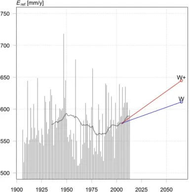
conditions. Given the 20th century climate induced variability inErefand the projected
no-analogue ongoing increase for the near future (Fig. 1), it is of great importance to recognize the limitations of applying empirical coefficients outside their calibration
HESSD
11, 10787–10828, 2014How over 100 years of climate variability may affect estimates
of potential evaporation
R. P. Bartholomeus et al.
Title Page
Abstract Introduction
Conclusions References
Tables Figures
◭ ◮
◭ ◮
Back Close
Full Screen / Esc
Printer-friendly Version Interactive Discussion
Discussion
P
a
per
|
Discus
sion
P
a
per
|
Discussion
P
a
per
|
Discussion
P
a
per
|
range (i.e. extrapolation). This applies not only to transferring coefficients in space, as between climatic regions (Allen et al., 1998), but also in time.
The 20th century global surface temperature can be characterized by two major warming periods; the first one from about 1925–1945, followed by a period of cooling, and a second starting in about 1975 and continuing to the present (Jones and Moberg,
5
2003; Yamanouchi, 2011). While the variations in temperature until the 1970s can be related to changes in global radiation, i.e. global dimming and brightening, this relationship no longer holds for the rapid warming since 1975 (Wang and Dickinson, 2013). Empirical equations for reference evaporation that use either radiation or temperature implicitly assume a relationship between the two variables. Given the
10
nonlinearity of evaporation components, it is not only questionable whether empirical equations for reference evaporation will be applicable under future climatic conditions (Shaw and Riha, 2011), but also whether they are applicable for the recent past.
In this study we systematically unravel the use of the two-step approach to simulate potential evaporation and identify systematic errors that may be introduced when
15
empirical coefficients are applied outside their calibration period. Such extrapolations of time-variant model parameters are not only relevant for the calculation of potential evaporation, but also for hydrological modeling in general, thus limiting the temporal robustness of hydrological models (Ehret et al., 2014; Karlsson et al., 2014; Coron et al., 2014; Seibert, 2003).
20
2 Methods
2.1 General approach
We use 108 years of meteorological observations to quantify the sensitivity of potential evaporation when calibrated using a non-stationary climate for various natural vegetation classes using the two-step approach. We investigate how empirical
25
HESSD
11, 10787–10828, 2014How over 100 years of climate variability may affect estimates
of potential evaporation
R. P. Bartholomeus et al.
Title Page
Abstract Introduction
Conclusions References
Tables Figures
◭ ◮
◭ ◮
Back Close
Full Screen / Esc
Printer-friendly Version Interactive Discussion
Discussion
P
a
per
|
Discus
sion
P
a
per
|
Discussion
P
a
per
|
Discussion
P
a
per
|
evaporation for different vegetation classes, by applying empirical coefficients outside their calibration period. We vary the calibration period in both length (2–30 years) and reference period (in 1906–2013).
First (Sect. 2.3), we simulate reference evaporation according to the process-based Penman–Monteith equation (Eref_PM), which is considered the international standard
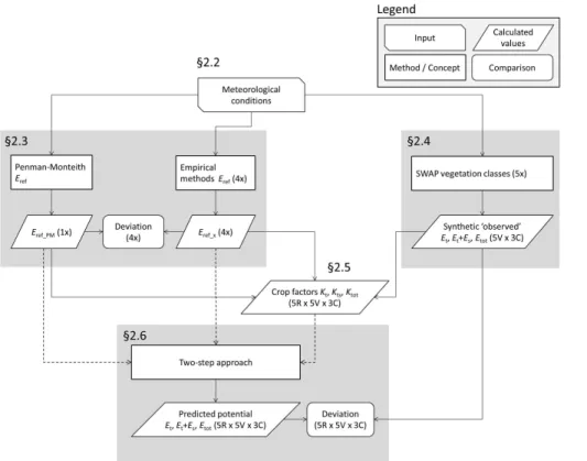
5
method for estimating reference evaporation (Allen et al., 1998). In addition, we apply four empirical equations that contain constants derived for a calibration period (Fig. 2: §2.3). From these simulations, we identify deviations between each empirical Eref method and theEref_PM(Fig. 2: §2.3).
Secondly (Sect. 2.4), we generate time series of the main components of potential
10
evaporation, i.e. synthetic series ofEt,Es and Ei, for five different vegetation classes, using the Soil–Vegetation–Atmosphere Transfer (SVAT) scheme SWAP (Kroes et al., 2009; Van Dam et al., 2008) (Fig. 2: §2.4). SWAP allows users to simulate potential evaporation for different vegetation classes directly (i.e. one-step approach), by parameterizing the Penman–Monteith equation for each vegetation class implicitly
15
rather than using crop factors. These synthetic series are considered “observations” throughout the paper for all comparisons with estimates from the two-step approach.
Finally (Sect. 2.5), we derive monthly crop factors for each vegetation type (5×) and for eachErefmethod (5×) based on the synthetic data ofEt,EsandEifor a calibration
period (e.g. 1906–1935) to simulate crop factor estimation using field measurements
20
(Fig. 2: §2.5). We use different (3×) definitions of crop factors: for transpiration (Kt), for transpiration plus soil evaporation (Kts) and for total evaporation (Ktot). Next, we apply the two-step approach, usingErefand crop factors from the calibration period to
calculate daily “predicted” evaporation components (3×) for each vegetation class (5×) and eachEref method (5×) for the entire period (1906–2013) (Fig. 2: §2.6). Doing so,
25
the empiricalErefmethods and crop factors are applied outside their calibration range.
From these simulations we quantify the deviations introduced by the use ofEref and K, by comparing the evaporation components obtained with the two-step approach to the synthetic “observations” (Fig. 2: §2.6). Each of these steps, which are executed for
HESSD
11, 10787–10828, 2014How over 100 years of climate variability may affect estimates
of potential evaporation
R. P. Bartholomeus et al.
Title Page
Abstract Introduction
Conclusions References
Tables Figures
◭ ◮
◭ ◮
Back Close
Full Screen / Esc
Printer-friendly Version Interactive Discussion
Discussion
P
a
per
|
Discus
sion
P
a
per
|
Discussion
P
a
per
|
Discussion
P
a
per
|
all calibration periods during the period 1906–2013 (2697×), are described in greater
detail in subsequent sections.
Although SWAP may be expected to provide adequate evaporation values, its absolute accuracy is not discussed in this paper, because we focus on the sensitivity of the two-step approach using synthetic (hypothetical) data only. Therefore, the actual
5
accuracy of SWAP is irrelevant for this paper. For a detailed discussion of the SWAP model and its accuracy, please refer to Kroes et al. (2009) and Van Dam et al. (2008). By comparing potential evaporation components obtained from the two-step approach with the synthetic “observations” as simulated using the physical SWAP model, we are able to quantify the deviations introduced by using differentErefmethods in combination
10
with crop factors, as no other source of uncertainty is involved.
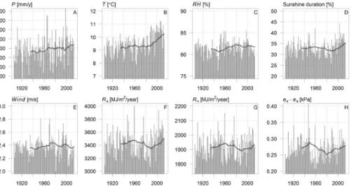
2.2 Meteorological data
We use meteorological data from De Bilt, the Netherlands, covering the period 1906–2013, which was provided by the Royal Netherlands Meteorological Institute (KNMI). De Bilt (longitude=5.177◦E, latitude
=52.101◦N, altitude
=2 m) is the main
15
meteorological site of the KNMI, located in the center of the Netherlands. Daily records are available for minimum and maximum temperature, sunshine hours, wind speed, and precipitation from 1906 onwards, and for global radiation from 1957. The observations are continuous, except for April 1945, where values from April 1944 are used instead. All required input variables are calculated for the period 1906–
20
2013 following Allen et al. (1998). Observed global radiation was used to derive the Angstrom coefficients needed to calculate daily global radiation (Allen et al., 1998) from 1906 onwards. For consistency we only use these simulated values for further analysis, which agree very well with observations (1957–2013, Radj2 =0.96). Wind speed, measured at different heights, was scaled to the reference height of
25
HESSD
11, 10787–10828, 2014How over 100 years of climate variability may affect estimates
of potential evaporation
R. P. Bartholomeus et al.
Title Page
Abstract Introduction
Conclusions References
Tables Figures
◭ ◮
◭ ◮
Back Close
Full Screen / Esc
Printer-friendly Version Interactive Discussion
Discussion
P
a
per
|
Discus
sion
P
a
per
|
Discussion
P
a
per
|
Discussion
P
a
per
|
The dataset resembles the global trends of global dimming/brightening and values of global radiation (Rs) show a similar trend to the observations for Stockholm, as presented in Wild (2009). The data (Fig. 3) show an increase in temperature consistent with previous studies (Solomon et al., 2007) and a pattern of sunshine duration consistent with dimming and brightening for northwestern Europe identified
5
by Sanchez-Lorenzo et al. (2008).
Long time series of meteorological observations will, to some extent, not be homogeneous, for example due to changes in measurement devices over time. However, this does not affect the calculations herein, as the aim is to investigate the sensitivity of the two-step potential evaporation methodology to non-stationary climate,
10
rather than to produce an exact reconstruction of the last century’s climate conditions. In this way, changes in measurement accuracy with time simply represent another non-stationary trend in this data set.
2.3 Reference evaporation
Several methods are available for calculating reference evaporation, differing in
15
complexity and empiricism (Sperna Weiland et al., 2012; Bormann, 2011; Federer et al., 1996). Here we analyze five of these methods, given in Table 1: the physically-based Penman–Monteith equation (PM), the radiation physically-based methods of Makkink (Mak) and Priestley–Taylor (PT), and the temperature based methods of Hargreaves (Har) and Blaney–Criddle (BC).
20
The FAO-56 method (Allen et al., 1998), using PM parameterized for reference grass, is recommended as the international standard for calculation ofEref. Given the physical basis of PM, it can be used globally, without the need to estimate or calibrate its parameters (Droogers and Allen, 2002). In contrast, the methods of Mak, PT, Har, and BC contain empirical coefficients, derived for specific meteorological conditions and
25
sites. Following Farmer et al. (2011) we considerEref_PM as the best approximation of Eref. In order to reduce any systematic differences between Eref values, we estimate the empirical factorsC1,C0,α′,β,a,b,c,d of the other fourE
refmethods (Table 1) by
HESSD
11, 10787–10828, 2014How over 100 years of climate variability may affect estimates
of potential evaporation
R. P. Bartholomeus et al.
Title Page
Abstract Introduction
Conclusions References
Tables Figures
◭ ◮
◭ ◮
Back Close
Full Screen / Esc
Printer-friendly Version Interactive Discussion
Discussion
P
a
per
|
Discus
sion
P
a
per
|
Discussion
P
a
per
|
Discussion
P
a
per
|
least squares regression against the simulated dailyEref_PM, for a specific calibration
period. Subsequently, daily values ofErefare calculated for each method during the full period, i.e. 1906–2013, and deviations between the empiricalErefmethods andEref_PM are calculated. The sensitivity ofEref to the choice of calibration period is evaluated for
each of the methods usingEref_PMas a basis.
5
2.4 Synthetic evaporation series
Synthetic time series of the three evaporation components are derived to systematically unravel the use of empirical crop factors. The synthetic time series are based on the physical model SWAP (Van Dam et al., 2008; Kroes et al., 2009) from whichEt,Esand Eican be simulated separately. From these simulations we derive monthlyK values for
10
eachErefmethod (5×) and vegetation class (5×) (Fig. 2: §2.5), which are subsequently
used to derive the corresponding potential evaporation components (5×5×3) using the two-step approach (Fig. 2: §2.6).
Standard values for the vegetation classes and their schematization are taken from the National Hydrologic Instrument (NHI, http://www.nhi.nu/nhi_uk.html; De Lange
15
et al., 2014) of the Netherlands. The vegetation schematization is constant throughout the period 1906–2013, i.e. dynamic vegetation is not simulated. We consider five natural vegetation classes: grassland (height=0.5 m and no full soil cover, i.e. not to be confused with the reference grass), heather, deciduous forest, pine forest and spruce forest. Parameters are chosen following NHI (2008) and are provided in the
20
Supplement. It should be noted that we do not discuss the exact validity of the parameter values used, as we are only concerned with evaporation sensitivity to non-stationary climate within the range of typical vegetation.
SWAP simulates the potential evaporation components of a crop or vegetation class based on the aerodynamic resistance, height, leaf area index (LAI), and albedo.
25
HESSD
11, 10787–10828, 2014How over 100 years of climate variability may affect estimates
of potential evaporation
R. P. Bartholomeus et al.
Title Page
Abstract Introduction
Conclusions References
Tables Figures
◭ ◮
◭ ◮
Back Close
Full Screen / Esc
Printer-friendly Version Interactive Discussion
Discussion
P
a
per
|
Discus
sion
P
a
per
|
Discussion
P
a
per
|
Discussion
P
a
per
|
Interception, which partly evaporates (Ei) and partly drips to the ground, is estimated
following Von Hoyningen-Hüne (1983) and Braden (1985) for short vegetation and Gash et al. (1995) for forests. For an extended description of SWAP and the procedures for calculatingEt,EsandEi, we refer to Kroes et al. (2009) and Van Dam et al. (2008).
Given the international recognition of the SWAP model and successful testing, we
5
assume that the model is able to produce representative synthetic estimates of each evaporation component.
As Kt and Kts are defined for a vegetated surface with a dry canopy (i.e. without interception) andKtot includes interception (see Introduction), two different SWAP runs are performed for each vegetation class, without and with interception. Throughout
10
the paper,Et andEs are valid for conditions with a dry canopy, whereas Etot includes interception and its limiting effect on transpiration and soil evaporation.
2.5 Derivation ofKt,KtsandKtot
We deriveKt,Kts and Ktot for each vegetation class (5×) andEref method (5×) based
on the syntheticEt,Es andEtot time series, and the equations given in Table 2. Similar
15
to the calibration ofErefmethods,K values are derived for a specific calibration period, (e.g. 1906–1935).K values for each vegetation class andEref method are derived as monthly averages over the calibration period.
2.6 Calculation of potential evaporation components using the two-step approach
20
Potential evaporation components,Et,Et plusEs(hereafter Et&Es) andEtot, for each vegetation class and method are calculated from the dailyEref values by multiplying it with the corresponding K values, respectively Kt, Kts and Ktot, for each vegetation class. Using these three definitions of crop factors separately allows quantifying the error that is made by correcting for each evaporation component.
25
HESSD
11, 10787–10828, 2014How over 100 years of climate variability may affect estimates
of potential evaporation
R. P. Bartholomeus et al.
Title Page
Abstract Introduction
Conclusions References
Tables Figures
◭ ◮
◭ ◮
Back Close
Full Screen / Esc
Printer-friendly Version Interactive Discussion
Discussion
P
a
per
|
Discus
sion
P
a
per
|
Discussion
P
a
per
|
Discussion
P
a
per
|
Eref estimates that are calibrated for a specific period, combined with K values
determined for the same period, are used to calculate daily values of Et, Et&Es and Etot for the full period, i.e. 1906–2013. This procedure corresponds to what is commonly done using the two-step approach, where the empirical parameters of an Erefmethod are fixed for the region in question, along with the correspondingK values.
5
Here, we determine the deviation that is potentially introduced when this approach is applied outside its calibration range (period and region/site) in a changing environment, by comparingEt(Eref,Kt), Et&Es(Eref,Kts) and Etot(Eref,Ktot) obtained by the two-step approach with the synthetic “observed”Et,Et&EsandEtot series.
3 Results 10
3.1 Calibration period and reference evaporation
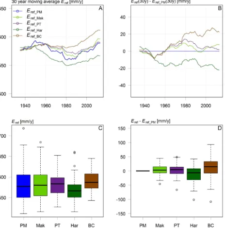
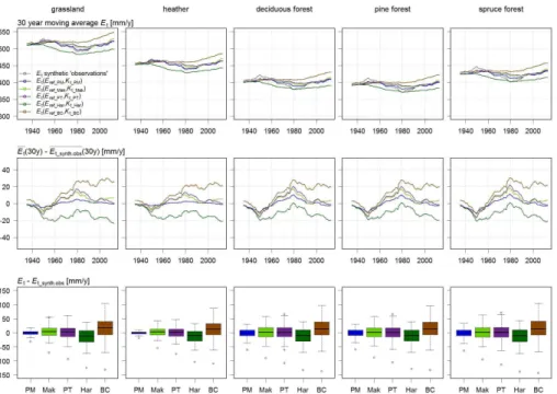
Figure 4 shows the 30 year backwards-looking moving averageEref according to PM,
Mak, PT, Har and BC, with the four latter models calibrated to fit the simulated Eref_PM for the first 30 year period, i.e. the calibration period 1906–1935. The minor differences seen between all 30 year mean Eref values during the calibration period 15
(Fig. 4a, year 1935) indicate that each method was calibrated successfully. Using the calibrated equations,Eref’s are calculated for the period 1906–2013, i.e. also outside the calibration period. All empirical models are evaluated with respect to the physically basedEref_PM, which was also used when calibrating the empirical coefficients. The radiation based methods, Mak and PT, deviate only slightly from PM on average
20
with no consistent bias (Fig. 4d), while the temperature based methods, Har and BC, deviate systematically from PM, each in different directions (Fig. 4b and d): Har consistently underestimates Eref, while BC consistently overestimates Eref. All four empirical models are unable to reproduce the extreme high evaporation values predicted by PM, especially Har and BC (Fig. 4c). The deviations from Eref_PM are
HESSD
11, 10787–10828, 2014How over 100 years of climate variability may affect estimates
of potential evaporation
R. P. Bartholomeus et al.
Title Page
Abstract Introduction
Conclusions References
Tables Figures
◭ ◮
◭ ◮
Back Close
Full Screen / Esc
Printer-friendly Version Interactive Discussion
Discussion
P
a
per
|
Discus
sion
P
a
per
|
Discussion
P
a
per
|
Discussion
P
a
per
|
considerably larger for individual years (Fig. 4d) than for the 30 year moving average (Fig. 4b).
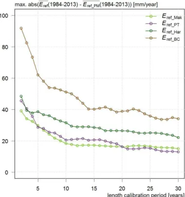
In practice, 30 year observed time series of evaporation are rarely available for calibration. Therefore, Fig. 5 shows the effect of calibration period length on estimates ofEref for the current climate (1984–2013). This effect is expressed as the maximum
5
absolute deviation of the 30 year average with respect toEref_PM. Figure 5 was compiled by first calibrating the empirical Eref coefficients for all possible calibration periods (in 1906–2013) with a given length (2–30 years) and then simulating Eref for the period 1984–2013 using the calibrated coefficients. The largest deviations occur for shorter calibration periods, as expected. Specific years may cause large deviations
10
when the obtained empirical coefficients are applied outside the calibration period. Deviation deceases notably with increasing calibration periods, suggesting that using more calibration data should result in more stable and accurateErefestimates. As the calibration period length decreases, deviations in the 30 year averageEref for 1984– 2013 increase exponentially.
15
It should be noted that only deviations in 30 year averages are shown for varying calibration period lengths; deviations in the underlying yearly values are larger, as indicated by Fig. 4d. Additionally, the amplitude of the deviations shown in Fig. 4b and d would increase when calibrated using periods shorter than 30 years (Fig. 5).
3.2 Crop factors and potential evaporation components 20
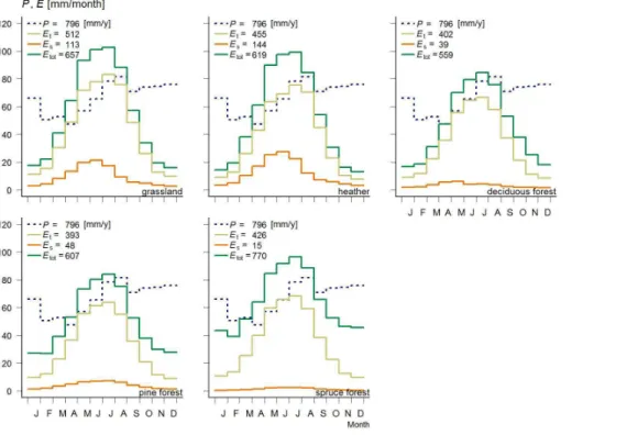
Figure 6 gives monthly average synthetic evaporation componentsEt,EsandEtotwhich were used to derive monthly crop factors (three methods: Table 2) for five vegetation classes and fiveEref methods (Table 1), i.e. 3×5×5 crop factors for each calibration
period. In contrast to the reference grass surface, the grassland of Fig. 6 does not fully cover the soil, which results in higherEs and lower Et. Figure 7 shows simulated
25
Et (the two-step approach) for the period 1906–2013, using empirical coefficients for each Eref method and matching Kt values, all calibrated on the period 1906–1935. The general patterns in Et correspond to those of Eref (Fig. 4b), meaning that the
HESSD
11, 10787–10828, 2014How over 100 years of climate variability may affect estimates
of potential evaporation
R. P. Bartholomeus et al.
Title Page
Abstract Introduction
Conclusions References
Tables Figures
◭ ◮
◭ ◮
Back Close
Full Screen / Esc
Printer-friendly Version Interactive Discussion
Discussion
P
a
per
|
Discus
sion
P
a
per
|
Discussion
P
a
per
|
Discussion
P
a
per
|
deviations introduced by the two-step approach are mainly determined by the empirical coefficients in theErefmethods.
The deviation introduced for Et derived from Eref_PM and Kt_PM is relatively minor compared to what is found for the empirical Eref methods, especially for short vegetation. Apparently,Eref_PMfollows the trend inEt(also obtained using the Penman–
5
Monteith equation, but parameterized for each vegetation class, Sect. 2.4) and the ratio ofEt andEref_PM, used to estimateKt_PM, changes little with time for short vegetation. More significant effects of Kt_PM are seen for taller vegetation, as climate induced temporal changes in Eref_PM show a height dependent nonlinear relation to changes in Et (Allen et al., 1998). Therefore, the deviation introduced when using Eref_PM is
10
larger for forests than for the short vegetation classes (Fig. 7). Similar to what is seen in Fig. 4, the deviations for individual years can be considerably larger than the climatic averages.
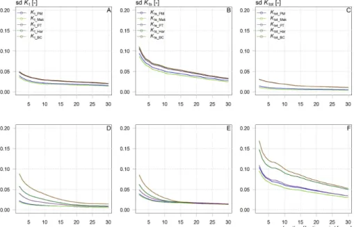
Figure 8 shows the sensitivity of crop factors,K, with respect to the calibration period length for heather and spruce forest. The variation in K decreases with increasing
15
calibration length for all methods, but, except forEref_Mak, the variability ofK values for the empiricalEref methods is larger than forEref_PM. These differences are especially notable for forests and illustrate that a poor relationship between theEref method and the synthetic potential evaporation component (Sect. 2.4) is compensated byK values that thus show a larger variation over time. Remarkable is the low variability in Ktot
20
values for heather (Fig. 8c), which indicates that the variability seen for Kt (Fig. 8a)
is reduced by interception. However, for spruce forest, for which interception is much more dominant, interception increases the variability inKtot.
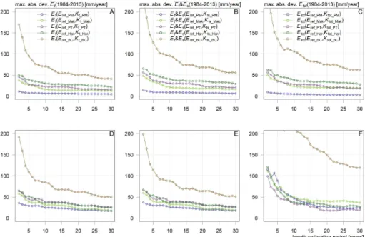
From Fig. 8a and d, it can be concluded that the deviations shown in Fig. 7 will increase when shorter calibration periods are used, irrespective of the applied Eref
25
method. Figure 9 shows the effect of period (years and length) on the maximum absolute deviation made by the two-step approach for each Eref method and for
HESSD
11, 10787–10828, 2014How over 100 years of climate variability may affect estimates
of potential evaporation
R. P. Bartholomeus et al.
Title Page
Abstract Introduction
Conclusions References
Tables Figures
◭ ◮
◭ ◮
Back Close
Full Screen / Esc
Printer-friendly Version Interactive Discussion
Discussion
P
a
per
|
Discus
sion
P
a
per
|
Discussion
P
a
per
|
Discussion
P
a
per
|
shorter calibration periods are used. Additionally, Fig. 9 illustrates that deviations are (i) larger for tall vegetation than for short vegetation and (ii) larger forKtot than forKt and Kts for vegetation classes with high interception, as is the case for spruce forest. The large deviations forEtot for spruce forest confirm the remark by De Bruin and Lablans
(1998), that for wet forest evaporation, the crop factor approach will not be sufficient.
5
Nevertheless, when derived for a sufficiently long time series, the deviations level out and there is no detectable bias.
4 Discussion
4.1 Temporal robustness in hydrological modeling
In this paper we systematically unraveled how empirical coefficients in the
two-10
step approach affect estimates of potential evaporation. We used the past century’s time series of observed climate containing non-stationary signals of multi-decadal atmospheric oscillations, global warming, and global dimming/brightening (Suo et al., 2013; Stanhill, 2007; Wild, 2009; Wild et al., 2005) to evaluate the sensitivity of the two-step approach to both the length of the reference calibration period and the reference
15
years. To this end we calibrated the empirical coefficients of the two-step approach based on different periods and then showed that using the thus obtained empirical coefficients outside their calibration range may lead to systematic differences between Erefmethods, and to systematic errors in estimated potentialEcomponents. The signs of the errors for calculated climatic average evaporation components differ, depending
20
on theEref method used, and on the specific period (length and years) of calibration. Hooghart and Lablans (1988) stated that, for the two-step approach, the correctness of empirical coefficients for the estimation of Eref are of minor importance, as these are compensated by K. However, here we have shown that while this may be true within the calibration period, this statement does not hold when extrapolating. As
25
potential evaporation is a key input in hydrological models, input errors will propagate
HESSD
11, 10787–10828, 2014How over 100 years of climate variability may affect estimates
of potential evaporation
R. P. Bartholomeus et al.
Title Page
Abstract Introduction
Conclusions References
Tables Figures
◭ ◮
◭ ◮
Back Close
Full Screen / Esc
Printer-friendly Version Interactive Discussion
Discussion
P
a
per
|
Discus
sion
P
a
per
|
Discussion
P
a
per
|
Discussion
P
a
per
|
to estimates of related processes, such as the soil moisture budget, droughts, recharge and groundwater processes.
Although this result may seem trivial, the two-step approach, including extrapolating empirical coefficients, is common practice in hydrological modeling, as mentioned in the introduction. Ehret et al. (2014) state that “in hydrological modeling, it
5
is often conveniently assumed that the variables presenting climate vary in time while the general model structure and model parameters representing catchment characteristics remain time-invariant”. There is a clear parallel of this statement with the approach presented herein where meteorological conditions vary in time, while climate-dependent (empirical) parameters are often fixed values.
10
In practice, long time series of observed evaporation are rare and not evenly distributed spatially. As such, for many applications, hydrologists must rely on incomplete calibration data, use analogous stations with similar characteristics, or simply default to published values for crop factors and Eref model parameters. This study has shown that potential evaporation estimates are most accurate and stable
15
with a long calibration period. However, even when using a long observed record, estimates may include errors due to the assumption of constant empirical coefficients in a non-stationary climate, i.e. the calibration period not being representative of current conditions. Evaporation estimates outside the calibration period are even more susceptible to non-stationarity when the calibration period is relatively short, as with
20
areas where observed evaporation data are sparse. Finally, estimating evaporation based on published typical values without calibration is most susceptible to errors, as these parameters are typically global averages but also contain the non-stationary reference period issues identified in this paper. To remove bias by systematic input errors, as in e.g. evaporation, it is common practice to tune models by calibration,
25
non-HESSD
11, 10787–10828, 2014How over 100 years of climate variability may affect estimates
of potential evaporation
R. P. Bartholomeus et al.
Title Page
Abstract Introduction
Conclusions References
Tables Figures
◭ ◮
◭ ◮
Back Close
Full Screen / Esc
Printer-friendly Version Interactive Discussion
Discussion
P
a
per
|
Discus
sion
P
a
per
|
Discussion
P
a
per
|
Discussion
P
a
per
|
constant bias occurs for bothErefand potentialEestimates, thus limits their application
outside the calibration range.
4.2 Propagation of dimming/brightening periods
In contrast to Fig. 9, which only shows the maximum absolute deviations for the 30 year average potential evaporation components for the years 1984–2013 as a function of
5
the calibration period length, Fig. 10 includes the results of all underlying deviations for heather and spruce usingEref_PT. Figure 10 demonstrates that climate variability induces systematic overestimation or underestimation of the calculated potential evaporation components, depending on the calibration period used. The sign of the error strongly varies with the calibration period, and the inclusion of a single anomalous
10
year can change the sign of the error.
Figure 10 further shows that anomalous years or multi-annual climate patterns tend to propagate considerable errors outside the calibration period to the current climate (1984–2013). The patterns of deviations from the synthetic “observations” show similarities to the global dimming and brightening periods (see Introduction):
15
the first warming period (about 1925–1945) causes a systematic overestimation up to calibration lengths of 30 years, although specific calibration years may result in an underestimation for shorter calibration lengths. The succeeding period of cooling leads to a systematic overestimation, while the second warming period (starting around 1975) results in a more variable pattern. The latter may be linked to the finding of Wang
20
and Dickinson (2013) that, in contrast to the years until the 1970’s, there is no significant relationship between variations in temperature and global radiation in following years.
The patterns are comparable for Et, Et&Es and Etot, based on Kt, Kts and Ktot respectively, for short vegetation classes. However, for tall vegetation classes with high interception capacity, e.g. spruce (Fig. 10f), usingKtot results in a more noisy pattern
25
due to specific years of high precipitation. Additionally, including interception may shift the sign of the error.
HESSD
11, 10787–10828, 2014How over 100 years of climate variability may affect estimates
of potential evaporation
R. P. Bartholomeus et al.
Title Page
Abstract Introduction
Conclusions References
Tables Figures
◭ ◮
◭ ◮
Back Close
Full Screen / Esc
Printer-friendly Version Interactive Discussion
Discussion
P
a
per
|
Discus
sion
P
a
per
|
Discussion
P
a
per
|
Discussion
P
a
per
|
4.3 Implications for climate change impact studies
Poor transferability of parameter estimates made during calibration can have potentially large impacts for studies in non-stationary conditions (Coron et al., 2014), e.g. for climate change impact studies (Bormann, 2011; Karlsson et al., 2014). To improve the temporal robustness of hydrological modeling, Coron et al. (2014) propose, while
5
putting it in the framework of the new IAHS Scientific Decade “Panta Rhei” (Montanari et al., 2013), to particularly advance in the ability to estimate temporal variations in evaporation fluxes. This study contributes to this larger objective.
For climate change impact studies, applications of empirical models are particularly problematic, as empirical methods closely approximate observations of natural
10
processes, but do not capture the underlying physics. When extrapolating to new climate regimes, these assumption are not guaranteed to remain valid (Kay and Davies, 2008; Bormann, 2011; Arnell, 1999). Similar to our findings, simulating historic non-stationary climatic conditions, Kay and Davies (2008) demonstrate that Eref_PM and temperature based Eref methods give different projected evaporation estimates when
15
applied to future climate model data. Additionally, Haddeland et al. (2011) show, using the WATCH climate forcing data (Weedon et al., 2011), that global hydrological models that differ in their choice of evaporation schemes, show significantly different evaporation estimates. These large discrepancies in an important part of the water cycle may have a large effect on the modeled hydrological impacts of climate change
20
and increases the uncertainty of impact estimates (Bormann, 2011; Kay and Davies, 2008; Haddeland et al., 2011).
To show the implications of using different empirical Eref methods in hydrological applications under recent climate change, without the need for numerous extensive model runs, we calculated the Standardized Precipitation and Evaporation Index (SPEI)
25
HESSD
11, 10787–10828, 2014How over 100 years of climate variability may affect estimates
of potential evaporation
R. P. Bartholomeus et al.
Title Page
Abstract Introduction
Conclusions References
Tables Figures
◭ ◮
◭ ◮
Back Close
Full Screen / Esc
Printer-friendly Version Interactive Discussion
Discussion
P
a
per
|
Discus
sion
P
a
per
|
Discussion
P
a
per
|
Discussion
P
a
per
|
The SPEI (Beguería et al., 2013; Vicente-Serrano et al., 2010) is a commonly used meteorological drought index, which is a variant of the WMO-recommended Standardized Precipitation Index SPI (Guttman, 1999; Hayes et al., 2011; McKee et al., 1993). Unlike the SPI, which calculates precipitation accumulated over a period and then normalizes the accumulated value based on typical seasonal conditions, the SPEI
5
instead normalizes the accumulated difference of the climatic water balance, defined as the difference between precipitation andEref. This produces a time series of normalized values, such that an SPEI of 0 refers to typical conditions, an SPEI of negative one refers to a condition whereΣ(P −Eref) is one standard deviation drier than typical, and
vice versa for positive one. For this example, the SPEI6 was calculated, normalizing
10
the climatic water balance summed over the preceding six months, following the fitting procedures outlined in Stagge et al. (2014a) and Gudmundsson and Stagge (2014).
Figure 11 shows the results of this analysis, with the assumed accurate SPEI6, based on Eref_PM, shown at the top and the difference between this and SPEI6 for all other empirical reference evaporation models shown below. As with the results of
15
Erefsimulations, the Mak and PT models are closest to the observed signal (differences in the range of−0.2 to 0.2), while the Har and BC models produce greater variability (∆SPEI6=−0.5 to 0.5). Differences of this magnitude can make a large difference when interpreting drought risk. For example, the year 1947 produced a severe drought at the De Bilt site (SPEI6=−2.2); however all other methods underestimate
20
Eref, producing SPEI6 values between −1.5 and −1.9. This in turn, changes the interpretation of this drought from an event expected to occur once every 72 years to an event expected to occur once every 15–35 years. This is a significant difference in risk level which can be attributed to differences among the evaporation methods and a potentially non-representative calibration period. SPEI sensitivity to Eref method is
25
analyzed in greater detail in Stagge et al. (2014b).
HESSD
11, 10787–10828, 2014How over 100 years of climate variability may affect estimates
of potential evaporation
R. P. Bartholomeus et al.
Title Page
Abstract Introduction
Conclusions References
Tables Figures
◭ ◮
◭ ◮
Back Close
Full Screen / Esc
Printer-friendly Version Interactive Discussion
Discussion
P
a
per
|
Discus
sion
P
a
per
|
Discussion
P
a
per
|
Discussion
P
a
per
|
5 Conclusion
In this study we thoroughly analyzed the robustness of the two-step approach to simulate potential evaporation. We show that systematic errors may be introduced when empirical coefficients are applied outside their calibration period, and that the magnitude of these errors depends on the period and length of the calibration period.
5
With our analysis, we want to raise awareness of possible systematic errors that may be introduced in estimates of potential evaporation and in hydrological modeling studies due to straightforward application of (i) the common two-step approach for potential evaporation specifically, and (ii) fixed instead of time-variant model parameters in general.
10
The Supplement related to this article is available online at doi:10.5194/hessd-11-10787-2014-supplement.
Acknowledgements. This study was carried out under the auspices of the joint research program of the Dutch Water Utility sector.
References 15
Abbott, M. B., Bathurst, J. C., Cunge, J. A., O’Connell, P. E., and Rasmussen, J.: An introduction to the European Hydrological System – Systeme Hydrologique Europeen, “SHE”, 2: structure of a physically-based, distributed modelling system, J. Hydrol., 87, 61–77, 1986.
Allen, R. G.: Using the FAO-56 dual crop coefficient method over an irrigated region as part of an evapotranspiration intercomparison study, J. Hydrol., 229, 27–41, 2000.
20
Allen, R. G. and Pruitt, W. O.: Rational use of the FAO Blaney–Criddle formula, J. Irrig. Drain. E.-ASCE, 112, 139–155, 1986.
Allen, R. G., Pereira, L. S., Raes, D., and Smith, M.: Crop Evapotranspiration: Guidelines for Computing Crop Water Requirements (FAO irriggation and drainage paper), Food and Agriculture Organization of the United Nations, Rome, 1998.
HESSD
11, 10787–10828, 2014How over 100 years of climate variability may affect estimates
of potential evaporation
R. P. Bartholomeus et al.
Title Page
Abstract Introduction
Conclusions References
Tables Figures
◭ ◮
◭ ◮
Back Close
Full Screen / Esc
Printer-friendly Version Interactive Discussion
Discussion
P
a
per
|
Discus
sion
P
a
per
|
Discussion
P
a
per
|
Discussion
P
a
per
|
Allen, R. G., Pereira, L. S., Smith, M., Raes, D., and Wright, J. L.: FAO-56 dual crop coefficient method for estimating evaporation from soil and application extensions, J. Irrig. Drain. E.-ASCE, 1, 2–13, 2005.
Allen, R. G., Pereira, L. S., Howell, T. A., and Jensen, M. E.: Evapotranspiration information reporting: I. Factors governing measurement accuracy, Agr. Water. Manage., 98, 899–920, 5
doi:10.1016/j.agwat.2010.12.015, 2011.
Andréassian, V., Perrin, C., and Michel, C.: Impact of imperfect potential evapotranspiration knowledge on the efficiency and parameters of watershed models, J. Hydrol., 286, 19–35, 2004.
Arnell, N. W.: The effect of climate change on hydrological regimes in Europe: a continental 10
perspective, Global Environ. Chang., 9, 5–23, doi:10.1016/S0959-3780(98)00015-6, 1999. Beguería, S., Vicente-Serrano, S. M., Reig, F., and Latorre, B.: Standardized Precipitation
Evap-otranspiration Index (SPEI) revisited: Parameter fitting, evapEvap-otranspiration models, tools, datasets and drought monitoring, Int. J. Climatol., 34, 3001–3023, doi:10.1002/joc.3887, 2013.
15
Bergström, S. and Forsman, A.: Development of a conceptual deterministic rainfall–runoff
model, Nord. Hydrol., 4, 147–170, 1973.
Blaney, H. F. and Criddle, W. P.: Determining Water Requirements in Irrigated Areas From Climatological and Irrigation Data, USDA (SCS), Washington, D.C., 48, 1950.
Bormann, H.: Sensitivity analysis of 18 different potential evapotranspiration models to 20
observed climatic change at German climate stations, Climatic Change, 104, 729–753, doi:10.1007/s10584-010-9869-7, 2011.
Braden, H.: Ein Energiehaushalts- und Verdunstungsmodell for Wasser und Stoff haushalt-suntersuchungen landwirtschaftlich genutzer Einzugsgebiete, Mittelungen Deutsche Bodenkundliche Geselschaft, 42, 294–299, 1985 (in German).
25
Bradford, R. B., Ragab, R., Crooks, S. M., Bouraoui, F., and Peters, E.: Simplicity versus complexity in modelling groundwater recharge in Chalk catchments, Hydrol. Earth Syst. Sci., 6, 927–937, doi:10.5194/hess-6-927-2002, 2002.
Calder, I. R.: Assessing the water use of short vegetation and forests: development of the Hydrological Land Use Change (HYLUC) model, Water Resour. Res., 39, 1318, 30
doi:10.1029/2003wr002040, 2003.
Coron, L., Andréassian, V., Perrin, C., Bourqui, M., and Hendrickx, F.: On the lack of robustness of hydrologic models regarding water balance simulation: a diagnostic approach applied to
HESSD
11, 10787–10828, 2014How over 100 years of climate variability may affect estimates
of potential evaporation
R. P. Bartholomeus et al.
Title Page
Abstract Introduction
Conclusions References
Tables Figures
◭ ◮
◭ ◮
Back Close
Full Screen / Esc
Printer-friendly Version Interactive Discussion
Discussion
P
a
per
|
Discus
sion
P
a
per
|
Discussion
P
a
per
|
Discussion
P
a
per
|
three models of increasing complexity on 20 mountainous catchments, Hydrol. Earth Syst. Sci., 18, 727–746, doi:10.5194/hess-18-727-2014, 2014.
De Bruin, H. A. R. and Holtslag, A. A. M.: A simple parameterization of the surface fluxes of sensible and latent heat during daytime compared with the Penman–Monteith concept, J. Appl. Meteorol., 21, 1610–1621, doi:10.1175/1520-0450(1982)021<1610:aspots>2.0.co;2, 5
1982.
De Bruin, H. A. R. and Lablans, W. N.: Reference crop evapotranspiration determined with a modified Makkink equation, Hydrol. Process., 12, 1053–1062, 1998.
De Lange, W. J., Prinsen, G. F., Hoogewoud, J. C., Veldhuizen, A. A., Verkaik, J., Oude Essink, G. H. P., van Walsum, P. E. V., Delsman, J. R., Hunink, J. C., Massop, H. T. L., and 10
Kroon, T.: An operational, multi-scale, multi-model system for consensus-based, integrated water management and policy analysis: the Netherlands Hydrological Instrument, Environ. Modell. Softw., 59, 98–108, doi:10.1016/j.envsoft.2014.05.009, 2014.
Doorenbos, J. and Pruitt, W. O.: Crop water requirements; irrigation and drainage paper no. 24, FAO, Rome, 1977.
15
Driessen, T. L. A., Hurkmans, R. T. W. L., Terink, W., Hazenberg, P., Torfs, P. J. J. F., and Uijlenhoet, R.: The hydrological response of the Ourthe catchment to climate change as modelled by the HBV model, Hydrol. Earth Syst. Sci., 14, 651–665, doi:10.5194/hess-14-651-2010, 2010.
Droogers, P. and Allen, R. G.: Estimating reference evapotranspiration under inaccurate data 20
conditions, Irrigation and Drainage Systems, 16, 33–45, doi:10.1023/a:1015508322413, 2002.
Ehret, U., Gupta, H. V., Sivapalan, M., Weijs, S. V., Schymanski, S. J., Blöschl, G., Gelfan, A. N., Harman, C., Kleidon, A., Bogaard, T. A., Wang, D., Wagener, T., Scherer, U., Zehe, E., Bierkens, M. F. P., Di Baldassarre, G., Parajka, J., van Beek, L. P. H., van Griensven, A., 25
Westhoff, M. C., and Winsemius, H. C.: Advancing catchment hydrology to deal with predictions under change, Hydrol. Earth Syst. Sci., 18, 649–671, doi:10.5194/hess-18-649-2014, 2014.
Farmer, W., Strzepek, K., Schlosser, C. A., Droogers, P., and Gao, X.: A method for calculating reference evapotranspiration on daily time scales, MIT Joint Program on the Science and 30
HESSD
11, 10787–10828, 2014How over 100 years of climate variability may affect estimates
of potential evaporation
R. P. Bartholomeus et al.
Title Page
Abstract Introduction
Conclusions References
Tables Figures
◭ ◮
◭ ◮
Back Close
Full Screen / Esc
Printer-friendly Version Interactive Discussion
Discussion
P
a
per
|
Discus
sion
P
a
per
|
Discussion
P
a
per
|
Discussion
P
a
per
|
Feddes, R. A.: Crop factors in relation to Makkink reference-crop evapotranspiration, in: Evaporation and Weather, Proceedings and Information., edited by: Hooghart, C., Comm. Hydrological Research TNO, The Hague, 33–47, 1987.
Feddes, R. A. and Lenselink, K. J.: Evapotranspiration, in: Drainage principles and applications, edited by: Ritzema, H. P., International Institute for Land Reclamation and Improvement ILR, 5
Wageningen, 1994.
Federer, C. A., Vörösmarty, C., and Fekete, B.: Intercomparison of methods for calculating potential evaporation in regional and global water balance models, Water Resour. Res., 32, 2315–2321, doi:10.1029/96wr00801, 1996.
Gash, J. H. C., Lloyd, C. R., and Lachaud, G.: Estimating sparse forest rainfall interception with 10
an analytical model, J. Hydrol., 170, 79–86, 1995.
Gudmundsson, L. and Stagge, J. H.: SCI: Standardized Climate Indices such as SPI, SRI or SPEI. R package version 1.0-1, ETH, Zurich, Switzerland, 2014.
Guerschman, J. P., Van Dijk, A. I. J. M., Mattersdorf, G., Beringer, J., Hutley, L. B., Leuning, R., Pipunic, R. C., and Sherman, B. S.: Scaling of potential evapotranspiration with MODIS data 15
reproduces flux observations and catchment water balance observations across Australia, J. Hydrol., 369, 107–119, doi:10.1016/j.jhydrol.2009.02.013, 2009.
Guttman, N. B.: Accepting the Standardized Precipitation Index: a Calculation Algorithm, Wiley Online Library, 1999.
Haddeland, I., Clark, D. B., Franssen, W., Ludwig, F., Voß, F., Arnell, N. W., Bertrand, N., 20
Best, M., Folwell, S., Gerten, D., Gomes, S., Gosling, S. N., Hagemann, S., Hanasaki, N., Harding, R., Heinke, J., Kabat, P., Koirala, S., Oki, T., Polcher, J., Stacke, T., Viterbo, P., Weedon, G. P., and Yeh, P.: Multimodel estimate of the global terrestrial water balance: setup and first results, J. Hydrometeorol., 12, 869–884, doi:10.1175/2011jhm1324.1, 2011. Hayes, M., Svoboda, M., Wall, N., and Widhalm, M.: The lincoln declaration on drought indices: 25
universal meteorological drought index recommended, B. Am. Meteorol. Soc., 92, 485–488, doi:10.1175/2010BAMS3103.1, 2011.
Hooghart, J. C. and Lablans, W. N.: Van Penman naar Makkink: Een nieuwe berekeningswijze voor de klimatologische verdampingsgetallen, KNMI, De Bilt, 1988 (in Dutch).
Hupet, F. and Vanclooster, M.: Effect of the sampling frequency of meteorological
30
variables on the estimation of the reference evapotranspiration, J. Hydrol., 243, 192–204, doi:10.1016/S0022-1694(00)00413-3, 2001.
![Table 1. Equations used to calculate daily values of reference evaporation E ref [mm d −1 ] for the period 1906–2013 at De Bilt meteorological station.](https://thumb-eu.123doks.com/thumbv2/123dok_br/16482740.199982/30.918.70.674.234.402/table-equations-calculate-values-reference-evaporation-meteorological-station.webp)