ELECTRICAL AGEING STUDIES OF POLYMERIC INSULATION FOR POWER CABLES (ESTUDO DO ENVELHECIMENTO ELECTRICO DO ISOLANTE POLIMERICO DE CABOS ELECTRICOS)

MARIA DO

CARMO

HENRIQUES

LAN~A

ELECTRICAL AGEING STUDIES OF POLYMERIC

INSULATION FOR POWER CABLES

(ESTUDO DO ENVELHECIMENTO ELECTRICO

DO ISOLANTE POLIMERICO DE

CABOS ELECTRICOS)

Dissertacao apresentada para obtencao do

Grau de Doutor em Engenharia Fisica -Fisica Aplicada pela Universidade Nova de Lisboa, Faculdade de Ciencias e Tecnologia.

LISBOA

To the late Dilip Das Gupta

and

A

mem6ria de minha mae,

Acknowledgements

Itis not an easy task to thank. all and forget none of the many that help me to do and conclude this work. There is always the danger of forgetting some. So I start by thanking those that I might have forgotten to mention and deserve to have their names here.

First, Professor Marat Mendes, my Portuguese supervisor who was always available to help me workwise, and also for his personal kindness and support in all the difficult moments.

The late Dr. Dilip Das Gupta, my British supervisor, for accepting to supervise the research work carried out at Bangor and for all the months that I stayed there. For his suggestions, ideas and keeping me on the right track and also for his personal support. Unfortunately Dilip left us before the conclusion of this thesis and he was sorely missed during the later stages of the writing.

To Professor Eugen Neagu for the many hours spend around the setup in the laboratory (for discovering what was wrong with the electrometer), for the enlightening discussions and ideas. Also for all the helpful experience of polymeric insulators, thank. you.

All in my research group in Seccao de Materiais Electroactivos of Departamento de Ciencia dos Materiais da Faculdade de Ciencias e Tecnologia da Universidade Nova de Lisboa:

Carlos Dias for the time spent helping with some experiments, and for his availability to answer any of my questions,

Professor Maria Amalia Bento, Professor Jose Marat-Mendes, Carlos Dias, Rui Igreja and Paulo Inacio for helping to ease my teaching load.

Our secretary Dina, who brighten the days with her good mood.

iv

I am also grateful to everybody I met in the laboratory of Professor Das Gupta in Bangor. To Pablo Marin-Franch for teaching me my way around the labs.

To Walter Sakamoto, especially for helping me to perform the medium frequency DRS measurements with the lock-in amplifier and for keeping me in touch with the Portuguese language.

To Albert Rees with all his technical knowledge always available to give a helping hand or to find someone that could do it.

A special thanks to Claudia Castellani and Yener Altunbas for their friendship, all the encouraging words and nice dinners making me feel part of their family. And to all the others that helped me and made me feel at home. And last but not the least to my friends Teresa Marat-Mendes and Luisa Moreno.

To Dr. Paulo Scarpa, sadly deceased, for his thesis that helped me to start to understand the meaning of electrical ageing and polymeric insulation. For being always available to do some measurements and answer my many questions.

I do not want to forget the place where this work started, in Professor Robert Hill's laboratory at Kings College in London, where I had the pleasure of working with Professor Len Dissado (now at Leicester University) on the fractal nature of water trees. I am also grateful to John Alison and Leslie Askew for helping during my stay there.

I am also very grateful to Professor John Fothergill and John Houlgreave at Leicester University for lending me the first modified Cigre cells that I used for ageing. Also once more to Professor Len Dissado, Dr. Kaori Fukunaga, Alex See and Will Peasgood for the PEA measurements and discussion of results.

I would like to thank Fundacao Calouste Gulbenkian for the financial support that allowed me to travel to the University of Bangor.

I am in debt to Eng. Francisco Pedroso of General Cable, CelCat, who has provided us with the polyester films for pressing and who has always been always available to sort out any problems.

Warm thanks to my friends for listening and bearing with me at all my troubled and difficult moments. Thank you to Paulo Ivo Teixeira for helping to correct the English. And especially to my friend Jose Esteves for all the help with Linux and availability to solve any small or big computer stuff problem.

vi

Resumo

Os polimeros tern sido extensivamente usados como isolantes em cabos electricos, 0 polietileno, primeiro polietileno de baixa densidade e mais recentemente na sua forma reticulada, e urn dos isolantes mais comuns em cabos electricos de media e alta tensao. Este dielectrico sofre de envelhecimento electrico sob diferentes formas, tais como arborescencias

de agua e electricas e por fim rupturadielectrica,0 ultimo processo leva a dispendiosas falhas

dos cabos electricos, Muitos trabalhos de investigacao tern sido dedicados a este assunto e,

apesar do progresso feito, os resultados sao muitas vezes contradit6rios e diffceis de

reproduzir. Qualquer nova informacao sobre este problema

e

urn passo em frente na

prevencao da falha dos cabos e na aumento do seu tempo de vida titil.

o

objectivo desta tese

e

relacionar dois aspectos diferentes do envelhecimento electrico: dano

localizado e mudancas nas propriedades de volume do polietileno. Para tentar alcancar este objectivo diferentes tecnicas experimentais tiveram de ser usadas. 0 dana localisado

apresenta-se sob a forma de arborescencias de agua (water trees) e canais de ruptura

dielectrica, uma vez que arborescencias electricas (electrical trees) nao foram observadas no

decurso deste trabalho. Os metodos usados neste estudo foram FfIR, determinacao da dimensao fractal de arborescencias de agua e estatfstica da ruptura dielectrics. As

modificacoes das propriedades electricas e dielectricas de volume foram obtidas,

principalmente, por DRS, FfSDC e PEA. A partir dos resultados de ¥fIR foi possfvel

encontrar produtos de oxidacao (sendo os principais acetonas e ices carboxilato) e quebra de

cadeias. Os valores estimados para a dimensao fractal revelam como responsavel 0 mesmo

mecanismo microsc6pico para as arborescencias de agua (pelo menos para as envelhecidas a diferentes frequencies e temperaturas). A estatfstica da ruptura dielectrica mostra a

importancia do fabrico e processamento do isolante, uma vez que ruptura ocorrida durante 0

periodo inicial

e

maioritariamente dependente dos defeitos existentes antes do

envelhecimento. A comparacao entre os resultados de DRS, FfSDC e PEA revela 0 papel

desempenhado pela carga espacial no envelhecimento para perfodos mais longos. Os dois diferentes aspectos (envelhecimento localizado e em volume) sao diffceis de relacionar

porque 0 primeiro tern urn caracter estocastico. Contudo a presenca de carga espacial

encontrada nos estudos de volume pode ser vista como urn dos factores responsavel pelo

Summary

Polymers have been widely used as electrical insulators in power cables. Polyethylene, initially low density and more recently crosslinked, are one of the more commonly used insulators in medium and high voltage power cables. They suffer electrical ageing in different forms, such as water treeing, electrical treeing and finally dielectric breakdown. The last one leading to costly cable failure. Many research works have been developed on this subject despite of the progress made up to now, results are still sometimes contradictory and difficult to reproduce. Any new insight into this problem is a step further in preventing failure of the cables and increasing their useful lifetime.

2.1 2.1.1

2.1.2

2.1.3

2.1.4

2.1.5

3.1

3.2

3.3 3.3.1

IX

Table of contents

Chapter 1. Introduction 1

Chapter 2. Polyethylene: polymer properties 7

Polymers 7

Types of polymers 8

Bonds and structure 10

Morphology and crystallinity 11

Mechanical properties 14

Relaxation processes in polymers 15

2.2 Polyethylene 17

2.2.1 General properties 17

2.2.2 LDPE and XLPE 18

2.2.3 Voids, cavities and water in unaged polyethylene 21

2.2.4 Relaxation processes in polyethylene 22

Chapter 3. Charge transport and trapping mechanisms in insulators 25

Introduction 25

Band theory 26

Conduction and transport 29

Carrier type 30

3.3.1.1 Ionic conduction 30

3.3.1.2 Electronic conduction 32

3.3.2 Electric field 33

3.3.2.1 Low field effects 34

3.3.2.2 High field effects 35

3.4 Transient response 39

3.5 Steady state response 41

3.6 Surface conduction 42

3.7 Charge transport and trapping in polyethylene 42

Chapter 4. Dielectric relaxation 47

4.2 4.3 4.4 4.4.1 4.4.2 4.4.3

Dipolesin a static field 48

Dielectric response in time and frequency domains 49

Debye model and related empirical models 52

Debye model 52

Distribution of relaxation times 53

Related empirical models 54

4.7 4.8.3 4.8 4.8.1 4.5 4.6 4.6.1 4.6.2 4.6.3 4.6.4

Temperature dependence 56

Presentation of dielectric data 57

Parallel and series circuits 58

Cole-Cole plots 59

Displaying dielectric relaxation data 60

Temperature dependent graphs 61

Main classes of dielectric solid materials 63

Physical models 68

Jonschers Universal Law 68

4.8.1.1 General description of ''universal'' fractional power law 69

4.8.1.2 Physical interpretation of universality 70

4.8.2 Physical model: Dissado-Hill cluster model 72

4.8.2.1 Dipolar systems 73

4.8.2.2 Charge carriers systems 75

4.8.2.3 Fractal character of dielectric relaxation 77

A probabilistic model 78

4.9 Correlation between TSDC measurements and dielectric measurements 80

4.10 Dielectric relaxation processes in polyethylene: a review of experimental results _ 82

5.1 5.1.1 5.1.2 5.1.3 5.1.4 5.1.5

Chapter 5. Electrical ageing of insulating polymers 87

Water treeing 87

Morphology 88

Characteristics 90

Factors affecting initiation and growth processes 91

Oxidation and FfIR analysis 93

xi

Electrical treeing 102

Dielectric breakdown 105

Thermal breakdown 106

Electromechanical breakdown 106

Electronic breakdown 107

Partial discharge breakdown 107

Stochastic nature of breakdown 108

The influence of trapped space charge in electrical ageing 108

Chapter 6. Experimental 111

5.2 5.3 5.3.1 5.3.2 5.3.3 5.3.4 5.3.5

5.4

6.1 6.1.1 6.1.2 6.2 6.3

Sample preparation and electrical ageing 111

Usual procedure 111

Sample ageing for NMR studies (of pore dimension) 114

Analysis of the unaged polyethylene specimens, 114

Dielectric permittivity measurements, 117

6.4 Isothermal charge and discharge currents and non-isothermal discharge currents 118 Pulsed electroacoustic space charge profIle measurements (PEA) 121

Water treeing dyeing and counting 125

Fractal analyses of water trees 126

Water tree images: methylene blue and SEM microphotographs 126

Image processing and estimation of the fractal dimension 128

Chemical changes in aged polyethylene 131

FfIR studies 131

NMR studies 132

Breakdown statistics, 132

Chapter 7. Results and discussion 135

6.8 6.8.1 6.8.2 6.9 6.5 6.6 6.7 6.7.1 6.7.2

7.1 Analysis of the unaged polymer morphology and composition characteristics __ 135

7.1.1 Optical microscopy 135

7.1.2 Scanning electron microscopy (SEM) 136

7.1.3 Atomic force microscopy (AFM) 136

7.1.4 Differential scanning calorimetry (DSC) 140

7.1.6

7.2

7.2.1 7.2.2

X-ray diffraction. 144

Dielectric relaxation spectroscopy 146

Results 146

Discussion 147

7.3 Isothermal charge and discharge currents and non-isothermal discharge currents 171

7.3.1 Influence of charging/discharging conditions on reproducibility and analysis 172

7.3.2 Results and discussion 179

7.3.2.1 Unaged LDPE 180

7.3.2.2 Thermally aged LDPE 181

7.3.2.3 Electrically aged LDPE 191

7.4 Pulsed electroacoustic space charge proflle measurements (PEA) 199

7.5

7.6

7.6.1 7.6.2

Methylene blue dyed samples and counting of water trees 204

Fractal analysis of water trees 206

R~lli W6

Discussion 208

References

7.7 Chemical changes in aged polyethtylene 211

7.7.1 FTIR studies: results and discussion 211

7.7.1.1 Results 211

7.7.1.2 Discussion 215

7.7.2 NMR studies: results and discussion 215

7.8 Breakdown statistics - results and discussion 217

Chapter 8. Conclusions 223

8.1 Conclusions 223

8.2 Future work. 225

_ _ _ _ _ _ _ _ _ _ _ _ _ _ _ _ _ _ _ _ _ _ 227

Appendix A. Siemens Procedure for dyeing with Methylene Blue 239

Appendix B. Fractal geometry 241

xiii

List of figures

Chapter 2

Figure 2.1 - Several lamellae showing alignment, folding and reentering of chains with the

amorphous region in between [Bartnikas83] 13

Figure 2.2 - Spherulite grown from a nucleus with many lamellae (like a sea urchin)

[Dissad092] 13

Figure 2.3 - Schematic diagram of phase transitions in semicrystalline polymers. It can be applied to both dielectric and mechanical spectra [Hall89]. For instance, P and Q can be, respectively, the real and imaginary components of the permittivity (dielectric measurements) or of the shear compliance (mechanical measurements) 16 Figure 2.4 - Schematic representation of the unit cell of crystalline polyethylene at 20°C

[McCrum67]. The c-axis is perpendicular to the plane 17

Figure 2.5- Optical microphotography obtained with reflected polarised light of microtomed low density polyethylene (the characteristic Maltese cross pattern of the spherulites is

visible) 18

Figure 2.6 - Mechanical spectra measured at 1 Hz for LDPE, HDPE and LPE (linear polyethylene), after [Hedvig77]. The activation energies in kcallmol are shown for the

three peaks 23

Chapter 3

Figure 3.1 - Chart of typical conductivities (a) and mobilities (b) [Blythe79] 26 Figure 3.2 - Diagram showing the relative position of the conduction and valence bands (the highest energy bands occupied). The gap energy,

E

g, is the difference between the bottom of the conduction band energy (Ee) and the bottom of the valence band(Ey) . The electron affinity isXs andE;andE;are measured using as reference the vacuum level. 27 Figure 3.3 - Schematic representation of the energy levels of an insulator, (a) - ideal dielectric and (b) - more realistic model for a polymer [Hilczer86] 29 Figure 3.4 - Representation of electron localised states (squares) in the band gap for a non-crystalline material. The density of states and the mobility as a function of the electron

energy is sketched on the right end side [Dissad092] 30

Figure 3.5 - The effect of the electric field on the lattice potential wells is seen. Figure (a) represents the direction of the electric field through a lattice vacancy (B) and (b) is seen the distortion caused by the electric field (lowering one side of the barrier while

Figure 3.6 - Potential barrier at metal-polymer interface (electrode). (a) Total barrier, (b) effect of Coulombic image force included, (c) potential energy due to the electric field

and (d) total barrier shape [Dissad092] 35

Figure 3.7 - Schematic representation of the different regimes of conduction [Dissad092] 37 Figure 3.8 - Some high field models for bulk conduction. (a) One-center Poole-Frenkel, (b) multiple-overlap Poole-Frenkel and (c) tunnelling showing both simple tunnelling and a combination of thermal excitation with tunnelling [Wintle83] 38 Figure 3.9 - Energy levels in polyethylene and band gap energies obtained from different

experimental methods [Winde83] 43

Figure 3.10 - Band structure for polyethylene (a) from theoretical calculations [Wood72] and (b) from ESCA measurements where the solid line represents the corrected curve [Delhalle74]. The low energy peak (I) is signed to the ionisation from the four topmost bands (A, B, C e D). The double peak(Il, and llb) correlate with the lower two bands (E

and F) 43

Chapter 4

Figure 4.1 - Parallel circuit representing a dielectric material, Gp is the conductance and Cp the capacitance (both are frequency independent). The current I is leading the voltage V (with a phase shift between the two). The admittanceYof the system is represented by the equivalent circuit on the right end side [Jonscher83] 58 Figure 4.2 - Series circuit representing a dielectric material, R,is the resistance and C,the capacitance (both are frequency independent). The impedance Z of the system is represented by the equivalent circuit on the right-end side. The voltage V is leading the currentI (with a phase shift between the two) [Jonscher83] 59 Figure 4.3 - (a) Debye process; (b) Cole-Cole distribution with parameter a[DanieI67] 60 Figure 4.4 - Complex conductivity and permittivity (Cole-Cole) diagrams for four different

equivalent circuits [DanieI67] 61

Figure 4.5 - Schematic representation of the properties of simple circuit combination of frequency independent elements. Arrows indicate the direction of growing frequency. When appropriate "Comments" refer to the simple physical significance of the various

equivalent circuits [Jonscher83] 62

Figure 4.6 - Frequency dependencies of typical dielectric systems [Jonscher92]. Fractional power laws are observed for all systems represented at both low and high frequency

xv

Figure 4.7 - Schematic representation of the dielectric spectrum of an ionic conductor [Jonscher99). The log-log plot shows £"(ro) and a'(ro)=w£"(w) and characteristic

regions (1), (2) and (3) 67

Figure 4.8 - Time domain response for the different types of dielectric materials [Jonscher99). Represented are Debye, dipolar, DC, LFD, flat loss and also Kolhlrausch law(~ is the n

parameter of Equation 1.17) 68

Figure 4.9 - The electrochemical model with interchange of position of two ions

[Jonscher92) 73

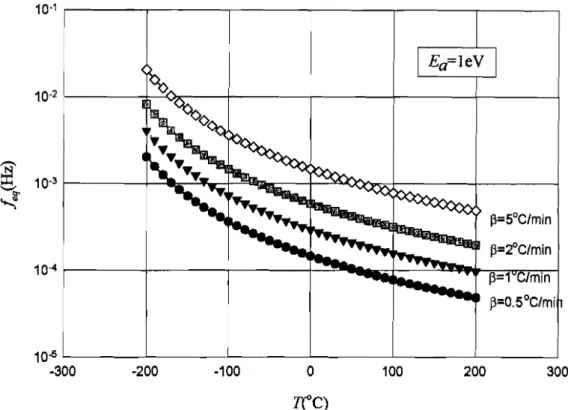
Figure 4.10 - Variation of equivalent frequency with temperature for different heating rates. ...81 Figure 4.11 - Variation of equivalent frequency with temperature for different activation

energies. . 81

Figure 4.12 - Dielectric isochronal data for different forms of polyethylene [Hedvig77) 83 Figure 4.13 - Comparing TSDC, dielectric e mechanical spectra of low density polyethylene

[Hedvig77] 83

Figure 4.14 - Propagation of a smooth twist along the chain [Boyd85b). The chain will end in

crystallographic register by a c/2 advance 85

Chapter 5

Figure 5.1 - Optical microscope photograph of methylene blue dyed vented trees (laboratory

aged in a plane-plane geometry) 88

Figure 5.2 -Water tree structure (a) oxidation dominated - field aged cables; (b) diffusion

dominated - needle test [Ross98) 100

Figure 5.3 - Electrical tree grown in an XLPE cable during testing under DC voltage

[Dissad092) 103

Figure 5.4 - Breakdown channel and water tree (wet, not dyed). It is visible the damage caused in the polymer by the breakdown. Interesting it was also the presence of the water tree (possibly the water tree has acted as an initiation for an electrical tree that end up

originating a breakdown channel) 106

Chapter 6

Figure 6.1-Press with controlled temperature used in the production of the polyethylene films. ... 112 Figure 6.2- Mould used for the production of the polyethylene samples (LOPE pellets are

visible) 113

Figure 6.3 - Modified Cigre cell 113

Figure 6.4 - Schematic representation of the modified Cigrecell., 113 Figure 6.5 - Thermal bath with the ageing cells immersed 114 Figure 6.6 - Faraday cage and setup for the electrical ageing of PE. The cells immersed in the thermal bath can be seen inside the Faraday cage. On the lower part the oil transformer is

visible 115

Figure 6.7 - Surface potential measurement apparatus 116

Figure 6.8 - Experimental procedure used to analyse space charge in LOPE. The four steps are schematically represented showing electric field, temperature and current. Selective charging corresponds to isothermal charging and discharging. Partial discharge proceeds during FTSDC. Almost complete discharge is only achieved during FIDC (schematics

adapted from [Lan~a02]) 119

Figure 6.9 - Schematic representation of the experimental setup for isothermal charge, discharge current and non-isothermal discharge current measurements 120 Figure 6.10 - Water tree grown (bush-like) in LOPE aged at 50 Hz (Leicester set). Photograph showing a water tree growing along the electric field direction, II(courtesy of

Houlgreave and co-workers) 126

Figure 6.11 - Water tree grown (viscous finger) in LOPE aged at 1.16 kHz (Leicester set). Photograph showing a water tree growing along the electric field direction, II, or perpendicular to the films surface (courtesy of Houlgreave and co-workers) 127 Figure 6.12 - Water tree grown in disc shaped LOPE aged at 50 Hz. Photograph showing a water tree growing perpendicularly to the electric field direction, .L,or parallel to the disc

surface (courtesy of Houlgreave and co-workers, ) 128

XVll

threshold level as the minimum in (a). The fractal dimension of the three-dimensional water tree is calculated asDcal+l (see Equation 6.1) 131

Chapter'

Figure 7.1 - Optical microphotography obtained under reflectance polarised light of a microtomed unaged LDPE sample (sample thickness == 1 mm) 135 Figure 7.2 - Optical microphotography obtained under reflectance polarised light of the same microtomed sample as in Figure 7.1 at a higher magnification 136 Figure 7.3 - SEM microphotographs of unaged LDPE. The images are x 5000 (a) and x 1000

(b) magnified 137

Figure 7.4 - AFM images of the surface of unaged LDPE. Microphotographs (a) and (b) were taken with different magnifications along the depth of the two opposite surfaces of the

disc shaped samples are observed 138

Figure 7.5 - AFM photographs of the same region of an unaged LDPE disc sample. The area marked as a square in part (a) is that observed at the higher magnification in part (b) 139 Figure 7.6 - Three-dimensional plot of the photograph in Figure 7.5 - (b) 140 Figure 7.7 - DSC spectra for unaged LDPE; heating/cooling rate of 1°C/min (a) and of 5°C/min (b). The arrows show the direction of temperature change, so that the upper curve corresponds to sample cooling and the lower one to sample heating 141 Figure 7.8 - Three-dimensional plot showing the surface potential of an unaged LDPE sample

after hot pressing (no further treatment) 143

Figure 7.9 - Decay of the surface potential in the same sample as shown in previous figure. ... 143 Figure 7.10 - X-ray difraction spectrum for an unaged sample of LDPE. 144 Figure 7.11 - Typical charge and discharge current curves for a LDPE sample (thermally aged sample at 40°C for 1500 h in 1M NaCI- Charging conditions: 2 kV/mm, 27 h, 30°C)... ...156 Figure 7.12 - Dielectric spectra at 30°C of LOPE for samples electrically aged (AC, 6 kV/mm, 50 Hz, 1M NaCI solution) for 1500 h at different temperatures 157 Figure 7.13 - Dielectric spectra at 30°C of LDPE for samples electrically aged (AC, 6 kV/mm, 50 Hz, 1M NaCI solution) at 40°C for different ageing times 158 Figure 7.14 - Dielectric spectra at 30 °C of LDPE for samples thermally aged (no AC, 1M

Figure 7.15 Dielectric spectra at 30°C of LDPE for samples aged electrically (AC-6 kV/mm, 50 Hz) and thermally (no AC) at 40°C in a 1M solution of NaCI for different ageing time. ... 160 Figure 7.16 - Dielectric spectrum at 30°C of LDPE unaged sample 161 Figure 7.17 - Dielectric spectrum at 30°C of LDPE of an electrically aged sample (AC, 6

kV/mm, 50 Hz, 1500 h, RT, 1M NaCI) 162

Figure 7.18 - Dielectric spectrum at 30°C of LDPE of an electrically aged sample (AC, 6

kV/mm, 50 Hz, 1500 h, 35°C, 1M NaCl) 163

Figure 7.19 - Dielectric spectrum at 30°C of LDPE of an electrically aged sample (AC, 6

kV/mm, 50 Hz, 1500 h, 40°C, 1M NaCl) 164

Figure 7.20 - Dielectric spectrum at 30°C of LDPE of an electrically aged sample (AC, 6

kV/mm, 50 Hz, 1000 h, 40°C, 1M NaCl) 165

Figure 7.21 - Dielectric spectrum at 30°C of LDPE of an electrically aged sample (AC, 6

kV/mm, 50 Hz, 500 h, 40°C, 1M NaCI) 166

Figure 7.22 - Dielectric spectrum at 30°C ofLDPE of a thermally aged sample (no AC, 1500

h, 40°C, 1M NaCI) 167

Figure 7.23 - Dielectric spectrum at 30°C of LDPE of a thermally aged sample (no AC, 1000

h, 40°C, 1M NaCI) 168

Figure 7.24 - Dielectric spectrum at 30°C of LDPE of a thermally aged sample (no AC, 500

h, 40°C, 1M NaG) 169

Figure 7.25 - Cole-Cole plot for unaged LDPE (for the LF region) 170 Figure 7.26- Cole-Cole plot for electrically aged LDPE (only for the LF region), 6kV/mm,

50Hz, 1500h, 40°C, 1M NaCl. 170

Figure 7.27 - Equivalent circuits for (a) unaged sample and electrically aged sample 6kV/mm, 50Hz, 1500h, 40°C, 1M NaCI: (b) with two low frequency peaks and (c) with a low

frequency peak and DC conductivity 171

Figure 7.28- ICC and IDC results for the same run (thermally aged sample at 40°C in 1M NaCI for 1500 h and charging/discharging conditions are:T,» 30°C,E=2 kV/mm andtc

/ t«

=

Ih/2h) 172

Figure 7.29 - FfSDC for two different runs in the same thermally aged LDPE sample with the same charging/discharging conditions(Tj=30°C,E

=

2 kV/mm, tc/td= Ih/Zh)... 175

xix

Figure 7.31 - LDPE thermally aged sample results for different charging fields (charging/discharging conditions: T;=30°C, tc/td=1h/2h and E

=

1,2,3,4& 5 kV/mm).

(a) ICC; (b) IDC; (c) FfSDC and (d) FIDC 176

Figure 7.32 - FfSDC plot showingj/E (same conditions as in Figure 7.31). The presence of a

threshold at 3 kV/mm is visible 176

Figure 7.33 _ LDPE thermally aged sample results for different charge/discharge times' ratios (charging/discharging conditions: T;=30°C,E=2 kV/mm, tJtd= 1h/2h, 3h/3h, 1h/21h&

1h/2h). (a) ICC; (b) IDC; (c) FTSDC and (d) FIDC 177

Figure 7.34 - LDPE thermally aged sample results for different charging fields (charging/discharging conditions: T;==2°C,tJtd=1h/2h and, E=2& 4 kV/mm). (a) ICC;

(b) IDC; (c) FfSDC and (d) FIDC 178

Figure 7.35 - FfSDC plot showingj/E (same conditions as in Figure 7.34) 178 Figure 7.36 - FfSDC spectra of a LDPE thermally aged sample results for different charge/discharge times' ratios (charging/discharging conditions: T;=30°C, E=2 kV/mm,

tJtd= 1h/2h& 1h/3h) 179

Figure 7.37 - Comparing charge and discharge currents for thermally aged (in 1M NaCl solution at 40°C for 1500h) and unaged LDPE withT;=30°C,E=2 kV/mm 180 Figure 7.38 - Comparing final discharge currents for thermally aged (in 1 M NaCl solution at 40°C for 1500h) and unaged LDPE withTj=30°C,E=2 kV/mm 181

Figure 7.39 - LDPE electrically aged sample results for different charging fields (charging/discharging conditions: Tj=2°C, tJtF1h/2h and, E=2, 3 & 4 kV/mm). (i) and

(ii) are runs made under the same conditions but run 3 (i) - was one of the first runs made while run 30(ii) - was one of the last ones. (a) ICC; (b) IDC; (c)FTSDCand (d) FIDe.

... 194 Figure 7.40 -FfSDC plot showingj/E (same conditions as in Figure 7.39) 194 Figure 7.41 - FTSDCfor two different runs in the same electrically aged LDPE sample with the same conditions (T;= 2°C,E =2 kV/mm,tJtd= 1h/2h - corresponding to run 3 (i) and run 30(ii) in Figure 7.39). (a) ICC & IDC and (b) FfSDC 195 Figure 7.42 - FTSDC spectra of a LDPE electrically aged sample results for different charge/discharge times' ratios (conditions:T,» 2°C, E=3 kV/mm, tcltd== 1h/1h, 1h/2h&

1h/4h) 195

Figure 7.44 - Space charge profile of an unaged LDPE sample (measurement conditions: +2.5 kVoc. pulse +400V, 5 ns, immediately after DC voltage application (a) and 2h later (b) .

... 200 Figure 7.45 - Space charge profile of thermally aged LDPE sample (thermal ageing conditions: 50°C in 1 M NaCl for 1500 h; measurement conditions: +2.5 kVoc, pulse +400V, 5 ns, immediately after DC voltage application (a) and 2h later (b) 201 Figure 7.46 - Space charge profile of a dried (in air at RT) water treed LDPE sample (electrical ageing conditions: 6 kV/mm, 50 Hz at 50°C in 1 M NaCl for 1500 h; measurement conditions: +2.5 kVoc. pulse +400V, 5 ns, immediately after DC voltage

application (a) and 2h later (b) 201

Figure 7.47 - Space charge profile of a water treed LDPE sample after immersion in distilled water for approximately 24h (electrical ageing conditions: 6 kV/mm,50 Hz at 50°C in 1 M NaCI for 1500 h; measurement conditions: +2.5 kVoc, pulse +400V, 5 ns, immediately after DC voltage application (a), lh after (b) and 2h after (c) 203 Figure 7.48 - Water trees in a methylene blue dyed LDPE sample (parallel to the film surface). Ring formation results from the presence of air bubbles on the sample surface during ageing (water trees grow at this new interface were the local field is higher)... 204 Figure 7.49 -Details of water trees (perpendicular to the film surface) in a microtomed aged LDPE sample of thickness 1 mm (the water trees are methylene blue dyed and the dark

lines are the sample surface) 205

Figure 7.50 - Water tree grown in disc shaped LDPE aged at 1 kHz (Lisbon set). Photograph shows a water tree growing perpendicular to the electric field direction, ..1. 205 Figure 7.51 - LDPE and XLPE spectra (main difference the band of acetophenone at 1720

em") 212

Figure 7.52 - LDPE spectra of water treed region in electrically aged (6 kV/mm, 50 Hz, 1M NaCl, RT, 500h) and unaged samples in the wave number region [1500, 1900J em".... 213 Figure 7.53 - LDPE spectra of unaged and thermally aged in 1M NaCl aqueous solution

samples 213

xxi

Figure 7.57 - Weibull probability plot of the breakdown times for samples aged at 40°C. The

full line is the fit using the White technique 219

Figure 7.58 - Weibull probability plot of the breakdown times for samples aged at 50°C. Shown is the fit using the White technique (full line) 219

AppendixB

Figure B.1 - A coastline is a self-similar fractal object. In the figure is an example, part of the coastline of the Norway [Feder88]. The number of squares and therefore the value of the

List of tables

Chapter 2

Table 2.1 -Bond parameters [Rosen93] .., , 11

Table 2.2 - Relaxation peaks notation [partially from Boyd85a] 15 Table 2.3 - Some properties of different forms of polyethylene 19 Table 2.4 - XLPE void characteristics for different curing methods [Steennis90] 21 Table 2.5 - Activation energies (kcallmol) after [McCrum67] 23

Chapter 3

Table 3.1- Binding energies for some covalent bonds common in polymers [Dissado92]....28 Table 3.2 - Comparison between ionic and electronic conduction (based on a table presented

by Ieda [Ieda84]) 32

Table 3.3 - Transient currents behaviour with different experimental parameters (adapted

from [Das Gupta76,97] & [Wintle83]) .40

Chapter 4

Table 4.1 - Some empirical and physical models for dielectric relaxation [Jonscher83],

[Scarpa95], [Havriliak97] and [Das Gupta99]. 55

Table 4.2 - Summary of the main types of dielectric response found in materials 63 Table 4.3 - Power-law response from Weron's probabilistic model [Weron93]. 79 Table 4.4 - Special cases of empirical functions [Weron93] 80 Table 4.5 - Dielectric loss peaks temperature (K)from litterature for oxidised LDPE 84 Table 4.6 - Activation energies for the dielectric loss peaks of PE from dielectric data 85

ChapterS

Table 5.1 - Literature survey of FfIR results found in electrical ageing studies of polyethylene (mainly low-density and crosslinked polyethylene) 94 Table 5.2 - Distribution of the more important products according to the oxidation conditions

[Xu94] 96

Chapter 6

Table 6.1 - Measurement history of thermally aged LDPE sample at 40°C during 1500 h in

1M NaCl. 122

Table 6.2 - Measurement history of an unaged sample 123

Table 6.3 - Measurement history of a sample aged at 40°C, 1500 h, 1M NaC!, AC 6kV/mm,

xxiv

Chapter 7

Table 7.1 - Results for the two main diffraction peaks (110) and (200), crystallinity content and crystallite size for LDPE (three different samples: labelled LDPE a, b and c) and

XLPE (two different samples: labelled XLPEaandb) 145

Table 7.2 - Relation between TSDC peaks and the frequency of the loss peaks 148 Table 7.3 - Possible frequency intervals for the position of dipolar loss peaks of LOPE in an

isochronal plot at 30°C 148

Table 7.4 - Fittting results for the dielectric spectra of LOPE samples (unaged and AC aged). ... 155 Table 7.5 - Thermally aged LDPE relaxation times, total charge, charge centroid, mobility and activation energy for the broad peak in FTSDC by the initial rise method calculated from the same data as in Figure 7.30. (change with the charging/discharging temperature

for a charging field of 2kV/mm) 187

Table 7.6 - Thermally aged LDPE relaxation times, total charge, charge centroid, mobility and activation energy for the broad peak in FTSDC by the initial rise method calculated from the same data as in Figure 7.34 (change with the charging field for a

charging/discharging temperature of 30°C) 188

Table 7.7 - Thermally aged LOPE relaxation times, total charge, charge centroid, mobility and activation energy for the broad peak in FTSDC by the initial rise method calculated from the same data as in Figure 7.34 (change withtltdfor a charging field of2kV/mmat

a charging/dicharging temperature of 30°C) 189

Table 7.8 - Thermally aged LDPE relaxation times, total charge, charge centroid, mobility and activation energy for the broad peak in FTSDC by the initial rise method calculated from the same data as Figure 7.34 (change with the charging field for a

charging/discharging temperature of 2°C) 190

Table 7.9 - Peak decomposition of the broad FTSDC peak situated at 50°C to 60 °C for some selected runs presented previously for the thermally aged polyethylene 191 Table 7.10 - Electrically aged LDPE relaxation times, total charge, charge centroid, mobility and activation energy for the broad peak in FTSOC by the initial rise method calculated from the same data as Figure 7.37 (change with the charging field for a

charging/discharging temperature of 2°C) 198

Table 7.12 - Results for the estimation of multifractal dimensions (Leicester samples)

(solution 0.05M NaCI at (31±4)OC) 207

Table 7.13 - Results for the fractal dimension of water trees grown in LDPE (Lisbon Samplesr' (Frequency 1.0 kHz; solution O.IM (NaCl) at (50±2) °C) 207

Table 7.14 - SEM Images (3D analysis) 208

Table 7.15 - Estimated parameters (shape and characteristic time) obtained using the White method [White69, Montanari98] for the different ageing temperatures (also the % of

censored data is shown) 217

Table 7.16 - Time (h) at which a given percentage of samples will have failed (calculated

List of symbols and most commonly used acronyms

AC- alternating current

AFM- atomic force spectroscopy C - capacitance

Co- geometric capacitance

D -dielectric displacement or dielectric induction

DC- direct current

Deal- calculated fractal dimension (similarity)

D_{f -} diffusion coefficient

Dq- generalised fractal dimension (of order q)

Dwr- water tree estimated fractal dimension (capacity)

Deal-calculated value of the fractal dimension of a water tree image

DRS- dielectric relaxation spectroscopy

DSC- differential scanning calorimetry

E- electric field

Ea- activation energy

Ee- conduction band energy level Ee- electron energy

Er

-

Fermi energy level Eg- band gap energy EL-local electric field

E;- valence band energy level

ESCA- electron spectroscopy for chemical analysis G - conductance

F- free energy

FD- frequency domain

FIDC- final isothermal discharging current

FTIR- Fourier transform infrared red spectroscopy

FTSDC- final thermally stimulated discharging current

G -conductance

HDPE- high density polyethylene

I -

current

IC- inter-cluster exchanges

ICC- isothermal charging current

IDC- isothermal discharging current

HF- high frequency

L- water tree length

f - water tree length

WPE-low density polyethylene IF- low frequency

LFD- low frequency dispersion

MDPE- medium density polyethyelene

MF- medium frequency

Mn - number-average molecular weight M w - weight-average molecular weight

MWS- Maxwell-Wagner-Sillars

No- Avogadro's number

Nd ,....number of permanent dipoles

P- polarization

P_F

(t)

-

cumulative distribution function (probability of failure)

PD - partial discharges

PE- polyethylene

Q-charge

Qc- charge accumulated during ICC

Qd- charge released during total discharge

QFIDC- charge released during FIDC

QFTSDC- charge released during FTSDC

QICC- charge accumulated during ICC QIDC- charge released during IDC

QDC- quasi-DC

R- resistance

RT- room temperature S- entropy

SALS small angle light scattering

XXiX

S(L)

-

total damage in a water tree

SEM- scanning electronic microscopy

SeLe

-

space charge limited current

T- temperature

T,- charging temperature in isothermal current measurements and initial temperature in thermally stimulated measurements

TD- time domain

TFL- trap filled limit

Tg- glass transition temperature

Tm- melting transition temperature

T1NlX- maximum peak temperature for thermally stimulated measurements

TSe

-

thermally stimulated charging current

TSDe- thermally stimulated discharging current

U- internal energy

V- applied voltage VTFL- trapped filled limit

VIr- transition voltage between ohmic and space charge limited conduction

XLPE- crosslinked polyethylene

WLF- Williams-Landel-Ferry Z - impedance

a - shape parameter in Weibull statistics or

distance between neighbouring potential wells

d- sample thickness

d_{f -} fractal dimension

d,- fractal dimension of a water tree

e- electron charge

f

-

frequency

g(t)

-

probability density function

h- Planck's constant

1i

=

h/2n

j -

current density

ke

-Boltzmann constant

m;

-

electron's effective mass

n- carrier concentration

n,- number of traps

p-pressure q-charge

t-time

tanS-dielectric loss

x-position

cP - dielectric response function or dielectric decay function

lJ' - dielectric relaxation function or potential decay function ex - polarisability

P

-

heating rate or

width at half height of a peak

PPF

-

Poole-Frenkel coefficient

X- susceptibility

Xs

-

static susceptibility

S

-

angle between the electric field and the polarization

S(x)

-

delta function

Er:dielectric constant or relative permittivity (sometimes also representedbye)

eo

-

permittivity of vacuum

e;

-

static permittivity (occurs at long time or low frequency)

e;- high frequency permittivity (occurs at short time and high frequency)

Crs- static dielectric constant (occurs at long time or low frequency)

e.;

-

high frequency dielectric constant (occurs at short time and high frequency)

4' -

work function

f/>m - metal work function

A

-

wavelength

AD- Debye screening length

xxxi

/Jd- dipole moment

V- frequency

e

-

Bragg angle for X-ray diffraction or

ratio of number of electrons in conudction band to the number of traps

p- resistivity or

Pm-density

U- conductivity

Us- surface conductivity

ca

-

angular frequency (sometimes also simply called frequency, however its relation to

f

is

W=21if)

'r - relaxation time

'r_eq- equivalent relaxation time for T_min thermally stimulated measurements

"(... )science does not progress tidily"

E. Mendonza in History ofphysics

The word insulator comes from the latin "insula"

suggesting thatitis isolated from its surroundings(... )

L.A. Dissado &

J.e.

Fothergill

According to the above statement a perfect insulator will be electrically completely isolated whatever is contained inside it, allowing no current to flow. Yet the perfect insulator does not exist and the work developed here studies a tiny part of the departures from perfection of one of the best insulating polymers (also the chemically most simple known): polyethylene.

For decades insulating polymers have been widely used in power cables. Initially low density polyethylene (LDPE) and later crosslinked polyethylene (XLPE) have been the most common insulators in medium and high voltage power cables. Electrical ageing of the insulation is inevitable and may in the long run give rise to costly cable failure. Understanding the ageing related phenomena is essential to achieve better quality materials that will provide a extended life time of the cables.

This work is an attempt to regard ageing from two different points of view: the local damage (represented by water treeing and breakdown channels) and the bulk ageing (represented by a change in bulk dielectric and electrical properties). Localised damaged is accessed by means of fast Fourier infrared spectroscopy (FfIR), breakdown statistics, fractal analysis of water trees, etc. The bulk ageing was studied either by dielectric relaxation spectroscopy (DRS), thermally stimulated discharge currents (TSDC) or pulsed electroacoustic (PEA)), etc. The task of relating these two aspects is a difficult one and can only be achieved for longer ageing times since initial ageing is dominated by breakdown from manufacture and processing defects and contaminants.

2 Electrical ageing studies of polymeric insulation for power cables

and mechanical stresses that end up resulting in a permanent degradation of the material even if not leading directly to dielectric breakdown. Thus electric and dielectric bulk properties will change during ageing. Pre-existing traps and/or new traps will be filled with space charge that was able to diffuse in and properties such as dielectric constant and conductivity are liable to be affected.

One of the most puzzling phenomena in electrical ageing is water treeing (localised damage).

Itis the result of the degradation of the polymer under the effect of an alternate electric field and aqueous salts [Steennis90, Dissadovz, Ross98, Crine98]. Since the first time it was detected nearly three decades ago, much work has been published showing that many different factors seem to affect water tree inception and growth, such as: temperature, mechanical stress, type and concentration of ionic salts, applied electric field (frequency and magnitude), polymer morphology and composition, etc. Revealing the complex nature of water tree mechanisms of inception and growth, conflicting and difficult to reproduce results have been reported either for field aged or laboratory accelerated aged specimens. This shows the importance of a good characterisation of sample properties prior to and after ageing. Many experimental techniques have been used: dielectric relaxation spectroscopy analysis (DRS) [Scarpa95, Das Gupta99], thermally stimulated depolarisation currents (TSDC) [Bamji93], laser intensity modulation method (LIMM) [Wilbbenhorst98], pulsed electroacoustic spectroscopy (PEA) [Ohki98], differential scanning calorimetry (DSC), Fourier transform infrared spectroscopy (FfIR), depolarisation currents, etc. Many theoretical models have been proposed but none seems to fully explain inception and growth mechanisms. Over the last few years some progress has been made into finding a suitable theoretical model [Zeller8?&91, Ross92&98, Xu94]. The experimental results and models point to a complex mechanism involving electro, mechano and chemical processes. In the laboratory special accelerated ageing techniques were developed. Nevertheless when comparing field and laboratory aged specimens the dominant mechanism in the later seems to be electro-mechanical while in the former the electro-chemical seems to dominate. In order to obtain better quantitative data, different characterisation methods must be used and also it is necessary to gather information from different experimental techniques.

common insulators is by no means without controversy, quoting Shaw and Shaw [Shaw84]: "From a material-science viewpoint the common use of polyethylene as an experimental

treeing substrate material have been a disastrous mistake. (... ) Crosslinked or not, the

chemical and physical state of polyethylene is perhaps the more dependent on past history

(... ) than any other common polymer. Polyethylene not only has a multitude of chemical

variations (... )but a large portofolio of crystalline habits, organisation and orientation.(... )

the modulus of polyethylene can be made to vary experimentally over two orders of

magnitude by control of the orientation and crystallinity alone". The previous sentence reveals some of the difficulties found in studying the effect of ageing on this polymer. In order to overcome this a new experimental procedure proposed by Neagu [NeaguOl] for high insulating polymers was used for the first time in the study of transport and trapping of charge in polyethylene. This procedure combines usual isothermal measurements of charge and discharge currents and non-isothermal measurements (called final thermally stimulated discharge currents - FTSDC).Also takes in account the residual charge that remains trapped at the end of the isothermal step by including a final discharge (FIDC) step that discharges completely the sample before the next run takes place.

The thesis is divided into two different parts. In the first part we have tried to give the reader a general view of the state of the art that however does not intend to be a complete description of all available information.

Chapter 2 is a brief review of polymer characteristics and properties focusing on polyethylene. Polymers are classified according to different features such as: origin, response to temperature (thermoplastic and thermoset polymer, chemistry of synthesis and structure). Still related with the polymeric structure are the bonds, morphology and crystallinity (amorphous and semi-crystalline polymers) that are briefly described. The mechanical properties and relaxation processes are also discussed. In the final part of the chapter specific polyethylene characteristics are presented.

4 Electrical ageing studies of polymeric insulation for power cables

For Chapter 4 the problem of dielectric relaxation is dealt in particularly with application to polyethylene. The dielectric response is presented in the time and frequency domains. Empirical models starting with Debye model are treated. The effect of temperature on the dielectric relaxation spectra is focused and the importance of dielectric data presentation in order to identify mechanism is reviewed. The main classes of dielectric solid materials according to their dielectric response are presented. Next physical models to explain the different observed behaviour are dealt with (especially Jonschers universal law and Dissado-Hill cluster model). The relation between data from non-isothermal currents (TSDC) and dielectric relaxation spectrum is made. Finally published results of dielectric relaxation spectra of polyethylene are discussed.

As for Chapter 5 electrical ageing is presented with main attention on water treeing and a brief review on electrical treeing and dielectric breakdown. A space charge model for electrothermal ageing that allows lifetime estimation is presented.

The second part of this thesis begins with Chapter 6 and 7 where the experimental procedures followed and the results obtained during this research are presented.

Sample preparation and ageing and the different techniques used to characterise the unaged and (electrical and thermally) aged specimens are described in Chapter 6. Preparation of samples was made from pellets by hot pressing and disc-shaped specimens were obtained. These samples were submitted to different ageing conditions being always under planar electrode geometry where the electrodes were the solution of NaCl. Samples suffered electrical plus thermal ageing (also called AC or electrical ageing) at different temperatures and for different time periods (the applied AC field was mainly at 50 Hz with an amplitude of

6 kV/mm)or just thermal ageing (also called no-AC or thermal ageing)

In Chapter 7 the results of the measurements made are presented and discussed. The characterisation of unaged samples was made using microscopy (optical, SEM, AFM), DSC, surface potential measurements and X-ray diffraction. Comparison between unaged and aged samples (AC and no-AC ageing) was made by dielectric relaxation spectroscopy in the frequency range of 10-5Hz to 105Hz. To cover this broad range three different measurements techniques were used: in the low frequency range (LF) - 10-5Hz to 10-1Hz - time domain measurements were performed; for the medium frequency range (MF) - 10-1Hz to 102Hz -measurements were performed using a lock-in amplifier and in the high frequency range (HF)

distinguish some differences between electrical plus thermal ageing and just thermal ageing since unaged samples were difficult to analyse. The PEA technique helped to obtained the space charge profile of the samples (unaged, AC and no-AC aged samples). Some of the samples showing water trees were dyed with methylene blue and used (together with some other samples from other authors) to estimate the fractal dimension of water trees. The chemical changes were studied by FTIR and some evidence of oxidation was found for aged samples. A breakdown statistics using the two-parameter Weibull function was made.

Chapter 2. Polyethylene: polymer properties

Polymer: from the Greek "many-membered"

In this chapter a brief review of polymer characteristics is presented. Special emphasis will be given to an electrical insulator polymeric material named polyethylene (PE) that also has many other applications. Electrical and dielectric properties will be discussed in greater detail in subsequent chapters.

2.1

Polymers

In the 1920s H. Staudinger' proposed the "macromolecular hypothesis" giving rise to one of the most important type of materials now used in everyday life and also in industry.

Strictly speaking, a polymer is any large molecule (long chain macromolecule) composed of any number of smaller units (the "mers"or monomers). According to this definition any ionic crystal, such as NaCl, could be a polymer. Yet this name is restricted to materials where monomers are linked by covalent bonds. A few examples of this kind of bonds are [Rosen93]:

I I I

-C- N -0-

ci-

F- H-

-si-I / \ I

(see also Table 3.1).

The name of the polymer is usually the name of the composing monomer plus the prefixpoly.

Polyethylene is the polymer resulting from the monomer ethylene (polyethene is the leI trade name for PE):

H H

I

,

C=C

!

I

H H

i

H

H1

I

I

C-C

~ ~

"

ethylene polyethylene

The long chain structure of the macromolecules gives the polymers distinct and variable properties. The degree of polymerisation, n (also called chain length and representing the number of units in the macromolecule), is in the range 103_105 granting also high average molecular weight. In a polymer there is a distribution of molecular weights and only an average molecular weight can be define, for instance the number-average molecular weight is:

and the weight-average molecular weight is:

- LwxMx

Mw

=

~

,

L.JWx

(2.1)

(2.2)

n;

is the number of moles of the

x-mer

with molecular weight Mx , W_x

=

nxMx is the total weight of the x-mer and N

=

Ln_xthe total number of moles in the sample.

The length of the main chain can exceed 1 JAm. Flexibility and interaction of the chains together with polar group interactions (dipoles) define the mechanical and electrical properties of polymers. Many physical properties show a change at a critical (average weight) number of chain atoms around 1000. Practically all polymers are good electrical insulators/ because they have large band gaps (see 3.2), low dielectric constant and dielectric loss in a wide range of frequencies (see 4.8). Combining the good insulator characteristics and mechanical properties, polymers are ideal to be used as insulating material in electrical appliances, such as power cables.

2.1.1 Types of polymers

Polymers can be classified according to different criteria and a brief summary is given.

a) Origin

Natural - some polymers are produced by nature, examples are natural rubber, nucleic acids

and cellulose.

Natural modified - natural polymers that have been modified in order to improve their

properties for human use, such as vulcanised rubber and derived cellulose.

Synthetic- Completely artificially produced, one of the simplest is polyethylene.

b) Response to temperature

Thermoplastics - Some polymers soften when heated. If a mechanical stress is applied they

will flow. After cooling their characteristics are reversibly recovered.

Thermosets - These polymers become soft on heating. However when cooled the process is

not reversible and the initial characteristics are not recovered.

2 Conducting polymers are a more recent field of application for polymers. They are specially developed to

Polyethylene: polymer properties 9

c) Chemistry of synthesis

Addition or chain reaction- In addition polymerisation the monomer molecules are added to

the polymer chains. The unit molecule is not broken and the polymer has the same chemical formula as the monomer. The reaction involves the opening of a double bond.

Vinyl monomers (where C=C is present) produce vinyl polymers by addition reaction. Polyethylene (also a hydrocarbon polymer since it is made only of C and H atoms) is one of such kind:

Other vinyl monomers are propylene and vinyl chloride which give rise to polypropylene and poly(vinyl chloride), respectively.

Polyether is another polymer formed by addition but this time from an opening-ring reaction. The ethylene oxide ring opens to originate polyether, which contains carbon and oxygen atoms in its backbone.

Condensation or step reaction - Polymers are formed from an organic condensation reaction

where a small molecule (usually water) is also produced. Intervening monomers are multifunctional (have more than one reactive group per molecule). Polyester and polyamide (nylon-6,6) are polymers obtained in such a way.

d) Structure

Linear - The chain molecules are strictly linear. High density polyethylene (HDPE) is a

polymer prepared specially to have almost linear chains (1 to 5 CH3 branches per 1000 carbon atoms).

Branched - Main chains exhibit ramifications that can appear during polymerisation. In

polyethylene branching can occur when a hydrogen atom from a monomer or from a polymer molecule is transferred to a growing chain radical. Vinyl polymers in general contain one branch for every 104 monomer units in the chain (they are essentially linear). Low-density polyethylene (LDPE) has 15 to 30 CH3 per 1000 carbon atoms. Short branches are several units long while long branches can be as long as the main chain. Branching can have a large effect on polymer properties. Itlowers density and crystallinity (compare LDPE and HDPE in Table 2.3) and increases the number of weak points in the chains.

Crosslinked- Long polymeric chains can extend until they cross with other chains. When all

large and the material is a thermoset. Some properties change, for instance, they are less crystalline and their Young modulus is proportional to the degree of crosslinking (fraction of covalent bonds that participate in crosslinking) [Dissado92].

Crosslinking can arise in two ways. One possibility is during polymer manufacture if tri- or higher order functional monomers are used. The other is by chemical reactions in existing macromolecules (curing). This can be achieved by adding a catalyst (usually a peroxide), using radiation or a chemical hardener.

For example, XLPE (cross-linked polyethylene) is obtained during extrusion of polyethylene by adding a catalyst to the initial mixture, the more often used are dicumyl peroxide (described in more detail below) and silane.

If the polymer consists of one kind of monomers they are called homopolymers. Heteropolymers can be made of more than one type of monomers. If two different monomers are present they are called copolymers (if three different monomers are present they are named terpolymers).

Copolymers are classified according to the way monomers are distributed in the chains. A copolymer with monomers A and B distributed in a random fashion along the backbone is called random copolymers.

ABAABABBBAAB

Block copolymers have continuous blocks of the same unit.

AAAABBBBBAAAABBBBBAAAA

Both examples show linear polymers, a graft copolymer has always branched chains:

B

B

B

B

B

B

B

AAAAAAAAAAAAAAAAAAAAA

B

B

B

B

2.1.2 Bonds and structure

In a polymer the atoms are kept together by different kinds of bonding. The main type is the

covalent bond(sharing of electrons between the atoms) that joins the atoms in the polymeric

Polyethylene: polymer properties 11

hydrogen bonds due to a dipolar moment between hydrogen and oxygen -also chlorine and

fluorine- atoms from different molecules;

dipole interactions arise when dipole moments appear between atoms with an unequal share

of electrons (a hydrogen bond is a stronger dipolar interaction where the dipolar moment is higher);

ionic interactions between ions and

van der Waalsresulting from temporary dipoles created by uneven distributions of charges in

non polar atoms, for instance between carbon atoms belonging to different macromolecules. In Table 2.1 [Rosen93] typical values characteristic of these bonds can be seen.

Table 2.1 -Bond parameters [Rosen93]

Bond type Interatomic distance Dissociation energy

(nm) (eV)

Primary covalent 0.1-0.2 50-200

Hydrogen bond 0.2-0.3 3-7

Dipole interaction 0.2-0.3 1.5-3

Van der Waals 0.3-0.5 0.5-2

Ionic 0.2-0.3 10-20

As concerns the spatial arrangement one should distinguish between configurations (only by bond breaking it is possible to change the configuration) and conformation (different conformations correspond to rotation of atoms around single bonds). The geometric distribution of the atoms in the macromolecule (or any molecule) is such that it minimises the energy. In polyethylene the chain is arranged in a zigzag fashion with the carbon atoms in the backbone and the hydrogen atoms on either side corresponding to a trans conformation. In other vinyl polymers with more than one kind of different substituent groups attached to the backbone the spatial arrangement can be classified according to the way these groups are distributed (tacticity or stereoregularity). There are different stereoisomers: isotatic (identical atoms or groups are on the some side of the chain); syndiotactic (different atoms or groups alternate along the plane of the chain) and atatic (if the different atoms or groups are randomly distributed). Stereoregularity tends to increase crystallinity.

2.1.3 Morphology and crystallinity

form crystals. Linear molecules are much easier to align and arrange spatially in a regular manner. In the example referred in 2.1.2 isotactic vinyl polymers are more likely to be crystalline than atactic polymers. Branching and crosslinking are also factors that decrease crystallinity. Long side groups appearing on the backbone make the packing of the macromolecules more difficult. Also the intermolecular forces have to be strong enough to overcome thermal disorder. There are completely amorphous polymers but a completely crystalline one has never been produced. In wholly amorphous polymers the chains are arranged in a random manner presenting a "ball-like" shape. As a material in the glass phase they look transparent. A fully crystalline polymer is much more difficult to obtain but nowadays polymers with almost 100% crystallinity have been made". Ifit existed it would look completely opaque. The majority of polymers are semicrystalline and usually look milky. The polymer is composed of small crystalline regions (crystallites) and amorphous regions.

Crystalline regions may be formed from sheets, long fibres or superstructures. A first model developed was thefringed micelle model. However thermodynamically this model is unlikely to happen on a large scale. This together with new experimental evidence has led to the development of the lamellae model. Most of the polymeric materials will have crystalline regions were the long chains are folded to form sheets which are called lamellae. These look like small ribbons. Typically their dimensions are of 10

urn

wide, 1 urn long and 10 nm thick. The chains can fold and reenter the lamella in a regular or irregular (switchboard) manner or can cross from lamella to lamella or even end in the amorphous region in between (see Figure 2.1). During primary crystallisation twisted lamellae grow from nuclei in a star-like fashion forming larger structures known as spherulites (Figure 2.2). They show a Maltese cross pattern when viewed under polarised light (see photograph of PE in Figure 2.5). Usually their radius is around 10 um but can be large enough to be seen to the naked eye. They are space filling polyhedra and between the twisted lamellae there exists amorphous material and other lamellae resulting from secondary crystallisation.

3Compared with a metal were the defect concentration is on the order of ppm, it is not possible to have a totally

Polyethylene: polymer properties ₁₃

Figure 2.1 - Several lamellae showing alignment, folding and reentering of chains with the amorphous region in between [Bartnikas83].

Figure 2.2 - Spherulite grown from a nucleus with many lamellae (like a sea urchin) [Dissad092].

The degree of crystallinity (% of crystalline volume or mass present in polymer) is usually between

5-50%

[Blythe79]. It depends on thermo-mechanical history, branching and crosslinking, stereoregularity and copolymerisation.Ifa melted material is rapidly cooled or quenched it will have insufficient time to form the crystallites and will be less crystalline then a slowly cooled similar melt.Ifa polymer is stretched the chains will tend to align and the degree of crystallinity will increase.

2.3 illustrates property changes for different types of polyethylene (including degree of crystallinity).

Some experimental techniques to characterise the crystalline content of a polymer are density measurements (as stated before), infrared and Raman spectroscopy, differential scanning calorimetry (DSC), X-ray diffraction and small angle light scattering (SALS). For morphology studies several microscopy techniques have been used: optical, scanning electron microscopy (SEM), transmission electron microscopy (TEM), atomic force microscopy (AFM), etc.

2.1.4 Mechanical properties

These properties are mostly determined by density and in turn molecular length and number and length of side chains determine density. Many polymer applications use their unique mechanical properties (elasticity, viscosity, etc.). The rheological" behaviour of polymers is difficult to explain and unusual when compared with other types of materials. It is also strongly dependent on temperature and time of the applied stress. As an example, the Hooke's law of elasticity is often not verified (only for small stressesitis verified). When a yield point is reached slippage of chain results in an incomplete recovery. Finally at the ultimate stress fracture occurs. Some values for PEcan be seen in Table 2.3. Different types of rheological behaviour are:

a) Viscous flow - associated with irreversible slippage of molecular chains;

b) Rubberlike elasticity - the material shows a complete recovery after mechanical

deformation (rapid molecular movements are occurring);

c) Viscoelasticity - the material has an elastic behaviour because it is able to recover from the

mechanical deformation but it shows the deformation is dependent on the time the stress is applied so that it also shows creeps;

d) Hookean elasticity - the stress and the strain show a linear relationship (related to bond

stretching and rotation).

Polymers are viscoelastic materials.

Two simple phenomenological models have been used to explain creep and relaxation behaviour based on coupling elastic springs and viscous damping. The Maxwell model is based on springs and damping cylinders in series while the Kelvin-Voigt model uses a parallel

Polyethylene: polymer properties 15

configuration of the same elements. Molecular theories try to explain this kind of behaviour on the basis of the molecular structure of polymers.

The factors affecting mechanical properties are:

i) Interaction between the macromolecules;

ii)Flexibility of chains - with associated molecular motions (motion of branch points, rotation

of side groups, crankshaft motion, segmental motion and motion of crystallite features);

iii) Spacing ofpolar groups.

2.1.5 Relaxation processes in polymers

Besides the first order melting transition it is well know that polymers exhibit other transitions. They are usually visible both in the mechanical and the dielectric relaxation spectra of polymers (see Figure 7.7, a DSC spectrum of the LDPE samples prepared during this work). Some of the relaxations appearing in the mechanical spectra will not show up in the dielectric spectra if no dipoles are associated with that particular mechanism. Mechanisms for the same transition can be different according to their mechanical or dielectric character. For an isochronal plot (constant frequency) transitions are classified from the highest temperature to the lowest using the Greek alphabet letters ex, ~,y and S, etc. (see Figure 2.3).

InTable 2.2 a more complete labelling of the relaxation processes is presented. The polymer can show just some of these transitions and not all of them depending, for instance on the degree of crystallinity. NMR studies have also proved to be very helpful for understanding the underlying physical mechanisms causing each relaxation.

Table 2.2 - Relaxation peaks notation [adpated from Boyd85a] Number of processes Tmaxf - -(isochronal) f----Tmin

3 (semicrystalline) et(etc)

6

(ex_a) y

_S

2 (amorphous) ex(eta)

₆

y

related to thea transition (the one occurring at higher temperatures). This kind of transition is also studied by measuring the changes in some thermodynamic properties with temperature, such as density, heat capacity, etc. Density measurements have revealed that below Tg a temperature change will not change the density while aboveTgan increase in temperature will decrease the density. Below T_gthere is motion of individual atoms and small groups of atoms, no large-scale cooperative motion exist. Above Tgthe motions become of the liquid type. In low crystalline polymers (amorphous) the ex (aa) transition is well defined. This feature is typical of the glass transition, which is a cooperative phenomenon corresponding to micro-brownian motion of the chains. Itcan be associated with a kind of crankshaft motion where the tails of the chains remain in the same position. Also it was described as damped diffusion of conformational changes along the chains [Schonhals97]. It is expected that both intermolecular and intramolecular interactions will contribute. The ~ relaxation it is not yet well understood. It can be related to fluctuations of localised parts of the main chain or to rotational fluctuations of the side groups or parts of them.

p

Physical

quantity

a

.,

T,

Q

To Temperature

Figure 2.3 - Schematic diagram of phase transitions in semicrystalline polymers. Itcan be applied to both dielectric and mechanical spectra [HalI89]. For instance, P and Q can be, respectively, the real and imaginary components of the permittivity (dielectric measurements)

or of the shear compliance (mechanical measurements).

For semicrystalline polymers, according to IHedvig77] and [Boyd97] the ex transition occurs in the crystalline regions of the polymer while the ~ transition occurs in the amorphous region. Theypeak is also associated with the amorphous region and is assumed to be a kind

SThe higher temperaturea transition of sernicrystalline polymers disappears in amorphous ones. The first one