Faculdade de Ciências e Tecnologia
Departamento de Informática
Acceleration of Physics Simulation Engine through OpenCL
Dissertação para obtenção do Grau de Mestre em
Engenharia Informática
Jorge Miguel Raposeira Lagarto
Orientador:
Prof. Doutor Fernando Birra
Júri:
Presidente:
Prof. Doutor Pedro Manuel Corrêa Barahona
Arguente:Prof. Doutor João António Madeiras Pereira
Vogal:
Prof. Doutor Fernando Pedro Reino da Silva Birra
Faculdade de Ciências e Tecnologia
Departamento de Informática
Dissertação de Mestrado
Acceleration of Physics Simulation Engine through OpenCL
Jorge Miguel Raposeira Lagarto
Orientador:
Prof. Doutor Fernando Birra
Trabalho apresentado no âmbito do Mestrado em Engenharia Informática, como requisito parcial para obtenção do grau de Mestre em Engenharia Informática.
© Copyright by Jorge Miguel Raposeira Lagarto, FCT/UNL, UNL
Hoje em dia, a simulação física é um tópico relevante em vários domínios, desde áreas científi-cas como a medicina, até ao entretenimento como efeitos em filmes, animação de computador e jogos.
Para facilitar a produção de simulações mais rápidas, os programadores usam motores de física, pois eles oferecem uma grande variedade de funcionalidades como simulação de corpos rígidos e deformáveis, dinâmica de fluídos ou detecção de colisões. As indústrias do cinema e dos jogos de computador usam cada vez mais os motores de física para introduzir realismo nos seus produtos. Nestas áreas, a velocidade é mais importante do que a precisão e têm sido desenvolvidos esforços para atingir simulações com alta performance. Além de algoritmos de simulação física mais rápidos, o avanço na performance das Unidades de Processamento Grá-fico (GPUs) nos últimos anos tem levado os programadores a transferir cálculos pesados para este tipo de dispositivos, em vez de os realizar na Unidade Central de Processamento (CPU). Alguns motores de física já fornecem implementações em GPU de algumas funcionalidades, nomeadamente na detecção de colisões entre corpos rígidos.
Neste trabalho pretendemos acelerar uma funcionalidade presente na grande parte dos mo-tores de física: a simulação de tecidos. Como a detecção de colisões é um dos maiores facmo-tores que limitam a eficiência neste tipo de simulação, vamo-nos concentrar especificamente em mel-horar esta fase. Para atingir uma aceleração considerável, planeamos explorar o incrível par-alelismo do GPU através do desenho de algoritmos eficientes na arquitecturaOpen Computing Language(OpenCL). Finalmente, irá ser elaborado um estudo para comparar a performance de uma implementação sequencial em CPU com a solução paralela apresentada em GPU.
Palavras-chave: Motor de física; Simulação de tecidos; Detecção de colisões; GPU - Unidade de Processamento Gráfico; OpenCL - Open Computing Language; BV - Volume envolvente; BVH - Hierarquia de volumes envolventes
Nowadays, physics simulation is a relevant topic in several domains, from scientific areas like medicine to entertainment purposes such as movie’s effects, computer animation and games.
To make easier the production of faster simulations, developers are using physics engines because they provide a variety of features like rigid and deformable body simulation, fluids dynamics and collision detection. Computer game and film industries use increasingly more physics engines in order to introduce realism in their products. In these areas, speed is more important than accuracy and efforts have been made to achieve high performance simulations. Besides faster physical simulation algorithms, GPUs’ performance improvement in the past few years have lead developers to transfers heavy calculation work to these devices instead of doing it in the Central Processing Unit (CPU). Some engines already provide GPU implementations of several key features, particularly on rigid body collision detection.
In this work we want to accelerate a feature present in most of the current physics engines: cloth simulation. Since collision detection is one of the major bottlenecks in this kind of simu-lation, we will focus specifically in improving this phase. To achieve a considerably speed-up we plan to exploit the massive parallelism of the Graphics Processing Unit (GPU) by design-ing an efficient algorithm usdesign-ing the Open Computdesign-ing Language (OpenCL) framework. Finally, a study will be made to compare the performance of a sequential CPU approach against the parallel GPU proposed solution.
Keywords: Physics engine; Cloth simulation; Collision detection; GPU - Graphics Processing Unit; OpenCL - Open Computing Language; BV - Bounding Volume; BVH - Bounding Vol-ume Hierarchy
Acronyms xvii
1 Introduction 1
1.1 Motivation 2
1.2 Expected contributions 2
2 State of Art 3
2.1 Physics Engines 3
2.1.1 PhysX 3
2.1.2 Havok 4
2.1.3 Bullet 4
2.1.4 GPU Acelleration in Physics Engines 4
2.2 Cloth Collision Detection 6
2.2.1 Spatial Enumeration 7
2.2.1.1 Regular Grids 7
2.2.1.2 Spatial Hashing 8
2.2.2 Bounding Volume Hierarchies 8
2.2.2.1 Bounding Volume choice 8
2.2.2.2 BVH Construction 10
2.2.2.3 BVH Traversal 10
2.2.2.4 BVH Update 11
2.2.3 GPU Implementations 12
2.3 OpenCL framework 16
3 OpenCLKernels 19
3.1 Introduction 19
3.2 Bounding Volume Hierarchy Construction 19
3.2.1 BVH Construction Kernel 19
3.2.1.1 Root Construction Kernel 19
3.2.1.2 Remaining Hierarchy Construction Kernel 21
3.2.2 BVH Construction Kernel Optimizations 23
3.2.2.1 Adaptive Work Group Size Optimization 24
3.2.2.2 Small Splits Optimization 25
3.2.2.3 Large Nodes Optimization 25
3.2.3 Compaction Kernel 28
3.2.3.1 Compaction Kernel for Small Arrays 28
3.2.3.2 Compaction Kernel for Large Arrays 29
3.3 Broadphase Collision Detection Kernel 31
3.3.1 Simple Broad Phase Collision Detection 31
3.3.2 Front-Based Broad Phase Collision Detection 35
3.4 Narrow Phase Collision Detection 37
3.5 Update Kernel 37
4 Results Analysis 39
4.1 Construction Kernels Results 39
4.1.1 Adaptive Construction Kernel Results 40
4.1.2 Small Splits Construction Kernel Results 41
4.1.3 Large Nodes Construction Kernel Results 42
4.1.4 Compaction Kernel Results 44
4.2 Broad Phase Collision Detection Kernels Results 45
4.2.1 Simple Broad Phase Collision Detection Kernel Results 45 4.2.2 Front Based Broad Phase Collision Detection Kernel Results 46
4.3 Narrow Phase Collision Detection Kernel Results 47
4.4 Update Kernel Results 47
5 Conclusions and Future Work 49
A Appendix 51
A.1 Reduction and Scan Algorithms 51
A.2 Common Functions 53
A.3 BVH Construction Kernels 61
A.3.1 BVH Root Construction Kernel 61
A.3.2 BVH Construction Kernel 62
A.3.3 Small Splits Construction Kernels 63
A.3.4 Large Nodes Construction Kernels 68
A.3.4.1 Large Nodes Construction Kernels - Get Split Point 68 A.3.4.2 Large Nodes Construction Kernels - Split By Centroid 69 A.3.4.3 Large Nodes Construction Kernels - Build k-Dops 72
A.3.5 Compaction Kernels 75
A.3.5.1 Compaction Kernel for Small Arrays 75
A.3.5.2 Compaction Kernels for Large Arrays 76
A.4 Broadphase Collision Detection Kernels 78
A.4.1 Simple Broadphase Collision Detection Kernel 78
A.4.2 Front-Based Broadphase Collision Detection Kernel 80
A.5 Narrowphase Kernel 84
2.1 Collision detection on the GPU 5
2.2 Collision types in cloth meshes 7
2.3 Bounding Volumes 9
2.4 Example of 2D Morton Code grid 13
2.5 SAH method ilustration 13
2.6 Index space orgainzation on OpenCL 17
2.7 Memory architecture in OpenCL device 17
3.1 Root construction kernel scheme 20
3.2 Build BVH Kernel Scheme 22
3.3 Construction timings per level 24
3.4 Kernels to get the split point for large nodes 26
3.5 Kernels to reorder primitives’ indices 27
3.6 Kernels to build a BV from several blocks of primitives 28
3.7 Compaction kernel scheme for small arrays 29
3.8 Compaction kernel scheme for large arrays - First Kernel 30 3.9 Compaction kernel scheme for large arrays - Second Kernel 30 3.10 Compaction kernel scheme for large arrays - Third Kernel 31 3.11 Broad phase kernel scheme: two internal nodes overlap 32 3.12 Broad phase kernel scheme: one internal node and one leaf overlap 33
3.13 Broad phase kernel scheme: two leafs overlap 34
3.14 Front decomposition 35
3.15 Front update 36
3.16 Update Kernel Scheme 38
4.1 Benchmark models 40
4.2 Adaptive Kernel timings per level 40
4.3 Small Splits Kernel timings 41
4.4 Large Nodes Kernels timings 43
4.5 Time consumed by the compaction kernel 44
4.6 Broad Phase kernel performance 45
4.7 Cloth dropping over the Bunny model 46
4.8 Broad Phase with and without the front based approach 46
4.9 Narrow Phase Kernel timings 47
4.10 Update kernel timings per level 48
4.1 GPUs specifications 39
4.2 Construction phase timings 43
4.3 Construction phase timings for two different devices 44
4.4 Update phase timings 48
AABB Axis-Aligned Bounding Box.
API Application Programming Interface.
BV Bounding Volume.
BVH Bounding Volume Hierarchy.
CCD Continuous Collision Detection.
CPU Central Processing Unit.
CUDA Compute Unified Device Architecture.
DOP Discrete Oriented Polytope.
GPU Graphics Processing Unit.
LBVH Linear Bounding Volume Hierarchy.
OBB Oriented Bounding Boxes.
OpenCL Open Computing Language.
PPU Physics Processing Unit.
SAH Surface Area Heuristic.
SM Streaming Multiprocessor.
SP Streaming Processor.
Physics is a huge area of investigation, which combined with computer science, is used to simulate aspects of the physical world. From this union results the physics engine, a software capable of performing an approximate simulation of the real world, based on physics laws. Rigid and soft body dynamics, collision detection and fluid simulation are some of the features offered by this kind of software.
Physics engines are used in a variety of domains, from scientific research to computer games or movie’s special effects. While some areas need high accuracy, which leads to expensive computations, in others speed of simulation is more important than precision. In computer game and film industries, physics engines usually resort to simplified calculations, lowering their accuracy and accelerating the simulation, providing real time gameplay and continuous animation.
To meet this demand for speed, physics engines began to explore the power of actual GPUs (Graphics Processing Unit). In the past few years, GPUs have improved their performance dramatically, when compared to CPUs. This gap does not have to do with processor’s clock speed-up, but with the difference in the number of cores between CPUs and GPUs. Such a high number of cores results on a considerable increase in the amount of work a GPU performs at once, by doing tasks in parallel. Each core can process large data sets by running thousands of threads at the same time.
To help developers take advantage of these capabilities, NVIDIA launched Compute Unified Device Architecture (CUDA) in 2007, providing an easy way to access cores and execute code in parallel. Before CUDA, it was very difficult to use GPUs because the processor cores were only accessible through Application Programming Interfaces (APIs) oriented towards common graphics tasks. However, CUDA is limited to NVIDIA’s GPUs, so in 2008 OpenCL was re-leased, offering a standard platform.
Nowadays, some physics engines are already using GPU acceleration through CUDA or OpenCL in features like rigid body collision detection and particle interaction. This work will focus on cloth simulation, which is a very important topic in areas like computer animation, textile industry and games. Specifically, we will accelerate cloth collision detection using the GPU to perform expensive computations.
This option was chosen after analyzing the features of three physics engines (PhysX, Havok Physics and Bullet). The conclusion was that currently, there is little work done on this domain using GPUs despite its enormous potential for improvement by doing tasks in parallel.
A cloth mesh is composed by a large number of triangles. During the simulation, each triangle is in motion, which can cause intersections with other objects’ triangles (inter-object collision) or even with triangles in the same mesh (self-collisions). In order to correctly detect all the collisions, we need to perform a huge amount of tests which can lead to several pairs of triangles to examine. Having the ability to use the GPU, we can run all these tests in parallel and improve substantially the collision detection phase performance.
1.1
Motivation
The main motivation for this work is the possibility to improve physics simulation performance by exploiting the capabilities of current GPUs, coupled with the utilization of OpenCL has a generic way to produce parallel code.
Cloth collision detection was the feature chosen to be accelerated, due to the importance of cloth simulation in physics engines, joined with the fact that collision detection in this area remains little explored concerning to GPU utilization. Moreover, collision detection is an ex-pensive process because of the large number of elementary tests needed between triangles to find intersections. These tests are the strong candidates to be parallelized by several GPU cores. Spatial enumeration techniques are not attractive to be applied in the context of collision detection involving deformable objects, as they would require to constantly update the spatial data structure. Instead, bounding volume hierarchies provide an easier alternative. Cloth trian-gles are subdivided in areas and organized in a tree hierarchy. Nearby triantrian-gles (enclosed in the same subdivided area) are stored in the same node to facilitate collision detection. To discover collisions between two mesh based objects we need to traverse and compare their hierarchies and test pairs of possible colliding triangles. The goal is to do this traversal, as well as the elementary tests involving triangles in parallel by running OpenCL kernels on the GPU.
We use as model a cloth simulator developed in [6]. The main intention is to transfer the expensive phase of collision detection (or the more relevant parts) to the GPU and improve the simulator performance.
1.2
Expected contributions
With this work we expect to accelerate a cloth simulator [6] by improving its collision detection system. To accomplish this task, we plan to transfer most of the calculations from the CPU to the GPU using the OpenCL framework.
In summary, the main expected contributions are:
• Design and implementation of parallel algorithms through OpenCL architecture for col-lision detection on cloth simulation, capable of running in the GPU with minimal inter-vention from the CPU.
This chapter is divided in three phases. First, we will focus on actual physics engines, specif-ically on the three major contributors in this area: PhysX, Havok and Bullet. The primordial goal is to analyze the main features of each one with special attention to developments made in GPU parallel computation and in the end do an overall comparison.
In the second phase we explain in more detail the physics simulation feature that we want to accelerate through the GPU: cloth collision detection. Particularly, we will describe techniques used to efficiently detect collisions in cloth meshes and the advances made using the GPU.
Finally, we will give an overview about the OpenCL framework used to produce parallel algorithms capable of running on the GPU.
2.1
Physics Engines
Computer game and film industries use increasingly more physics engines in order to introduce realism in their products. To meet these demands, physics engine developers work to refine sim-ulation techniques to incorporate in their computer’s software. Rigid and soft body dynamics, fluid dynamics or collision detection are examples of physical phenomena capable of being sim-ulated in physics engines. However, in most cases, speed is more important than accuracy and efforts have been made to achieve high performance simulation. Besides faster physical simu-lation algorithms, GPU’s performance improvement in the past few years have lead developers to transfer heavy computation work to these devices instead of doing it on CPU.
This section focuses on actual physics engines, specifically on the three major contributors in this area: PhysX, Havok and Bullet. We will give a brief overview of these engines and focus special attention to the developments made in GPU parallel computation.
2.1.1 PhysX
PhysX [4] is NVIDIA’s proprietary physics engine that provides support for physical simula-tions used in actual PC and console games. It has a free and closed source version available in NVIDIA’s home page, but developers can pay to obtain full source code. Medal of Honor: Airborne,Unreal Tournament 3 andBatman: Arkham Asylumare examples of realistic games running with this engine.
PhysX provides a set of features covering the main aspects of physic simulation, from rigid to soft bodies and cloth, collision detection or fluids. In addition to its wide range of features, it introduces innovations in cloth tearing and soft body collision detection with fluids. Almost all of its functionalities are capable to run totally on NVIDIA’s Physics Processing Unit (PPU) hardware and it also gives the possibility to parallelize some computations on GPU through CUDA framework. However, it has the disadvantage of being a closed source SDK, which does not confer great customization. As a proprietary system, it also restricts the hardware
acceleration to NVIDIA’s PPUs or GPUs, not offering a scalable service concerning hardware parallelization yet.
2.1.2 Havok
Havok Physics [3] is one of the most popular physics engines in game and film industries, devel-oped by a company called Havok. It gathers a set of features capable of running across multiple platforms like PC, Xbox 360, PlayStation 3 or Nintendo’s Wii. It also provides solutions for digital media creators in the movie industry, helping film production, including The Matrix,
X-Men: The Last Stand orCharlie and the Chocolate Factory. Havok Physics is integrated in a suite of tools developed by Havok, each one with different features and directed to a specific goal.
Havok Physics itself does not provide a rich kit of solutions. It is limited to rigid bodies and collision detection. For a full utilization of its capabilities we have to integrate it with the remaining Havok products. It has an efficient collision detection mechanism and a continuous simulation system for fast object contact point’s recognition. Havok is fully multi-threaded for CPU or Playstation’s Cell SPU and offers great flexibility because of its open source SDK. Unfortunately, so far it was not possible to take benefit from GPU optimizations, despite an OpenCL demonstration on Havok Cloth.
2.1.3 Bullet
Bullet [2] is a freeware and open-source physics library. Its SDK is implemented in C++ lan-guage and is used in game development and movie special effects. Bullet is used in a variety of game platforms and has optimized multi-threaded code for Cell SPU, CUDA and the newest OpenCL.
The SDK gathers a collection of good features, such as rigid and soft body simulation, discrete and Continuous Collision Detection (CCD). Its C++ source code gives the freedom to customize engine’s features or port them to different platforms. However, Bullet’s most promising feature is GPU acceleration. Besides a CUDA broad phase algorithm, developers are working on OpenCL collision detection and a constraint solver, allowing for a bigger hardware scalability.
2.1.4 GPU Acelleration in Physics Engines
nparticles. However, we can take advantage of the fact that the interaction force drops off with distance and comparisons will only be needed between each particle and its neighbors, using a spatial subdivision method. The same can be applied to rigid body collision detection, since only nearby bodies have a chance to collide.
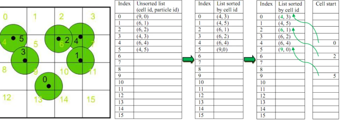
The implementation described in [12], is used in PhysX and Bullet and consists in parti-tioning the simulation space into a uniform grid (Figure 2.1), where the cell size is equal to the particle size (for different particle’s sizes, is the same as the largest size), so each object can occupy a maximum of 2d cells, whered is the number of dimensions (23cells in a 3D world). With this cell size, only four tests are needed for a 2D object and eight for a 3D object collision detection. The cell id on the grid is calculated for each particle based on its center points (for larger objects, it could be based on their bounding boxes positions). From this cell id, a hash value is computed to parameterize object cell position to CUDA’s grid. The cell hash value is stored along with the object id in an array which will be further transferred to the GPU. Once in the GPU, this array is sorted by cell hash value, using a parallel radix sort algorithm, described in detail by Scott Le Grand [11].
The next phase consists in signaling the cells containing particles in order to help the col-lision detection in the next step. This is achieved by writing in a new array (cell start array) the indexes in the sorted array where new cells appear. As shown in Figure 2.1, cells 4, 6 and 9 start on indexes 0, 2 and 5 respectively in the sorted array. To fill the array, threads (one per particle) gets the particle’s cell index in the ordered array and compares it with the cell index of the previous particle. If the indexes differ, it means that a new collision cell was found and the index is written.
Figure 2.1 Collision detection on the GPU: left image shows an example of bodies disposition on a 2D grid; right image shows how the array containing the particles and their cells on CUDA is before and after radix sort algorithm and how cell start array is filled
computes its hash value (for CUDA’s grid) and checks in the new filled array (cell start) if there are particles in that cell id. If the cell is not empty (contains an integer index representing its index in the ordered array), iterates over all bodies in the ordered array beginning on the index read from cell start array and tests for collisions.
Since this implementation is in CUDA architecture, developers are still restricted to NVIDIA’s GPUs. To achieve greater scalability, NVIDIA is considering the use of OpenCL in future PhysX releases.
However, OpenCL is already incorporated in Bullet’s SDK. Since version 2.77 (September 2010), one of Bullet’s features is the soft body and cloth library translated to OpenCL. So far, the current implementation only parallelizes the integration phase, forces computation and constraint solver and does not provide support fro collision detection or other advanced features. We can also check the Bullet’s OpenCL broad phase mechanism that uses a parallel Bitonic Sort algorithm for bodies’ hash sort, different from CUDA’s Radix Sort implementation. Bitonic Sort [16] is slower than Radix Sort [13, 26] for large data sets but performs better when has a small number of elements to sort. Moreover, for short arrays that can fit on GPU shared memory, execution is performed in a single kernel and take advantage of local memory fast access.
Presently AMD supports Bullet’s OpenCL developments, so it is expectable to see progress in this area, and in the meantime, we can follow the latest implementation updates on Bullet’s SVN [1].
2.2
Cloth Collision Detection
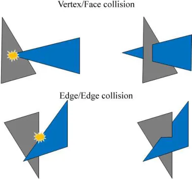
A cloth mesh is composed by a set of vertices, connected by edges, forming faces (usually triangles). Due to cloth complex structure and deformation capacity, collision detection is more difficult than for simple rigid bodies. To successfully identify collisions between cloth meshes and generic mesh objects (deformable or rigid), as well as cloth self intersections, two tests are needed (Figure 2.2), as demonstrated by Provot [25]:
• One vertex from one mesh intersects a face from another mesh (vertex/face collision).
• One edge from one mesh intersects an edge from another mesh (edge/edge collision).
Once more, testing all cloth triangles (vertices, edges and faces) against all obstacles’ trian-gles is not the best approach. It is a very time consuming solution and leads to unnecessary tests between distant triangles that have no chances to collide. To deal with this problem and accel-erate the collision detection phase performance we have to think in a more efficient strategy.
Figure 2.2 Collision types in cloth meshes: Vertex/Face collision and Edge/Edge collision
2.2.1 Spatial Enumeration
This technique consists in dividing the 3 dimensional simulation space, into smaller volume element boxes and assign each primitive (triangles for mesh based objects) to one of the boxes (based on triangle’s center point), allowing to check collisions only between primitives con-tained in the same or neighboring boxes. The grid is fixed during the simulation and we have to compute objects’ new cells within the grid at each time step. The volume organization generally varies between regular grids and hash tables (spatial hashing).
2.2.1.1 Regular Grids
also causes excessive triangles per box, decreasing the method’s performance.
The usual solution is to store each triangle in every cell it overlaps, creating a data structure larger than the initial set of triangles. A bounding volume is computed for each triangle (usually an AABB due to its simplicity) to easily identify the overlap cells. Then, in a second phase, we compute again each triangle’s overlapped cells through its AABB and check for intersection with other triangles in the same boxes. If two primitives overlap, a collision is detected and if they belong to the same object a self-collision is found.
Regular grids are simple and efficient, but they are not adaptive, which could result in many empty cells or many over-populated cells. This issue can be slightly improved with spatial hashing, since the hash table size is normally smaller then the whole grid.
2.2.1.2 Spatial Hashing
Spatial hashing [28] works by storing mesh vertices in a hash table (spatial hashing). Each vertex has a key, corresponding to its grid box identifier. Based on this key a hash value is calculated to obtain the hash table index where the vertex will be inserted. If two vertices with different key values obtain the same hash value, the insertion function will iterate over the hash table until it finds an empty position to keep one of the elements, which means that each array location will have vertices with identical keys (contained in the same cube). After filling the array with all vertices, starts the second phase of collision detection. All triangles are iterated and their AABB’s computed to discover the cells affected by the bounding volume. For each cell overlapped by the AABB, its hash value is determined and intersection tests are made between triangle and vertices in the same index (vertex/triangle test), as well as all the edges connected to the vertex (edge/edge test).
2.2.2 Bounding Volume Hierarchies
The basic idea is to partition the space occupied by the objects’ bounding volumes hierarchi-cally, storing it in a tree structure called Bounding Volume Hierarchy (BVH), used both for inter-object and self collision detection.
Each BVH refers to one mesh object, which means that to check if two deformable bodies are colliding we need to compare their BVHs. For a large number of bodies an exponential number of BVH evaluations will be needed, which is very time consuming and inefficient. One way to reduce that amount of tests is to enclose all objects with BVs and treat them like rigid bodies. Then it is possible to apply techniques like regular grids to check only the closest meshes.
2.2.2.1 Bounding Volume choice
volumes intersect with a few tests, depending on BV’s complexity. The most well known BVs for collision detection are Bounding Sphere, AABB, Oriented Bounding Boxes (OBB) andk -Discrete Oriented Polytope (DOP), each one with different characteristics. Figure 2.3 illustrates the equivalent 2D representations of these bounding volumes.
Figure 2.3 Bounding Volumes: Sphere, AABB, OBB and 8-Dop
Bounding Sphere [24] is the simplest BV and the easier to test for intersection. It is defined by a sphere centered on the object’s center with radius equal to the distance from the body’s center and its farthest vertex.
AABBs [29] and OBBs [10] are rectangular boxes that completely contain an object. An AABB is a box aligned with the coordinate axes and it only needs two tests per axis (six on total) to detect a collision with another AABB. OBB has an arbitrary alignment, frequently with object’s alignment for tighter fit. Collision detection is slower than for AABB but its update is relatively easier if the object just moves without altering its size (good for rigid bodies) because its OBB simply needs a rigid body transformation to follow body’s movement.
Another common type of bounding volume is thek-DOP. DOP stands for Discrete Oriented Polytope, which is the equivalent to a convex polygon in three dimensional space and the value ofkdetermines how many faces it has. An AABB (in 3D) is equivalent to a 6-DOP, having the planes’ normals oriented by the three dimensional axes. Values ofktypically vary between 6, 14 18 and 26, which is reflected on BV’s tightness. To detect an overlap between twok-DOPs only
ktests are necessary, at most, and the update cost per leaf node is proportional to the number of vertices inside the DOP, while it is in the order ofkfor internal nodes.
According to [17], k-DOPs offer the best solution due to their tight volume that limits the number of unnecessary elementary tests, paying off construction and update costs. In compar-ison, OBBs also provide a decent approximation to the set of primitives but have a prohibitive update cost. Nevertheless, in [17] it’s also referred thatk-DOPs should be composed by pairs of parallel planes, bounding the primitives along k/2 directions. This allows to compute k -DOPs using simple dot products between object’s vertices and the k planes’ normal vectors, minimizing the associated costs.
2.2.2.2 BVH Construction
Every mesh’s BVH is built in a pre-processing step, usually using a top-down approach. The BV envolving the entire mesh will match the tree’s root and its descendants result from successive splits in the ancestors’ BV. Usually, the arity of the tree depends on the number of axes split. For instance, one axis split results in a binary tree, two axes in a 4-ary tree (quadtree) and three axes in a 8-ary tree (octree). If we don’t want to divide along all the axes, the best option is often to cut where the BV is longer, in general on the BV’s center because it guarantees the smaller child volumes. Triangles intersected by the splitting plane are placed on the side where they have their centroid, or in alternative positioned on the BV with fewer primitives.
This recursive technique stops when it was reached a defined threshold on the quantity of triangles per volume. Besides its BV definition, a leaf node will also contain information about the triangles included in its volume.
2.2.2.3 BVH Traversal
In order to find possible collisions between two objects we must recursively traverse their BVHs and check for BV intersections, starting on both roots. Whenever a non-overlapping node pair is reached, the algorithm stops its recursive traversal in that branch. However, if an overlap is found and both nodes are leafs, their enclosed triangles are tested for intersection. If only one node is leaf, the following tests are between the leaf and the internal node’s children. Lastly, if the two nodes are internal, we choose one to step down and test its children. The best decision is to examine the node with smaller volume against the children of the node with larger volume (the decision can also be based on each node’s height in the tree or in the number of descen-dants), with the aim of quickly reach a stopping point in the algorithm (leafs intersection or no intersection at all).
Although this approach produces the right results, it’s possible to minimize the number of BV overlap tests, reducing this way the collision detection time. A technique introduced by Klosowsky in [17] exploits temporal coherence between successive frames to improve queries performance. The main idea is to keep track of the last (deepest) node pairs (one node from each tree) tested for overlap in the previous collision detection query, storing them in a front
At the beginning, the front will contain only the roots from the two hierarchies (last nodes traversed), but it will be updated during the simulation. It can be dropped, when a node pair in the front is replaced by one of its descendants: the last traversed until a non-overlapped node pair is reached or a pair of leaf nodes, meaning that a possible collision was found. The other option is to do araiseoperation, required when a particular node pair corresponding to an overlap between two BVs at the previous instant, no longer represents an intersection. In these cases, the node pair is removed from the front and it’s replaced by one of its ancestors (the first matching an intersection). To find the replacement pair, we choose one of the nodes from the removed pair to climb (usually the deepest in its hierarchy).
2.2.2.4 BVH Update
At each time step, a cloth object can move, deform or collide with another object, affecting its mesh arrangement and, consequently its BV and tree representation. This means that the hierarchy needs to be updated frequently to keep up with changes.
A “brute force” approach is to recompute the entire BVH at each discrete time step, which has obviously an exaggerated cost (O(nlogn)forntriangles) and will slow down significantly the simulation.
A better solution [20] is to refit the bounds of each BV in a bottom-up manner (O(n+logn)
forntriangles). Starting on leaf nodes, all triangles are checked to discover if their movement has placed their vertices out of the BV. In positive cases the BV is updated to fully enclose the triangles and changes are propagated up in the tree towards the root. Each BV is merged with its siblings and the result is used to refit their parent’s BV. We can reduce even more the update time by stopping refitting when the merged BV of all children is completely inside of their parent’s BV, before reaching the root.
However, successive updates result on a degradation of BVH performance in collision queries because primitives change their positions but the structure remains the same, leading to less tight fit BVs (with more empty space that could guide in false intersections). This aspect is specially noted when the cloth mesh suffers significant modifications during simulation time. To rectify the hierarchy and guarantee more efficient collision detections, we have to perform entire rebuilds from time to time. A simple approach is to rebuild the tree in pre-defined and fixed time intervals or number of steps, but it has a drawback: it is not adaptive to mesh defor-mations. The process used in [8] compares a node to its children based on their volumes and decides to rebuild the hierarchy when the ratio between them becomes very large.
by the fact that lower level nodes have more vertices shared by various triangles that are stored in more than one BV. Larsson refers that leveld=height/2 requires approximatelyn/2 vertex tests for n triangles, in other words, half the time needed to refit the BV when compared to leaf nodes. Then, the outdated nodes are repaired in the collision detection phase as they are needed. If the traversal reaches one of these nodes for an overlap test, the BV is recalculated in a top-down manner by splitting its parent BV. Obviously, this will result in some loss of time gained in the update phase.
Nevertheless, the same author improves this technique by introducing a dynamic update scheme that takes advantage of temporal coherence between successive frames in cloth simu-lation [19]. Instead of updating the upper half of the tree, the algorithm starts at the deepest nodes visited in the last collision detection query. The refitting is done the same way: the first BVs are recalculated based in their descendant set of primitives, the nodes above are built in a bottom-up style by merging child BVs and the outdated nodes are constructed during the col-lision detection phase. This scheme is similar to the front based mechanism used for colcol-lision detection improvement, providing a more accurate starting point for updating.
2.2.3 GPU Implementations
As it can be seen, collision detection involves many computations to correctly discover and treat primitive intersections, as well as time spent updating BV data structures, preparing them for the next collision query. This results in a major bottleneck in cloth simulation and GPU utilization emerges as an interesting option to accelerate its performance. Actual GPUs provide a large number of cores, capable of running a huge number of threads in parallel. These properties can be exploited by designing the right algorithms, choosing the best tasks to execute in parallel and the optimal way to distribute them.
Cloth collision detection has several phases that can be parallelized on GPU. One of them is BVH construction and is addressed in [7] where the authors describe two different construction algorithms.
The first one, called Linear Bounding Volume Hierarchy (LBVH), uses an efficient method based on Morton Codes to build hierarchies. The codes are calculated from primitives’ geomet-ric coordinates and used to map each primitive to its correspondent BV. First, a 2k×2k×2k
grid is established from the enclosing AABB of the entire geometry. Once this grid is made, a 3k-bit Morton Code is assigned to each cell by interleaving the binary coordinate values (Figure 2.4).
Figure 2.4 Example of 2D Morton Code grid.
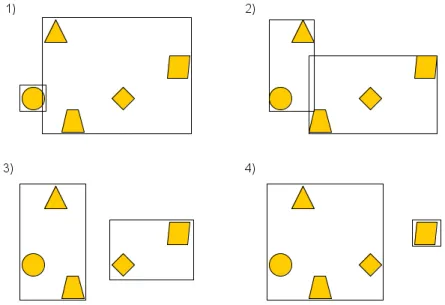
The second method uses the Surface Area Heuristic (SAH) to construct BVHs optimized for ray-tracing. The SAH consists in evaluating all possible split positions among all split planes and choose the one with lowest cost according to the ratio between its surface area and the number of primitives within it (Figure 2.5).
Figure 2.5 Possible object partitions along a single coordinate axis. SAH method tries to find the mini-mum total volume.
sorted, one thread updates the node’s bounding box information. In order to parallelize these steps, the authors propose a working queue approach to distribute the splits across all cores. Each block of threads reads a split object from the input queue, processes it (SAH evaluation, primitive sorting and BV update) and writes the resulting splits in the output queue. By using two work queues, one as input and another as output, in each construction level, we can avoid synchronization between them. In a binary tree the output queue should have two times the size of the input queue because we know that a split item can result at most in two new nodes. However, sometimes a split generates only one (one is leaf) or even zero new nodes (both leafs). These leaf nodes are written in the output queue as null objects because they don’t need to be divided in the next level, which forces a compaction before the next split kernel to ensure that only non leaf nodes remain in the queue. The compacted queue is then sent as the new input queue for the next split kernel invocation and the procedure is repeated until all nodes are divided.
Due to its simplicity and high parallel scalability, the Morton code based algorithm can build hierarchies extremely quickly. It just performs a sorting operation to bucket the primitives to their correspondent nodes, avoiding the evaluation and selection of a split point. Although being the fastest construction method, it does not achieve the best BVHs for collision detection. The reason is that the splitting point is always static and does not adapt to the distribution of the geometry, which could lead to very non-balanced trees causing an increase of work during the collision detection phase.
The SAH construction algorithm performs a more balanced partition of the primitives across the hierarchy. This scenario can be favorable during the BVH traversal by reducing the number of levels covered to detect a collision, as well as the number of elementary tests done in the next phase. As a disadvantage, it has the lack of parallelism between processors in the first splits and the lower resources utilization in very small splits at the last hierarchy levels, plus higher compaction costs. To solve the first issue, the authors present a hybrid algorithm that uses the LBVH method in the initial levels to maintain the parallelism and processes the remaining active splits with the SAH scheme, without compromising the hierarchy quality. In order to deal efficiently with the small splits, the kernel writes those splits to a local work queue (since local memory access is fastest than global memory) and processes them at the last step in one single run, using as few threads as possible (32 in this case) to reduce memory accesses and memory bandwidth.
However, despite these advantages, this solution does not take maximum benefit from the large number of threads available. The main problem is that collisions in a cloth mesh can occur in localized regions, producing high variance in the number of overlap and collision tests that each thread has to do. In other words, some threads can process branches with few or no intersections at all and terminate their work and yet, need to wait for other busy threads to finish, resulting in many idle threads and less productive work. Furthermore, higher level nodes are visited and tested repeatedly by various threads, which is clearly unnecessary. To prevent these problems, some techniques were introduced, mostly based on work queues, for a better task distribution.
The implementation presented in [21] uses one work queue per core (shared by several threads) to store pairs of BVs to test for overlap. Each work queue is initialized with one pair from the front (if the number of threads are larger than front size, there are threads without initial nodes), making each core traversing a different branch and avoiding repeated tests in the same nodes. At each iteration, a thread dequeues one node from its shared queue (queues are processed in parallel using atomic operations) and checks it for intersection. If the two BVs overlap, two new nodes are generated (or four nodes, depending if we choose to descend from one or both nodes of the pair) and enqueued again. Whenever a work queue becomes full or empty, making impossible further work, a global counter, visible by all threads, holding the number of idle cores, is atomically incremented and the kernel execution is stopped in that core. Every thread reads that counter after processing a node pair and checks if its value already exceeded a user-defined threshold (50% of idle cores is a good value). If yes, the work queue is written to global memory and the kernel is aborted. After all cores aborted or finished their executions, a kernel is launched to examine all work queues and assign the same number of tasks to each one. The algorithm is repeated until every possible colliding pair is processed.
However, the algorithm performance depends on front size. A small front does not allow for great parallelism by leaving too many threads without work, resulting in a modest speed-up when compared to a sequential approach.
A similar implementation is presented in [15] using both multi-core CPU and GPU archi-tectures to deal with CCD.
On a second phase, a single CPU thread sends segments containing thousands of triangle pairs to the GPU. The collision tests between triangles are then performed in parallel by the device and results are sent back to the CPU.
2.3
OpenCL framework
OpenCL [23, 9, 5] is a framework for parallel programming that allows developers to write efficient code in a C based language capable of running on devices like GPUs. It is similar to CUDA, but unlike this, OpenCL is not restricted to NVIDIA’s GPUs, providing a standard solution. Moreover, OpenCL is device agnostic, which means that its utilization is not confined to GPUs but to every device that meets OpenCL requirements.
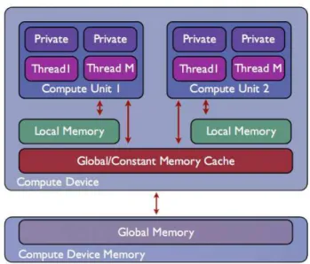
An OpenCL application runs on a host (usually the CPU) that is connected to one or more devices. A device is divided into one or more compute units (in a GPU it corresponds to a set of multiprocessors called Streaming Multiprocessor (SM)) and each compute unit can have several processing elements (equivalent to the multiple cores within a multiprocessor, each one called Streaming Processor (SP)).
The host executes a program that manages the functions (kernels) that run on devices. It allocates memory space on the device and transmits the data required to kernel execution. Each instance of a kernel is called a work-item (equivalent to a thread) and each work-item runs the same kernel code. Work-items are grouped into work-groups, providing a more coarse-grained organization. Each work-group is executed by one compute unit and all its work-items execute concurrently.
Work-groups initially are distributed to the available compute units (multiprocessors) and as they finish, new work-groups are assigned to the idle multiprocessors. The threads within a multiprocessor are executed in groups of 32, namedwar ps. Those 32 threads run one common instruction at a time. Work-groups are organized in anN-dimensional grid (whereNis one, two or three) that limits the total index space available (Figure 2.6) and have IDs to identify their position inside the dimensional space. Likewise, items have local IDs within their work-group and global IDs along the whole space. These identifiers can be very useful, for example to assign to each thread a different position on an array, enabling parallel access. Work-items can access data from different memory locations in the device, as we can see on Figure 2.7.
• Global memory: each thread can read or write from global memory, but only the host can allocate space. It is shared by all work-items from all work-groups.
• Constant memory: it is initialized on the host and remains constant during kernel execu-tion, which means that is a read only memory.
• Private memory: it’s a private memory location to each work-item, but significantly smaller.
Figure 2.6 Index space orgainzation on OpenCL: example of work-item and work-groups within a two dimensional index space
Figure 2.7 Memory architecture in OpenCL device: private, local, constant and global memory loca-tions
it’s possible to explicitly enforce memory consistency in some point during the execution, by invoking a thread synchronization. Calling a barrier instruction guarantees consistency in local and global memory within the same work-group.
In conclusion, OpenCL provides a flexible way to take advantage of GPU resources and distribute the computational work efficiently across several cores. This parallelization should be very useful in the cloth collision detection context, since the meshed objects are usually composed by large amounts of primitives, which can result in a high number of collision tests. By using the GPU, it is possible to distribute each primitive or set of primitives within an object across several threads during a BVH construction, BVH update or narrow phase collision detection, while in the BVH traversal we can perform BV overlap tests in parallel. Besides the high parallelism, it is also possible to execute operations in local memory, reducing the memory access timings.
3.1
Introduction
In this chapter we present an implementation, based on OpenCL kernels, to handle collision de-tection on the GPU. This implementation deals with discrete collision dede-tection between a piece of cloth and other mesh objects. However, we did not focus on self collisions in the deformable model neither on the collision response mechanism. This GPU kernels were integrated in the cloth simulator developed in [6], which allowed us to have a basis for comparison between CPU and GPU performances.
The kernels developed include the construction of a BVH for each simulation object, two different approaches to traverse the hierarchies and find the colliding primitives, a method to perform parallel elementary tests between primitives and a BVH update scheme.
In the following sections we will explain in detail all of these kernels and our implementation choices.
3.2
Bounding Volume Hierarchy Construction
3.2.1 BVH Construction Kernel
As we have seen in the previous chapter, an option to efficiently detect collisions between meshed objects is to map them into a BVH. We have chosen to use binary trees in our BVH implementation because they are simpler and faster to build. Specifically, for each tree level we only need to perform one split per node, generating two different subsets of primitives.
Concerning the hierarchy construction, the process is composed by three main phases, for each node: choosing the split point within the BV; reordering the primitives either for the left or right sides of the split point; computing the two new child BVs (in a binary tree) from the reordered primitives.
However, to build the root node we only apply the last step, since the root is built from the entire set of primitives while the remaining nodes are defined from their ancestors’ primitives. To simplify, we have different kernels for the root and for the rest of the hierarchy nodes. In both construction kernels, each BVH node is built by one work group to ensure that no synchronization between different groups is required.
3.2.1.1 Root Construction Kernel
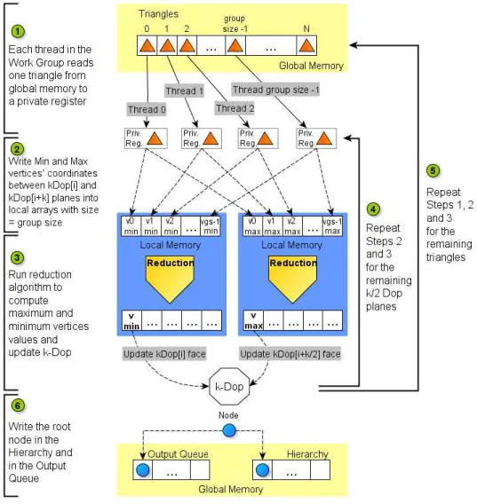
To construct the root node, each thread from the assigned group reads a primitive from global memory to a private register, in order to create a bounding volume from their vertices’ coordi-nates, as shown in Step 1 of Figure 3.1 and detailed in Appendix A.3.1.
coordinate values of the vertices from the primitives along several directions. For example, to calculate the two BV planes parallel to x axis, we need to find the smaller and the higher vertices’ values along that axis. To compute the threshold values in the kernel, each thread writes into a local array (with size equal to group size) the minimum value of its primitive’s vertices along the chosen direction (Step 2). For instance, if the primitive is a triangle and the direction is thexaxis, we check the tree vertices’ coordinates and choose the smallest value of
x. After the array is completely filled, the entire group performs a reduction operation [13] to obtain the minimum value and updates one BV face with it, as indicated in Step 3 of Figure 3.1.
Figure 3.1 Steps to build the root node from a set of triangles
We use a 18-Dop as BV and the faces are stored in 18 length array where the minimum and maximum values in a given direction are stored in positionsiandi+k/2 respectively, with
stored in positions 0 and 9). The process is then repeated for the maximum value in the same direction and spread to all the remaining directions needed to compute the BV faces (Step 4). In our case, to define all the faces of a 18-Dop volume, the reduction is executed over x, y, z,
x+y, x+z, y+z, x−y, x−z andy−z directions. If the number of primitives is larger than group size, we repeat the above steps for the remaining primitives, processing them in blocks with the group size (Step 5).
When all the BV values are computed, one thread is responsible to add some information fields to the node, such as parent, left child and right child indices, node’s level in the hierarchy or start and end indices of the primitives within the volume. The new node is then written to the hierarchy array and also to a work queue to be processed during the next kernel invocation (Step 6 in Figure 3.1).
In the root construction kernel we also have to initialize an array with the primitives’ indices. At the beginning, the indices in the array correspond to the primitives’ order in their array. However, during the construction process we have to reorder primitives’ indices to set them in the correct BVs. Instead of change the primitives array order, we switch their indices in the primitives indices array. The reason why we do this, has to do with the fact that the primitives array on the GPU is not synchronized with the CPU version. Once the triangles are created on the CPU, they maintain their positions in the array during the entire simulation and we don’t change their indices to match modifications done in the kernels. Every time the primitives are updated (acceleration, velocity, position, etc) on the CPU, we transfer them to the GPU and access them through the primitives indices array. This way it is possible to utilize the input data and read the correct primitives according to the BVH organization. Unfortunately, this represents an extra step each time we need to access a primitive because we first have to load its index and then the corresponding primitive. However, the initialization process is easily done in parallel by all the threads in which each thread writes its identifier (global id) in the same index (value 0 in index 0, value 1 in index 1, etc).
3.2.1.2 Remaining Hierarchy Construction Kernel
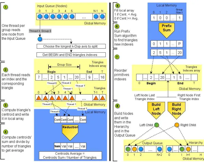
After having the root node built and the indices array initialized, the remaining nodes can be constructed from their ancestors. The task is accomplished on a level by level basis. The following construction kernel invocations have as input a queue created in the previous level with all the non leaf nodes (Figure 3.2 and Appendix A.3.2).
Each input node is read by a different work group which will subsequently split it in two child nodes. Therefore, one thread within the group loads the node from global to local memory and then the remaining threads read it to their private registers (Step 1 in Figure 3.2). Once all threads have their copy of the node, the process of splitting and creating new nodes can start. To choose the best plane to divide the node we use a method presented in [17] that proved to be the fastest among other possibilities: pick the plane where there is the longest distance between two oppositek-Dop faces. This is achieved by computing the difference betweenk-Dop[i] and
Then we need to select a good position for the splitting plane. One possibility is to split by the median, in other words, sort the primitives based on their centroids and assign the left half to the left node and the right half to the right node. The Bitonic Sort [16] algorithm is an option to order the primitives that performs well on small sized arrays (capable of being sorted inside a single group) but it is sub efficient for large sequences when compared with the Radix Sort [13, 26]. Although radix sort is particularly suited for integer keys (specially with a small number of bits), it is also possible to sort floating point values by converting them into sortable unsigned integers [14, 27] through a very inexpensive operation. By using this algorithm, dividing the primitives by the median may be an efficient splitting method. However, results in [17] showed that splitting by the mean always produces a hierarchy with smaller total volume than using the median, despite generating less balanced hierarchies.
Based on that, the decision was to use the mean method and compute the average of primi-tives’ centroids in the chosen plane through a reduction algorithm and sort them into either the left or right sides using a scan algorithm. To perform that task in parallel each thread reads one triangle index (in the range between the node’s primitives’ indices) and loads its subsequent triangle (Step 2). Then extracts its centroid in the chosen plane (given by the average between all primitive vertices’ coordinates in that plane) and writes it down in a local memory array, as illustrated in Step 3. The work group runs a reduction to find the centroids’ sum and divides it by the number of primitives to get the average point (Step 4).
After that, it is necessary to reorder primitives’ indices based on the split point. If the triangle’s centroid value is lower than the split point, a 1 is written into a local array, otherwise it’s filled with a 0 (Step 5). This array is used to perform a prefix sum and from the values obtained it’s possible to calculate the new positions for primitives’ indices (Step 6). Left sided indices are placed in consecutive positions from left to right, starting from input node begin index, and the same applies to right sided indices, in the opposite way, starting from end index, as showed in Step 7 of Figure 3.2. If the number of node’s primitives is larger than the group size, we need to keep processing indices in blocks with group size, starting again from Step 2.
At the end, we must have all the left and right new nodes’ indices ordered between the input node bounds and in addiction know the index where one ends and another begins. The next stage (Step 8) consists then in constructing both left and right BVs with their newly primitives through the same mechanism used in root building (Figure 3.1), with the difference that the left child is built with primitives in the range ofbeginandlast le f t node indexand the right child with the primitives in the rangelast le f t node index+1 toend.
Hereafter, one thread sets in both nodes their parent index as the input node index, as well as their left and right child indices. If the node has less primitives than the threshold defined for a leaf, its children indices are set with -1 value, signaling that it is a leaf node. In addiction, itsbeginandendfields, pointing to the primitives indices array, are also saved to be used in the next split. They are finally written in the hierarchy and in the output queue to be processed in the next kernel invocation (Step 8).
3.2.2 BVH Construction Kernel Optimizations
The above construction kernel has two main bottlenecks, as evidenced in [7]. One of them is the large number of nodes with few primitives in the lower levels of the hierarchy. The second bottleneck happens in the initial hierarchy nodes, due to their large size and the lack of parallelism by assigning only one work group per node.
Figure 3.3 Construction timings per level for for the Happy Buddha model: construction is slow in the first levels due to the nodes’ size, while in the last levels the performance decreases due to the queue size.
In the following subsections we introduce three measures to reduce these performance is-sues.
3.2.2.1 Adaptive Work Group Size Optimization
In our construction kernel, each node is split by an entire work group. As we build new hierarchy levels, the amount of primitives per node decreases. When the number of primitives in the node is less than the group size we can have many idle threads (or threads doing unnecessary work) revealing a poor utilization of work group parallelism, that is reflected in a decrease of performance.
To solve that problem we need to adapt the work group size to the number of primitives per node, in order to have the maximum use of all threads. Our solution was to estimate the average node size at each level and reduce the group size to follow that value. The number of threads within each work group should be always higher than the node size and also a power of two, since it is a necessary condition to execute the scan and reduction algorithms. We compute the average node size at each level by dividing the total number of primitives by 2level−1. Whenever
that value is above the work group size, we round it up to the next power of two and set it as the new work group size.
3.2.2.2 Small Splits Optimization
To split very small nodes we use an algorithm based on the idea presented in [7] to deal with small splits. The idea is that each small node is processed by a single thread using its private memory registers, avoiding the local memory accesses and the synchronization needed to split larger nodes across all group threads (kernel detailed in Appendix A.3.3).
In the construction kernel we define a threshold value for the maximum number of primitives contained in a small node. During the kernel execution all the nodes above that threshold are filtered into a local array instead of being split by the current work group. Once all nodes from the input queue are processed, each thread within the group loads and splits individually one or more small nodes from the local array. By individually we mean that all the steps needed to split the node and generate its two child nodes are made sequentially by only one thread. With this method there are several threads doing work in parallel and less idle threads. Nevertheless, the threshold value should be smaller than the group size in order to compensate the increase of work per thread when compared to a split executed by the entire work group. In the end of the kernel, one thread per group atomically increments a global counter with the number of small splits done in that group, to account the total of small nodes in that level.
Before the next kernel invocation, we compare the number of small nodes with the queue size: if the small nodes exceed a percentage limit (another defined threshold) in the queue, we invoke a different kernel where each thread begins immediately by reading the nodes from the input queue in parallel, avoiding the filtering process (conducted by only one thread per group in the construction kernel). In other words, each node will be processed by a single thread instead of being processed by an entire work group, which results in more work per thread, less idle threads and no need for synchronization of work group threads during the kernel execution. This modification in the construction mechanism represents a considerable improvement in terms of performance, as we will see in chapter 4.
3.2.2.3 Large Nodes Optimization
In this section we address the bottleneck problem in the top hierarchy levels by introducing an improved construction mechanism for large nodes. Instead of assigning a single work group per node, we want to use several work groups, cooperating to build those large nodes.
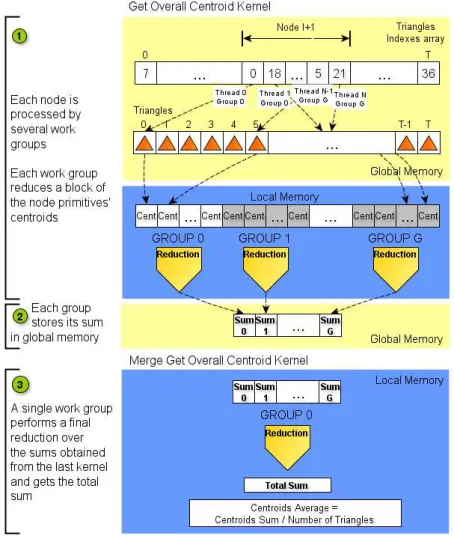
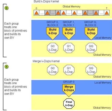
The basic idea is that each group should process a block of node’s primitives (or more, de-pending on the number of work groups assigned) during the building process. The construction process can be divided into three main phases: choose the split point, reorder the primitives and build the two new child nodes. Each one of this phases is done through parallel algorithms such as scan and reduction. Note that for the root node we only have to perform the last phase, since we already have the initial set of primitives ready for thek-Dop construction.
sums array to find the total sum and divide it by the number of primitives to get the mean point, as illustrated in Figure 3.4 - Step 3 (the loading of the block sums array from global to local memory was ignored in the figure). In alternative, we can use only one kernel: in the first kernel, one thread per group increments a global counter with the total sum through atomic operations.
Figure 3.4 Kernels to get the split point for large nodes. The first kernel is executed by several groups. In the second kernel, a single group performs a final reduction to obtain the overall centroid.
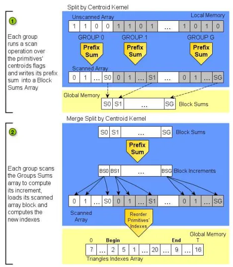
were omitted in the figure), loads its scanned array block and computes the new indices with that information, either for the left and right side indices, as illustrated in Step 2 of Figure 3.5.
To build the BV each group treats one block of primitives and builds its own BV (Step 1 of Figure 3.6). In a second kernel, one group performs a merge of all the BVs and define the final volume (Step 2 of Figure 3.6).
Figure 3.5 Kernels to reorder primitives’ indices. In the first kernel each group scans the centroids’ flags array and saves its block sum. In the second kernel, each group obtains its block increment by scanning the block sums array and computes the new indices.
Figure 3.6 Kernels to build a BV from several blocks of primitives. In the first kernel each group builds a BV from its block of primitives. In the second kernel, one work group merges all the BVs constructed in the previous kernel and defines the final BV.
3.2.3 Compaction Kernel
3.2.3.1 Compaction Kernel for Small Arrays
Whenever the construction kernel creates leaf nodes, it is necessary to perform a compaction in the output queue, leaving only the internal nodes to be split in the next construction kernel invocation. For a small queue, capable of being processed by only a single work group at once, we only invoke one work group (Figure 3.7 and Appendix A.3.5.1). In our kernel, each thread processes two nodes, so the queue can have up to twice the size of the work group.
Figure 3.7 Compaction kernel for small arrays, executed by a single work group
we run a parallel scan algorithm (prefix sum) to compute nodes’ new indices. With the array scanned, threads write the internal nodes in their new indices, inside the new output queue.
However, besides removing leafs from the work queue, compaction has an additional func-tion of redirecting some nodes’ child indices. This comes from the fact that leaf nodes do not have children, which would create empty spaces between the nodes of the next level of the hierarchy.
3.2.3.2 Compaction Kernel for Large Arrays
To scan large arrays we use a different method executed across several work groups simulta-neously and divided into three distinct kernels (for more details, please see Appendix A.3.5.2). In the first kernel, the queue is divided into smaller blocks, capable of being processed inside a single group at once. Each group scans its block and writes the total sum (corresponding to the number of non leaf nodes) into an array of block sums in global memory, as illustrated in Steps 1 and 2 of Figure 3.8.
Figure 3.8 Compaction for large arrays: in the first kernel each group scan a block of nodes from the queue, creating a block sums array
Figure 3.9 Compaction for large arrays: in the second kernel a single work group scans the block sums array, generating an array of block increments
that case, each work group would have to fill an extra block sums array for the block increments array, that would have to be also scanned in the last kernel. Another option could be computing the block sum scan in the last kernel, without this intermediate kernel. However, this would require that every work group had to perform the same scan operation over the entire array. That situation would be particularly bad if we have more work groups than multiprocessors, meaning that each multiprocessor has to run the same scan operation for multiple groups.
Figure 3.10 Compaction for large arrays: in the third kernel the group threads add the block increment stored in their work group index to their previously block scanned values and save their nodes in the new indices
Finally, we run a third kernel in which all the group threads add the block increment stored in their work group index to their previously block scanned values (Step 1 in Figure 3.10). With those values, each thread with a non leaf node enqueues it in the right position and corrects its child indices (Step 2).
3.3
Broadphase Collision Detection Kernel
3.3.1 Simple Broad Phase Collision Detection
The kernel responsible for this operation receives as input the object’s hierarchies and re-turns as output a list with all the potential pairs of colliding primitives. The first step is done sequentially by one thread that reads both root nodes and tests their BVs for overlap (Figure 3.11 and Appendix A.4.1).
Figure 3.11 Example of hierarchies traversal starting from the roots. When two internal nodes overlap, we write four new node indices into a local queue for further processing.
memory space is insufficient to keep a large amount of geometry data. After inserting new nodes on local queue a local counter (write index) is also updated, signaling the index of the last enqueued element, in order to avoid reading positions out bounds.
From now on the algorithm can run in parallel by several threads. A thread with an identifier smaller than the difference between read and write pointers can dequeue a pair of indices and load their corresponding nodes from the hierarchies, while increases the read index value. If an overlap exists, the write pointer is incremented by the number of elements added and the indices are placed in the queue. If one node from the overlapping pair is a leaf, we enqueue the indices from the leaf together with the indices from the other node’s children, resulting in just two new items (Figure 3.12).
Figure 3.12 Example of hierarchies traversal starting from the roots. When one of the overlapping pair is leaf, it results in two new node indices in the local work queue.
To synchronize this process and prevent different writes on the same position, each thread uses atomic operations to change pointer’s values.
In case both nodes are leafs, the thread loads nodes’ triangles and stores all the possible pairs of colliding primitives into a global array (Figure 3.13). To ensure that each pair is written in an empty position, it is necessary to atomically increase the array pointer into the last index saved.
The algorithm ends when the read index reaches the same value of the write index, meaning that the processing queue is empty.
Figure 3.13 Example of hierarchies traversal starting from the roots. If two leafs overlap, we write their pairing primitives into a result array in global memory.
kernel would perform, at most, four times better than the single group method.
To increase the number of initial nodes to test and launch several work groups in parallel we could use a different method, by starting the traversal in lower levels. For instance, we could begin in the first levels with leaf nodes and descend the tree from there. The number of initial overlap tests would be given by the total amount of node pairs from both starting levels of the hierarchies. In an extreme case, this represents testing all the leaf pairs in both hierarchies. It could be a good approach if the majority of the objects’ primitives are colliding, when com-pared to always start from the root nodes but even so, it might result in many unnecessary tests between far away BVs and the algorithm will perform worst when the objects do not collide.
Another strategy could be using the CPU to perform the tests in the first levels of the hi-erarchy (with fewer nodes), generating a set of colliding pairs of nodes in a sufficient number to distribute among several work groups. By doing this, we were only sending to the GPU, as input, pairs of nodes that really intersect, avoiding unnecessary tests between faraway BVs like in the above method.