Ana Isabel de Figueiredo Alves dos Reis Poças

Departamento de Ciências e Engenharia do Ambiente

Fouling of a drinking water system in relation to hydraulic

circumstances and customer complaints

Ana Isabel de Figueiredo Alves dos Reis Poças

Dissertação apresentada na Faculdade de Ciências e Tecnologia da Universidade Nova de Lisboa para obtenção do grau de Mestre em Engenharia do Ambiente, Perfil Sanitária

Orientador científico: Prof. Doutora Leonor Amaral

Acknowledgements

The thesis has been carried out with the collaboration of the Research Department of Oasen Drinkwater in Gouda and the Water Management Department of the Technische Universiteit of Delft, The Netherlands, between July 2007 and December 2007.

I am very grateful to my supervisor Dr. Ir. Jan Vreeburg for making this possible and for all the support, advice and contribution for the development of my work.

I would also like to express my gratitude to Ir. Maarten Lut, with whom I have discussed all the measurements, research topics and for his help in everything I needed.

Special thanks to Dr. Ir. Leonor Amaral, who made all of this possible, and for her devotion towards the good outcome of my work.

I would also like to thank to all of my friends in Portugal and in The Netherlands, and my colleagues at Oasen.

Fouling of drinking water system in relation to hydraulic circumstances and customer complaints 4 Abstract

In a “perfect” drinking water system, the water quality for the consumers should be the same as the quality of the water leaving the treatment plant. However, some variability along the system can lead to a decrease in water quality (such as discolouration) which is usually

reflected in the number of the customer complaints. This change may be related to the amount of sediment in the distribution network, leading to an increase in turbidity at the water supply. Since there is no such thing as a perfect drinking water system, the behaviour of particles in a drinking water network needs a suitable approach in order to understand how it works.

Moreover, the combination of measurements, such as turbidity patterns and the Resuspension Potential Method (RPM) aid in the prevention of discoloured water complaints and

intervention in the treatment upgrade or the network cleaning.

Besides sediments there is also bacterial regrowth in the network, which is related to the water quality and distribution network characteristics. In a theoretical drinking water system higher velocities, temperature and shorter residences times lead to wider bacterial growth. In this study we observe velocity and residence steady-states and bacterial does not seem to be related to either.

It can be concluded that adequate measurements of RPM, customer complaints and bacterial

Resumo

Numa rede de abastecimento “perfeita”, a qualidade da água que chega às torneiras dos consumidores deveria ser igual à que sai da estação de tratamento. No entanto, existem algumas variáveis de “percurso” que fazem com que nem sempre a qualidade que chega às torneiras seja a desejável, o que se traduz, normalmente, em reclamações dos consumidores. Esta alteração na qualidade pode estar relacionada com a quantidade de sedimento existente nas tubagens o que, geralmente evidencia a presença de turvação nessa mesma água. Como os sistemas não são perfeitos, e com a vista a uma correcta modelação, demonstra-se a

necessidade de um conhecimento mais aprofundado sobre o comportamento das partículas numa rede de abastecimento. Assim, a combinação de resultados utilizando padrões de turvação e medições do Resuspension Potential Method (RPM), ajuda a prevenir reclamações dos consumidores e a intervir no controlo da qualidade da água e limpeza da rede.

Num sistema de abastecimento de água teórico, o desenvolvimento bacteriano aumenta com a velocidade, temperatura e tempos de retenção mais curtos. Neste estudo verifica-se a

existência de patamares de velocidade e de tempos de retenção, sendo o crescimento bacteriano independente dos mesmos.

Conclui-se, assim, que a aplicação prática de técnicas de medição apropriadas leva a um

Fouling of drinking water system in relation to hydraulic circumstances and customer complaints 6 TABLE OF CONTENTS

Fouling of drinking water system in relation to hydraulic circumstances and customer complaints 8 List of Figures and Tables

Fig. 1-1 Examples of discoloured waters

Fig. 1-2 Type and percentage of customer complaints in 2006 at Oasen Fig. 1-3 Particle-related processes in the drinking water distribution system

Fig. 1-4 Development of the discolouration risk in the DWDS based on the particle-related processes Fig. 2-1 Transportation and generation of suspended solids

Fig. 2-2 Biological development under different cleaning frequencies and treatment standards Fig. 3-1 Oasen´s municipalities

Fig. 3-2 Treatment plants´ supply areas

Fig. 3-3 Cumulative frequency based on measured hour online turbidity at De Laak´s transportation area

Fig. 3-4 Average hour turbidity at De Laak

Fig. 3-5 Principle of the Resuspension Potential Method

Fig. 3-6 Typical RPM turbidity trace resulting from an RPM test Fig. 3-7 Example of the RPM measurements done in Jacobswoude Fig. 3-8 Typical RPM turbidity traces

Fig. 3-9 Average turbidity for the 4th -9th minute average: correct, overestimated and understimated Fig. 3-10 Process for the registration of a technical complaint at Oasen

Fig. 3-11 Hotspots for the Aeromonas in 2006

Table 3-1 Example of ranking the RPM for discolouration using the Dr Lange Ultratub equipment at the flushing point

Table 3-2 Boundaries for the rank of the discolouration risk from the RPM

Table 3-3 Threshold for discoloured water complaints and technical complaints in total Fig. 4-1 Online monitoring of turbidity at De Laak

Fig. 4-2 RPM, cleaning frequency and number of discoloured water complaints at Rodenhuis Fig. 4-3 RPM, cleaning frequency and number of discoloured water complaints at De Laak Fig. 4-4 Number of discoloured water complaints

Fig. 4-5 Performed cleaning activities and treatment improvements in relation to the number of discoloured water complaints per 10 000 inhabitants

Fig. 4-6 Effects of improving treatment and cleaning the network at De Laak Fig. 4-7 Percentage of hotspots and temperature

Fig. 4-8 Aeromonas and residence time

Fig. 4-9 Aeromonas and residence time between 13 and 17 ºC Fig. 4-10 Aeromonas and flow velocity

Fig. 4-11 Aeromonas and flow velocity between 18 and 20 ºC Table 4-1 Cumulative frequency at Rodenhuis and De Laak Table 4-2 RPM measurements at Rodenhuis

Table 4-3 RPM measurements at De Laak

Table 4-4 Number of complaints per 10 000 inhabitants

Table 4-5 Number of complaints per 10 000 inhabitants at each treatment plant Table 4-6 Percentage of hotspots

Table 4-7 Percentage of hotspots and temperature Fig. 5-1 Monitoring cast-iron and PVC networks Fig. 5-2 RPM measurements at Leiderdorp

Fig. 5-3 Maximum and minimum RPM scores from the cast-iron pipes Fig. 5-4 Maximum and minimum RPM scores from the PVC pipes Fig. 5-5 Adjusting RPM

1. Introduction

1.1 Particles in the drinking water system

A substantial part of water quality problems is associated with the accumulation of particles in drinking water networks. This accumulation of particles may be caused by the water coming from the treatment plant or from the corrosion of unprotected cast-iron or steel mains [J. Vreeburg, et al., 2007].

Particles incoming from the treatment plant represent a significant source of the suspended solids that may settle, creating a layer of sediment or resuspending, depending on the flow dynamics [Vreeburg, 2007]. Flow velocity changes have great influence on the shear stress and affect settling and resuspension [J. C. van Dijk,et al. 2004].

Settling and resuspension phenomena are described by Stokes and Shields formulas. Berlamont has developed a Shields-theory on the resuspension of particles, having experimentally reached the formula that describes the critical velocity for resettling and

resuspension in sewer pipes:

(

)

(

)

w

u



g





d







Equation 1. 1.

Where:

Critical shear stress velocity (m/s)

Berlamont coefficient (0, 8 for resuspension)

Density of the particle (kg/m3)

Density of the water (kg/m3)

Diameter of the particle

The relation between critical shear stress velocity u* and average velocity v in the pipe is

Fouling of drinking water system in relation to hydraulic circumstances and customer complaints 10 *

/ 8

u

v





Where:

Critical shear stress velocity (m/s)

Average velocity (m/s)

Darcy-Weisbach friction factor

With a course estimation of λ=0,02, representative for a pipe with a diameter of 100 mm and a Nikuradse roughness of 0,1 mm, the result of the previous equation is a relation of v=20.u*cr.

Under normal circumstances velocities at the distribution networks are low, which explains the sediment settling according to Berlamont. Resuspension processes from previous studies showed that particles may resuspend when velocities are higher than 0, 35 m/s [Vreeburg, 2007].

1.2 Nature of the discoloured water and customer complaints

The settling and resuspension of particles are related to the fouling of the drinking water system, being the resuspension of accumulated particles the main cause for an increase in the number of customer complaints. Discoloured water is the naked eye of brown/black/red

colour in the water from the tap which, in a strict water quality sense, is evidence of dissolved contaminants. The particulate matter experienced by the customer as “discolouration” is turbidity [Vreeburg, 2007]. Turbidity is measured in Nephelometric Turbidity Units (NTU) or Formazine Turbidity Units (FTU)1.

Discoloured waters can be brownish, black or red, which suggests different origins of discolouration (see Fig. 1-1).

1

Fig. 1-1 Examples of discoloured waters [Vreeburg, 2007]

Figure 1-1 clearly shows the importance of the discoloured water complaints in the total

number of complaints related to a drinking water system.

Fig. 1-2 Type and percentage of customer complaints in 2006 at Oasen Drinking Water Company, Gouda, The Netherlands

Fouling of drinking water system in relation to hydraulic circumstances and customer complaints 12 1.3 Particle-related processes in the drinking water distribution system

Discolouration is associated with the mobilization of accumulated particles in the distribution network. Particles can either enter the distribution network as background concentrations of organic and inorganic material [Lin and Coller, 1997; South-East-Water, 1998; Kirmeyer et al. 2000; Slaats et al. 2002; Ellison, 2003] due to incomplete removal of suspended solids at the treatment plant [Gauthier et al. 2001; Vreeburg et al. 2004b] or from processes occurring at the distribution system. All the particle-related processes happening in the network are presented in Fig. 1-3.

Fig. 1-3 Particle-related processes in the drinking water distribution system [Vreeburg, 2007]

The underlying cause of discolouration can be explained by this framework, assuming that discoloured water is formed by: particles attached to the pipe wall, particles imported (from treatment or outside the network) or produced at the network. Particles come from the treatment plant and may settle or resuspend. If hydraulic circumstances change, shear stress may increase and cause the mobilisation of particles leading to customer complaints. The

network hydraulics and the composition of both suspended particles and deposits layer, determine how high the discolouration risk is. For a complaint to occur it is necessary to have a large quantity of sediment together with a hydraulic event, plus the customer’s motivation to complain. Under these circumstances, the threshold for complaining is around 10 FTU [Vreeburg, 2007].

that the treatment plant is the major cause for discolouration, rather than corrosion [Smith et al, 1997; McNeil and Edwards, 2001].

One of the actions to prevent complaints is to limit the amount of resuspendable sediment in the network by cleaning it. However, it can be a bad operational image if proper requirements are not considered, leaving the discolouration risk at the same level or at a slightly lower one [Antoun et al., 1997]. A good cleaning method should decrease the number of discoloured water complaints and have a reasonable cleaning frequency.

The hypothetic development of the discolouration risk in the network is sketched in Fig 1-4.

Fig. 1-4 Development of the discolouration risk in the DWDS based on the particle related processes [Vreeburg, 2007]

On the vertical axis discoloration is quantified to a tangible value, that can be reached by the amount of loose deposits in the network. The horizontal axis represents the time needed for the water to increase the discolouration risk up to critical levels. From the picture, the discolouration risk is determined by the amount and mobility of loose deposit in the network, originated by the particle related-processes (Fig. 1-3).

Within the possible methods2, water flushing has been the applied method for the networks´ cleanup. The problems associated to conventional flushing are: the increased number of complaints during and immediately after flushing and a minimal short-living water quality benefit, but also a potential for increased coliform occurrences. In several locations conventional flushing was refined to unidirectional flushing, leading to a more clearly operational guidelines and leaving less room for ambiguity [Antoun et al., 1999; Friedman et

Fouling of drinking water system in relation to hydraulic circumstances and customer complaints 14 If there is recurrence in the number of complaints, the main reasons probably are [Vreeburg,

2007]:

 Insufficient cleaning, leaving the discolouration risk at the original level

 Rapid recharging of the network due to insufficient treatment.

In order to understand if insufficient cleaning or inadequate treatment are happening, the Resuspension Potential Method [Vreeburg et al., 2004a] was developed. This equipment made it possible by measuring the quantity of particles that may resuspend when a hydraulic disturbance is performed. This method was primarily used to quantify the amount of sediment pre and post cleaning. However, together with the number of complaints, it can be useful for better understanding the mobility of particles in the network where either cleaning was performed, treatment was improved or no changes occurred.

1.4 Development of microorganisms in the drinking water distribution system

Besides discoloured water, bacterial formation is also a problem for the drinking water companies. Many bacteria are able to survive in or colonize drinking water systems [Reasoner

et al. 1989], like Enterobacter, Citrobacter and Klebsiella, or potentially opportunistic pathogens, likeAeromonas, Pseudomonas, Flavobacterium and Acinetobacter [J. Bartram, et al. WHO3 2003]. In this study, only Aeromonas is considered. An increase in the concentration of Aeromonas during water distribution is generally described as regrowth or aftergrowth [Kooij, 2003], suggesting that microorganisms start multiplying after the treatment facility [Brazos and O´Conner 1996]. Bacteria multiplication is not yet fully understood neither controlled, therefore microbial regrowth should be investigated [J. Bartram, et al. WHO 2003]. Health problems caused by Aeromonas are related to gastroenteritis in healthy individuals or septicemia in individuals with impaired immune systems or various malignancies [US Food and Drug Administration]. The Dutch Drinking

3

Water Legislation sets up a maximum value for the Aeromonas concentration of 1000 HPC4/100 ml [VROM5 2001].

Microbial activity depends on the availability of energy sources for the formation and maintenance of biomass [Kooij, 2003]. Energy sources in the water are AOC (Assimilable Organic Carbon) and BDOC (Biological Dissolved Organic Carbon), which is fraction of DOC (Dissolved Organic Carbon). These food sources can either exist in the suspended solids income or in the sediment layer. Therefore, if there are no resources (the water is biologically stabilized), regrowth is not promoted [Rittmann and Snoeyink, 1984]. The reduction of microbial activity can be achieved by either improving treatment or the system design, reducing stagnation and using non-corrosive materials [Kooij, 2003]. Corrective measures such as cleaning by flushing and pigging have only a limited effect [LeChevalier et al. 1987]. In relation to hydraulic circumstances, high water flow may alter biofilm growth without preventing the attachment of bacteria to the pipe wall6 [Edstrom Industries, Inc]. Besides, according to Mittelman (1985), “at higher flow rates, a denser, somewhat more tenacious biofilm is formed” and the accumulated bacteria tend to be filamentous [Edstrom Industries, Inc].

Bacterial regrowth is affected by many different factors, such as the concentration of the residual bacteria leaving the treatment plant, water temperature, disinfectant concentration,

sediment in the pipes, type/amount of nutrients and flow velocity [J. Bartram, et al. WHO 2003].

4

Fouling of drinking water system in relation to hydraulic circumstances and customer complaints 16

2. Goal of the research

The main purpose of this thesis is to establish a better understanding of the fouling of a drinking water distribution system, regarding suspended solids and biological regrowth in relation to hydraulic circumstances and customer complaints.

The next chapters intend to prove or contest the following research hypotheses, concerning a better insight in problems related to the discolouration risk and bacterial regrowth in drinking water systems.

2.1 Discolouration Risk

The transportation and generation of suspended solids is based on the following scheme:

Fig. 2-1 Transportation and generation of suspended solids [www.kiwa.nl, 2004]

From the figure, the amount of suspended solids is a combination of the suspended solids income from the treatment plant and the potential suspended solids. Potential suspended

Regarding Fig 1-3 and Fig. 1-4 on the 1st chapter, the research hypotheses are:

1. If water quality improves, less particles enter the network and the discolouration risk decreases;

2. When cleaning is performed and sediment is removed, the discolouration risk decreases;

3. If the discolouration risk increases, it is reflected by the number of discoloured water complaints;

4. When treatment is improved, the cleaning frequency is lower;

5. If the amount of suspended solids is high, the amount of sediment should reflect it, as well as the number of discoloured water complaints;

6. The treatment plant is the major contributor for the sediment layer in the network.

2.2 Bacterial regrowth

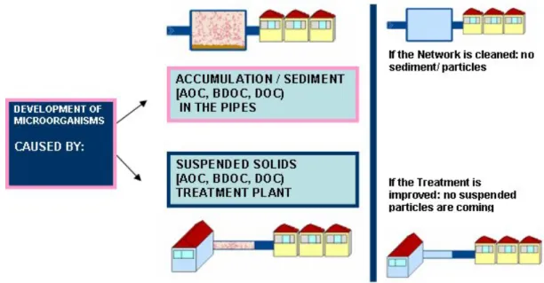
The hypothetic development of bacterial regrowth in the network is caused by:

1. Accumulation of sediment in the pipes (AOC, BDOC and DOC)

2. Suspended solids from the treatment plant (AOC, BDOC and DOC)

Fouling of drinking water system in relation to hydraulic circumstances and customer complaints 18

Fig. 2-2 Biological development under different cleaning frequencies and treatment standards

Regarding bacterial regrowth (see Fig. 2-2), the research hypotheses are:

1. Biological activity increases with higher temperatures;

2. Locations with high residence time are vulnerable to regrowth because of the transportation of sediments;

3. Changes in flow velocity affect the supply of substrates, biofilm sloughing and sediment accumulation;

3. Materials and Methods

The drinking water system is composed by the treatment plant, the transportation and distribution networks and the customers supply area. The treatment plant originates a certain amount of particles to the network and, within all of the particle-related processes, particles may settle, creating a layer of sediment, or resuspend, and a complaint may occur. In relation to biolfim regrowth, bacteria develop better if the amount of suspended solids and sediment is higher.

With the objective of studying the behaviour of particles at Oasen´s drinking water network, the following measurements were taken into account:

1. Turbidity at the major treatment plants (De Laak and Rodenhuis);

2. Resuspension potential measurements in the supply area of Rodenhuis and De Laak;

3. Complaints registration;

4. Aeromonas at the distribution and transportation pipes.

Turbidity, resuspension potential measurements and complaints registration are related to the discolouration risk, while Aeromonas relate to bacterial regrowth studies.

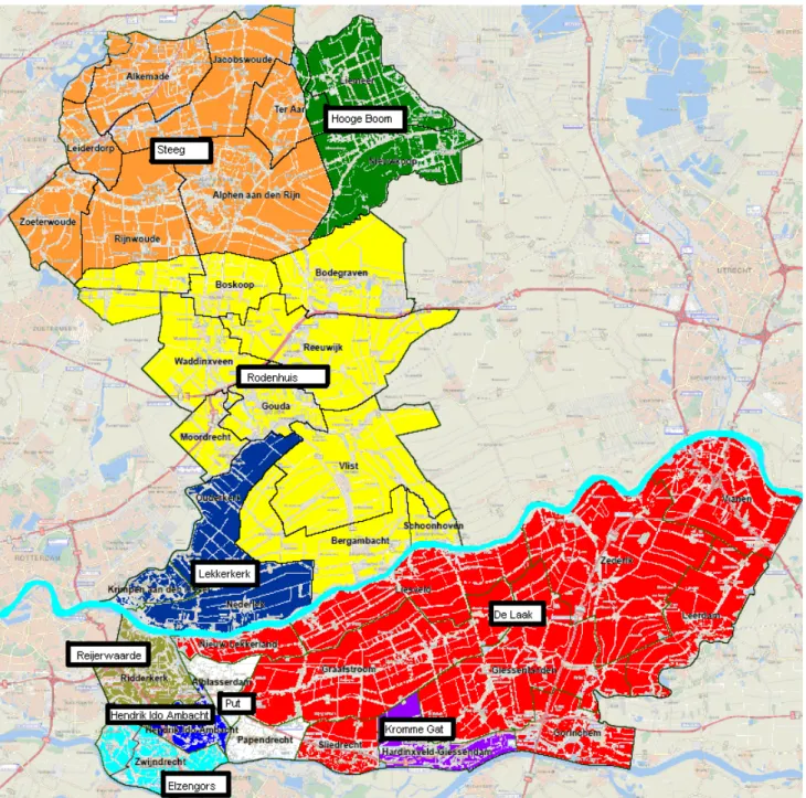
This study was developed at the Oasen’s supply area, located in the province of the South of Holland. Oasen’s distribution area is divided by the Lek River into north and south. The water is taken from groundwater riverbanks and there are ten treatment plants. These treatment plants have different supply areas and the major treatment plants are De Laak and Rodenhuis. De Laak is located in the south of the network and Rodenhuis in the North. The distribution network has around 300 000 connections and 700 000 inhabitants.

3.1 Turbidity measurements

Turbidity is measured online at the transportation area with Dr Lange Ultratub turbidimeters. The sampling frequency is every five minutes and measurements are hourly results based on averaging the five minutes results. The accuracy of the equipment is ±0,008 FTU and the minimum and maximum scales are 0,001 and 1000 FTU, respectively.

The threshold for turbidity accepted by the Dutch Law is 1 FTU at the treatment plant and 4 FTU at the consumers tap. The accepted threshold for Oasen is 0,1 FTU at the treatment plant. An example of online turbidity measuring at the transportation area is given in Fig. 3-2, where the thresholds of 0,1 FTU and 1 FTU are represented by an orange dot line.

Fig. 3-2 Example of online turbidity in an every-hour basis at Rodenhuis and De Laak (01-07-2007 to 22-08-2007)

Fouling of drinking water system in relation to hydraulic circumstances and customer complaints 22

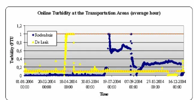
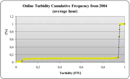
Online Turbidity Cumulative Frequency from 2004 (average hour) 0 0,2 0,4 0,6 0,8 1 1,2

0 0,2 0,4 0,6 0,8 1

Turbidity [FTU] P e r c e n ti le [ % ]

Fig. 3-3 Cumulative frequency distribution based on measured average hour online turbidity at De Laak´s transportation area (from 01-01-2004 till 31-12-2004).

The cumulative frequency distribution shows more variation where there is a shallow inclination than when the slope gets steeper and shifts to the left. Therefore, cumulative frequency shows how irregular the pattern is. Irregularity in the pattern may increase the discolouration risk, rather than a larger amount of particles.

The previous figures show the online turbidity for the average hour at De Laak in 2004 and the average turbidity at De Laak in 20047. The cumulative frequency from the graph (Fig. 3-3) was calculated from the average hourly turbidity from Fig. 3- 4. Since online turbidity is measured every five minutes, these results are the average of all every five minute averages within one hour.

From the cumulative frequency it is possible to say that the ratio between the higher percentile values is an indication of the shape and steepness of the curve. Through a simple calculation (see equations 1 and 2), from the Surface-90% and Surface+90%, we can identify a pattern as being more or less stable. The Surf-90% gives the ratio between the average value for turbidity below the 90-percentile measurement and the average for the whole period. The Surf+90% is the ratio above the 90-percentile and the total average.

Equations 3. 1 and 3.2

0-90 0-100

90-100 0-100

- 90% 0,9* *100%

90% 0,1* *100%

Average Surface Average Average Surface Average   

3.2 Resuspension potential method

The sediment analyses are performed using the Resuspension Potential Method (RPM). The method is based on the phenomenon of resuspending particles caused by a hydraulic disturbance [Vreeburg, 2007]. The hydraulic disturbance is achieved with the increase in velocity around 0,35 m/s and the method was developed in order to be applied in distribution pipes with diameters within 50 and 200 mm. The hydraulic shear stress of velocity causes the mobilisation of particles and affects the turbidity of the water. In this way, the RPM consists of a controlled and reproducible increase in the velocity within a pipe, aiming the measurement of the reactive turbidity to the hydraulic disturbance. The score is ranked and

Fouling of drinking water system in relation to hydraulic circumstances and customer complaints 24 translated into a Resuspension Potential result, with an obvious relation to the discoloration risk but not necessarily to the discolouration events. An increase of 0,35 m/s was determined [Vreeburg et al. 2004a] in the velocity measured from a pipe failure or fire hydrant. The turbidimeters used for the RPM can be the Sigrist KT65, which determines values at a dedicated measuring point, or Dr Lange Ultratub, which determines values at a flushing point. The standard method for the application of the Resuspension Potential Method is the following [Vreeburg, 2007] (Fig. 3-5):

 Isolate the pipe for which the discolouration risk is to be assessed, as for uni-directional flushing [Antoun et al. 1999]. The isolated length should be at least 315 meters long to be sure that only this single pipe is affected by the 15 minutes disturbance at 0,35 m/s;

 Open a fire hydrant so that the velocity in the pipe is increased by the additional

0,35 m/s above normal velocity and maintain that rate for fifteen minutes; afterwards reduce the flow to normal (total length affected is thus 315 m)

 Monitor turbidity in the pipe throughout the fifteen minutes of extra velocity and

beyond that until turbidity returns to the initial level.

The application of the method results in a graph:

Fig. 3-6 Typical RPM turbidity trace resulting from an RPM test (showing the four regions used to rate the discolouration risk) [Vreeburg, 2007].

From this picture, four regions can be used to trace the rank of the discolouration risk [Vreeburg, 2007]:

1. Base turbidity level

2. Initial increase in turbidity at the start of the hydraulic disturbance

3. Development of turbidity during the hydraulic disturbance

4. Resettling time and pattern to base (initial) turbidity level

Fouling of drinking water system in relation to hydraulic circumstances and customer complaints 26  The absolute maximum value of turbidity during the first five minutes of disturbance;

 The average value of turbidity during the first five minutes of disturbance;

 The absolute maximum value of turbidity during the last ten minutes of disturbance;

 The average value of turbidity during the last ten minutes of disturbance;

 The time needed to resettle again to the initial turbidity level.

The turbidity during the first five minutes represents the effect of resuspending sediment. Turbidity during the last ten minutes is the effect of a longer disturbance and can be lower than the initial acceleration effect. The resettling time makes it possible to determine where an increased level of turbidity is present, and can be notice by customers. The figure below is

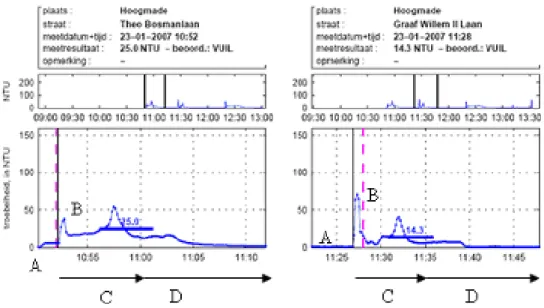
used to example of monitoring RPM at Jacobswoude in 2006.

Fig 3-7 Example of RPM measurements done in Jacobswoude (the base level (A), maximum level (B), disturbance time (C) and resettling me (D)).

Fig. 3- 8Typical RPM turbidity traces (before changing the average rank (A) and after changing the average rank 2005 (B)).

In relation to the chosen average, Oasen chooses the average for the RPM result from the 4th till the 9th minutes, instead of the last five minutes of disturbance. The main reason why Oasen changed the disturbance time is the shorter pipes´ lengths, which are 210 meters. In spite of, the water inside the pipes can be mixed with the water outside the measurements´

area, which results in a change in the average from the last five minutes to the 4th-9th range.

When comparing results determined in 2004 (before the chosen average changed) and 2005,

the difference is not significant. After opening the hydrant, the flow is often too high and needs to be adjusted, resulting in uncontrolled resuspension. Using velocity plates it is possible to avoid that resuspension and obtain more accurate results. The principle of the velocity plates states that a high resistance is created and the volume is restricted to a certain value, making it possible to open the hydrant and rapidly increase the flow up to the desired value.

Fouling of drinking water system in relation to hydraulic circumstances and customer complaints 28

Fig. 3-9 Average turbidity for the 4th-9th minute average: correct, overestimated and underestimated.

If the curve resembles the graph on the left, the average is suitable and no adaptations are needed. The chosen average can be from the last five minutes or from the 4th till the 9th minute. The maximum value should also be registered, as well as the resettling time.

If the average is overestimated, the RPM value is higher than it should and the discolouration risk is lower. The maximum value should be taken into account and the average should be adapted to the first five minutes of disturbance.

If the average turbidity is underestimated and the curve is similar to the graph on the right, the chosen average should be in the resettling time and the maximum value should be registered.

Instead of adapting all the curves, the threshold to start complaining can also be adapted. I suggest to use 20 FTU instead of 10 as the target to start cleaning the network.

The resettling time can be useful for the interpretation of the RPM graph, since it is the time needed for the discolouration risk, especially the complaint risk. If the time it takes turbidity to return to the base level is high, the risk of having a complaint increases.

Table 3-1 Example of ranking the RPM for discolouration using the Dr Lange Ultratub equipment at the flushing point [ Vreeburg, 2007]

0 1 2 3

Absolute max first 5 min. < 3 FTU 3 – 10 FTU 10 – 40 FTU > 40 FTU

Average first 5 min. < 3 FTU 3 – 10 FTU 10 – 40 FTU > 40 FTU

Absolute max last 5 min. < 3 FTU 3 – 10 FTU 10 – 40 FTU > 40 FTU

Average max last 5 min. < 3 FTU 3 – 10 FTU 10 – 40 FTU > 40 FTU

Time to clear < 5 min. 5-15 min. 15-60 min. > 60 min.

If the time needed to clear is less than 5 minutes, the discolouration risk is low; if it is between 5 and 15 minutes the sediment load is achieving the discolouration threshold to start complaining (10 FTU); and if it is between 15 and 30 minutes, the chance of having a complaint is high. In the practical application, the resettling time is often limited to 30

minutes.

Since a complaint may happen when turbidity reaches 10 FTU (whereas there is a large amount of sediment and a hydraulic disturbance) the selected boundaries for the interpretation of the RPM results are presented in Table 3-2.

Table 3-2 Boundaries for the rank of the discolouration risk in the pipes from the RPM

Average turbidity 4th-9th minute < 5 FTU/NTU Low discolouration risk

Average turbidity 4th-9th minute 5-10 FTU/NTU Medium discolouration risk

Average turbidity 4th-9th minute > 10 FTU/NTU High discolouration risk

As shown in the previous table, when the RPM results are below 5 FTU the discolouration risk is low to clean the network. If the RPM is between 5 and 10 FTU, the amount of sediment is reasonable and the discolouration risk should be overseen, regarding network cleaning in the early future. When the RPM result is higher than 10 FTU, there is a high discolouration risk.

Fouling of drinking water system in relation to hydraulic circumstances and customer complaints 30 3.3 Complaints´ Registration

A discoloured water complaint can happen when there is a hydraulic disturbance and a large amount of sediment. At Oasen, complaints registration uses the Accent Programme, where each client has a number and complaints are stored depending on customer’s observations. Technical complaints are the total number of complaints referring to water quality (different colour, discoloured water, presence of particles or invertebrates, softening or taste/odour).

The technical complaints process is demonstrated below.

Fig. 3-10 Process for the registration of a technical complaint at Oasen

If there is a problem regarding water quality, the customer may reach the company via telephone, internet, letter or personally. Based on the customer’s observations, a form is filled and the type and location of the problem are registered, including Date, Complaint Number, Type, Description, Street, House Number, Postal Code, City and Observations. After full filling all these parameters, the person in charge of solving the problem is selected and the duration of the complaint is registered (the time between receiving the call and solving the problem).

The type of complaint can be correlated with different colour (white water), discoloured water, presence of particles or invertebrates, softening or taste/odour. If there are more complaints on the same subject that means priority case, and registration refers the number of complaints, sending someone to solve the problem. The company says that all complaints are registered under the same procedure since 1999, even if the problem is general or if Oasen is already taking care of the situation.

1.Customer

- Telephone [website, digital phonebook, physical phonebook)

- Internet - Letter

- Personal communication

Registration in the Accent Programme.

Responsible person to check the problem

[for more than 1 complaint) 2.Oasen

Registration, cause and duration.

The same procedure is taken outside office hours, a call centre taking all the calls and registering remarks. If there is a priority call, Oasen is informed. In the end of the year, complaints registration calculates the number of complaints per 10 000 inhabitants per municipality. In order to judge the highness of the number of complaints, table 3-3 shows the thresholds I have calculated in order to have boundaries for the number of complaints.

Table 3-3 Threshold for discoloured water complaints and technical complaints in total (these thresholds were used for this thesis and applied for Oasen)

Number of discoloured water complaints > 2 / 10000 inhabitants

Total number of technical complaints > 4 / 10000 inhabitants

These thresholds were calculated using the number of customer complaints in relation to the number of connections, which is, from literature, 1 complaint per 1000 connections. The averaged number of discoloured water complaints is around 50% of the total number of technical complaints. Therefore it is assumed that discoloured water complaints are half of the total number of technical complaints. The calculation of the thresholds considered in Table 3-3 is based in the following equation:

*

int / 10 000 tan *10000

1 / 1000 (1 int / 1000 )

tan

A C Number of technical compla s inhabi ts

I

A compla connections

C number of connections I number of inhabi ts



  

Equation 3- 3

In Oasen the number of connections is around 300 000 and the number of inhabitants about 700 000, resulting in 4,3 technical complaints / 10 000 inhabitants and 2,15 discoloured water complaints / 10 000 inhabitants. For the guarantee of confidence, the thresholds were taken into the bottom integer.

Fouling of drinking water system in relation to hydraulic circumstances and customer complaints 32 this study refers only to discoloured water, only technical and discoloured water complaints were taken into account.

3.4 Bacterial regrowth

Bacterial regrowth is affected by many different factors, such as the concentration of the residual bacteria leaving the treatment plant, water temperature, disinfectant concentration8, sediment in the pipes, type/amount of nutrients and flow velocity [J. Bartram, et al. WHO 2003]. The key-parameters in this study are water temperature, flow velocity and residence time.

Aeromonasmeasurements took place in 2006 and 2007. Samples were taken by the company at the consumers tap and sent to the Vitens Laboratorium in Utrecht for analysis. Temperature is measured at the tap with a thermometer, after keeping the water running for 1 minute. Residence time and velocity are calculated with Alleid Programme for a demand situation of an average weekday. Transportation and distribution pipes have different residence time and flow velocity, which is reflected in bacteria concentration. Transportation pipes have diameters higher than 250mm. The considered threshold for the Aeromonas concentration is 1000 HPC / 100 ml. In order to prevent concentrations above that level, Oasen established 500 HPC / 100 ml as the limit concentration. When Aeromonas concentrations achieve this

value, they are considered “hotspots” (see Fig. 3-11).

8

Fouling of drinking water system in relation to hydraulic circumstances and customer complaints 34

4. Results

Measurements regarding the discolouration risk are turbidity at the treatment plant, RPM at the distribution area and the number of discoloured water complaints. The general idea to understand the discolouration risk was to cross the results from the RPM measurements and the number of complaints with treatment upgrading or network cleaning. Therefore, two supply areas with different characteristics were chosen and its results discussed.

In order to understand bacteria development in the network, measurements of potentially opportunistic pathogens, such as Aeromonas, were taken into account. The main factors considered were temperature, flow velocity and residence time.

4.1 Turbidity measurements

Turbidity is measured online at the treatment plants. These measurements provide an idea of the amount of suspended solids incoming from the treatment plant. Cumulative frequency distributions are also calculated regarding the turbidity pattern stability. More stability means releasing fewer particles to the network, even if turbidity is higher.

Turbidity is measured with Dr Lange Turbidimeters with a sampling frequency of five minutes. The hourly results represent the average of all the five minutes sampling taken in one hour. From the online turbidity measured in 2004, 2005 and 2006 at the major treatment

plants, cumulative frequencies based on hourly turbidity results per year were calculated and are presented in Table 4-1.

Table 4-1 Cumulative frequency for turbidity at Rodenhuis and De Laak

Rodenhuis 2004 2005 2006

Surface -90 [%] 67,6 60,8 67,8

Surface +90 [%] 32,4 39,6 32,2

Average Turbidity (hourly basis) 0,10 0,01 0,02

De Laak 2004 2005 2006

Surface -90 [%] 88,7 92,6 88,0

Surface +90 [%] 10,8 7,4 12,1

Based on Table 4-1, De Laak has a more stable turbidity pattern than Rodenhuis, from the higher Surf-90. Therefore, De Laak releases fewer particles into the network than Rodenhuis. At De Laak treatment was improved in 2003, which made the peaks smoother and the particle load decrease significantly.

The target value by the Dutch Law is 1 FTU and 0,1 FTU by Oasen, for turbidity at the treatment plant. Results from 2005 and 2006 are clearly beyond the limits. Next figure shows the average hourly turbidity per year from 1-1-2003 and 31-12-2004 at De Laak’s treatment plant.

Fig. 4- 1 Online monitoring of turbidity at De Laak (in 2003 (left) and 2004 (right)).

From the previous graph, it is possible to see a different pattern after the treatment changes (Dec-2003). Untill then, the graph is quite peaky, while in 2004 it resembles a bottom line. The peaks in 2003 are related to the filters backwashing. In 2004 softening, activated-carbon and UV disinfection were added to the treatment, so the flow peaks were absorbed and more particles were kept. Surface-90 at De Laak in 2003 is 79%, increasing to 88% after the treatment changed. Regarding the considered thresholds, before the treatment has changed, turbidity was higher than Oasen’s limit, while in 2004 turbidity was lower.

Fouling of drinking water system in relation to hydraulic circumstances and customer complaints 36 decreases the amount of suspended solids which settle at the distribution network, decreasing the discolouration risk.

At the locations with low turbidity and quite stable patterns (like Rodenhuis), the improvement in the treatment is not compulsory. However, if turbidity patterns get unstable or if average turbidity increases till the targets level, treatment upgrading should be considered.

4.2 Resuspension potential method

The RPM measurements are important for the discolouration risk analyses since they represent the amount of sediment that may lead to customer complaints. Moreover, if the RPM represent the amount of sediment in the network, when the network is cleaned and sediment is removed, the RPM results should decrease and so should the customer complaints. Given this, RPM measurements were plotted with customer complaints and cleaning frequencies to see correlations. The criterion to accept a linear correlation in this thesis is 0,70 as the minimum limit for the squared r. From Appendix 2 it is possible to see that the RPM measurements showed a big variation and no correlations could be found.

Since no correlations were found within all measurements, locations under the same conditions9were zoomed in and the expected correlations calculated (see Appendix 3). Again, no correlations could be found. So the effects on RPM and in the number of customer

complaints of cleaning the network or improving treatment were overseen. These effects are discussed in this section.

The zoomed locations were Rodenhuis and De Laak for being the major treatment plants. Rodenhuis is the reference area, where no treatment was improved and no cleanup performed and so a continuous increase in the amount of sediment through time (RPM measurements) was expected. At De Laak treatment was improved before the RPM measurements started (2003) and the network was cleaned between 2004 and 2005. Therefore, it is expected to see the number of complaints dropping when changes in the network was performed.

Results from Rodenhuis are summarised in Table 4-2 and De Laak in Table 4-3.

9

Table 4-2 RPM measurements at Rodenhuis

Municipality Street 2004 2005 2006/2007 Material and

diameter

Bergambacht Kastanje 2,1 27,9 22,7 PVC 110

Boskoop Pippeling 31,8 40,9 60,6 HPE 160

Sprengerstraat 4,8 14,8 42,5 PVC 110

Gouda Ericalaan 13,2 5 2,4 PVC 110

Jacob van Lennepkade 3,9 17,9 57 GIJ 110

Persinjstraat 44,7 17 32,9 PVC+GIJ

Ruigenbrug 3,2 0,3 2,6 PVC 110

Troetslaan 1 6,1 14,6 PVC 110

Haastrecht Bernardlaan 7,4 3,5 11,2 PVC 110

Moordrecht Sluislaan 3 15 13,8 PVC 110

Stevenstraat 0,7 25,3 4,7 PVC 110

Reewijk Beatrixlaan 17,1 4,2 50,9 PVC 110

Hoek van Mesdag 3,2 5,2 9,7 PVC 110

Schoonhoven R. van Heutzstraat 59,3 8,8 26,4 AC 100

Stolwijk Snippendreef 48,7 3,5 2,1 PVC 110

Vlist Berhardstraat 85,4 36,4 1,4 PVC/HPE 110

Waddinxveen Meidoonstraat 1,6 11,2 8,4 GIJ 118

st dev 25,4 12,1 20,2

average 19,5 14,3 21,4

Fouling of drinking water system in relation to hydraulic circumstances and customer complaints 38

Table 4-3 RPM measurements at De Laak

Municipality Street 2005 before cleaning 2005 after cleaning 2006/2007 Material and diameter

Liesveld Dorpstraat 1,3 1 0,5 *

Burgemester Viezlaan 1,7 1,8 60,4 *

Lijsterstraat 3,8 2,4 6,1 *

Reigerstraat 45,8 2 9,3 *

Liesdel 1,6 1,5 0,6 *

Van den Boetzlaerlaan 4,9 0,5 0,3 *

Graafstrom Pr. Willem Alenxandst. 21,9 1,3 15 *

Dorpstraat 73,5 1,8 13,6 *

Van Tielemanstraat 1,9 2,3 80,7 *

Peppelstraat 1,1 1,3 10,7 *

Gorinchem de Pauwstraat 17,7 1,9 40,2 GIJ 100

Kalkhaven 3,3 1,3 11,2 PVC 110

Jip em Janneke 1,4 1,7 3 PVC 110

Zederik Kastanjehof 4,3 0,4 5,1 *

Rijskade 1,5 4,6 2 *

Mr Haafkenstraat 5,8 9,7 16,6 *

Lijsterbeslaan 5,6 0,5 13,8 *

Mkillesteijinstraat 1,5 0,3 15,1 *

Hoogstraat 3,8 3 4,2 *

Zalingstraat 1,6 0,2 2,8 *

Giessenlanden Beatrizstraat 13,1 2 28,5 *

Perendreef 29,5 1,5 0,9 *

Bogerd 15,5 2,1 10,5 PVC 160

Maslostraat 5,6 2,8 5,9 PVC 160

Korenbloemstraat 40,5 2,1 3,1 *

De Schaus 1,5 3,2 4,8 *

JA van Vurenstraat 3,8 1,6 0,4 *

st dev 17,0 2,0 25,1

average 11,7 2,2 16,7

n 28

* There is no information on the pipe material and diameter for these measurements

Fig. 4-2 RPM, cleaning frequency (YAC = averaged number of years after the last cleaning was performed) and number of discoloured water complaints at Rodenhuis ( together with the error bars for standard deviation).

Fig. 4-3 RPM, cleaning frequency (YAC = number of years after the last cleaning was performed) and number of discoloured water complaints at De Laak (together with the error bars for standard deviation).

Rodenhuis -40 -30 -20 -10 0 10 20 30 40 50 60 70 80 90 100 110 120 130 140 150 A v er a g e R P M 0 1 2 3 A v er a g e n u m b e ro f co m p la in ts

RPM 56 15 16

YAC 12 14 15

C omplaints 1,88 2,64 1,30

2004 2005 2006

De Laak

-20 -10 0 10 20 30 40 50 A v er a g e R P M 0 5 10 15 20 25 A v er a g e n u m b er o f co m p la in ts

YAC 10,46 0,25 1,50

RPM 18 2 12

Complaints 21,56 1,77 0,38

Fouling of drinking water system in relation to hydraulic circumstances and customer complaints 40 From Fig. 4-2, RPM dropped from the first to the second measurement, instead of decreasing through the all period, as originally expected. The reason for this to happen is that measurements may have acted like network cleaners themselves, removing the major part of the sediment in the pipes. Since the RPM reached equilibrium from 2005 to 2006 and the turbidity average is quite low at Rodenhuis (Table 4-1), the recharging from the treatment plant is slow, especially if RPM measurements keep managing the sediment in the network by themselves. If the number of particles coming from the treatment plant does not increase and RPM measurements stop: sediment should slowly reach an RPM level around the initial value of 50 FTU. If the number of particles coming from the treatment plant does not increase and RPM measurements continue: sediment continues being managed by the measurements themselves and should stay around 15 – 20 FTU. The number of customer complaints at this treatment plant is below the threshold of 2 discoloured water complaints / 10 000 inhabitants both in 2004 and 2006 and it is slightly higher than that limit in 2005. The increase in the number of complaints from 2004 to 2005 was probably caused by the activity associated to the measurements themselves.

At the Laak (Fig. 4-3), the effect of cleaning the network can be clearly identified with the drop in the RPM and in the number of complaints from 2004 to 2005 (the network was cleaned in between). However, from 2005 to 2006, RPM increases till the initial level,

suggesting rapid sediment regeneration. Hence, either the RPM is not measuring the actual discolouration risk or the method of cleaning the network is not enough for long-term analysis

or the threshold to start complaining is not adjusted to the local circumstances. Checking the increase in the standard deviation from 2005 to 2006, the cleaning frequency is around 6 and 12 months. Regarding the number of complaints in De Laak, it decreases considerably since the network cleaning and continues dropping until 2006. These results lead to the conclusion: the RPM is not related to the customer complaints. Although, the number of complaints in 2004 is possibly higher because of the treatment changes (which started in December 2003 and ended in May 2004), and in 2005 for the activity associated to the measurements themselves.

leading to RPM values between 10 and 20 FTU and a low level of customer complaints. From these results, the threshold to start complaining should be higher. The threshold of 20 FTU can be suggested for performing a network cleanup. Although, regarding the standard deviation for the RPM other cleaning methods, such as unidirectional flushing could be studied.

4.3 Complaints registration

The discolouration risk analyses exist to prevent the customers from complaining. After analysing the suspended solids coming from the treatment plant (online turbidity) and the RPM in the pipes (RPM), the customers experience shall be discussed. The accepted thresholds are 2 for the number of discoloured water complaints per 10 000 inhabitants per year and 4 for the number of technical complaints per 10 000 inhabitants per year. Technical complaints refer to water quality in general and discoloured water complaints to the brown water phenomena, and these are the main contributors for the total number of technical complaints (around 50%). The absolute numbers of discoloured water and technical complaints are presented in Fig. 4-4.

Fouling of drinking water system in relation to hydraulic circumstances and customer complaints 42 The table below shows the number of technical and discoloured water complaints per 10 000 inhabitants per year.

Table 4-4 Number of complaints per 10 000 inhabitants

Year Technical Complaints Discoloured Water

2000 4,40 2,48

2001 4,74 2,94

2002 6,10 4,07

2003 6,03 4,26

2004 4,49 2,48

2005 4,00 1,68

2006 3,00 1,33

From Fig. 4-4, discoloured water complaints are representative of the behaviour of technical complaints. From Table 4-4, the number of discoloured water and technical complaints are below the considered thresholds only in 2005 and 2006. The number of complaints of 2006 per 10 000 inhabitants at every treatment plant and the average for overall years from 1999 till 2006 are summarised in Table 4-5. Results from the five major treatment plants are plotted in the next figure.

Table 4-5 Number of complaints per 10 000 inhabitants at each treatment plant (from 1999 till 2006)

Treatment Plant Discoloured water 2006 Discoloured water total 1999-2006 Number of inhabitants Level/

2006 Average / year

Put 1 20 49296 0,2 0,5

Steeg 3 250 93482 0,3 3,3

Rodenhuis 8 197 185154 0,4 1,3

De Laak 8 916 145611 0,6 7,9

Kromme Gat 4 46 17812 2,5 3,2

Hendrik Ido Ambacht 1 4 22959 0,4 0,2

Lekkerkerk 0 1 14833 0,0 0,1

Hooge Boom 17 287 17807 9,6 20,1

Reijerwaarde 0 9 45534 0,0 0,2

Elzengors 0 3 41719 0,1 0,1

Fig. 4-5 Performed cleaning activities (at De Steeg (#1 and #2), Rodenhuis (#1) and at De Laak (#4)) and treatment improvements (at De Laak (#3) in relation to the number of discoloured water complaints per 10 000 inhabitants (1999-2009). In the vertical axis we have the number of customer complaints/10 000 inhabitants and in the horizontal axis the timeline.

Applying the threshold for the number of discoloured water complaints, the Steeg, De Laak

and Hooge Boom are the most problematic treatment plants during the entire period, while Kromme Gat and Hooge Boom have the highest values in 2006. At these treatment plants, turbidity patterns and RPM measurements should be analysed, in order to see if the network needs some cleanup or if treatment needs to be improved. Regarding the number of discoloured water complaints at each treatment plant (Fig. 4-5), the effects of cleaning the network and improving treatment can be seen from the decrease in the number of complaints. However, there are supply areas where no changes were performed and where the number of complaints decreases significantly, like Hooge Boom and Kromme Gat. Oasen says there were repairs in the network and maintenance works, which may justify the peak in 2002.

As a remark, the fact that cleaning was performed at one treatment supply area does not mean that all of the whole supply area was cleaned, like in Rodenhuis.

0 10 20 30 40 50 60 70 80 90 100

1999 2000 2001 2002 2003 2004 2005 2006 Average all complaints Hooge Boom Kromme Gat De Laak Rodenhuis Steeg

Fouling of drinking water system in relation to hydraulic circumstances and customer complaints 44 Zooming in the previous figure, it is possible to analyze the effect of improving the treatment in 2003 and cleaning the network in 2005 at De Laak, from the number of complaints (y axis) (see next figure).

Fig. 4-6 Effects of improving treatment (2003) and cleaning the network (2005) at De Laak (orange line). In the vertical axis we have the number of customer complaints/10 000 inhabitants and in the horizontal axis the timeline.

4.4 Results of the bacterial regrowth

The analysed parameters regarding bacterial regrowth are: water temperature, calculated residence time and flow velocity. From these measurements, mathematical correlations were sought and Aeromonas variation with each parameter was exploited. Bacteria concentrations were also divided into “hotspots”, for higher concentrations than the Oasen’s target level (500 HPC/ml), and “non-hotspot”, if the concentration stays below that level. Measurements were done in 2006 and 2007, but by the time this thesis was written, only residence times and flow velocity calculations from 2006 were available. Measurements with concentrations equal to 9999 HPC/100 ml were not considered, for they are not representative.

4.4.1 Aeromonas and water temperature

Water temperature is the classical parameter related to microbial activity. Since the goal of this study is to know how to control bacterial regrowth, for the temperature analyses, only concentrations above the target level of 500 HPC/100 ml were taken into account. Therefore, bacterial concentrations were divided into percentage of hotspots and percentage of non-hotspots from 2006 (cold summer) and 2007 (warm summer) (see next table).

Table 4-6 Percentage of hotspots (from a hot summer (2006) and a cold summer (2007))

% Hotspots in a hot summer (year: 2006) 29%

Average temperature (°C)

18.0

Number of measurements 356

% Hotspots in a cold summer (year: 2007)

16%

Average temperature (°C) 17.4

Number of measurements

55

Fouling of drinking water system in relation to hydraulic circumstances and customer complaints 46

Table 4-7 Percentage of hotspots and temperature (2006)

Temperature of the water (°C)

13 14 15 16 17 18 19 20 21 22 23 24 25 27

% Hotspots 0% 12% 5% 0% 19% 25% 25% 40% 50% 67% 69% 33% 25% 100%

N 1 8 21 26 44 56 76 50 26 18 16 9 4 1

Fig. 4-7 Percentage of hotspots and temperature (in July and August (2006))

This figure shows that water temperature and bacterial regrowth are correlated and the optimal temperature for the Aeromonas regrowth is around 22 or 23 degrees.

After analysing the measurements, three temperature classes can be ranged:

 Low temperatures (13 – 17 °C): 10% of the measurements are hotspots

 Middle temperatures (18 – 20 °C): 30% of the measurements are hotspots

Since July and August are the warmer months and 2006 was a hot summer, these results may work for the worst case scenario.

4.4.2 Aeromonas and residence time

Locations with high residence times are vulnerable to regrowth. The figure below shows the variation of Aeromonas concentration with residence time for all the temperature ranges.

Fig. 4-8 Aeromonas and residence time (from 2006)

From the squared r there is no mathematical correlation between Aeromonas and residence time. However, below 20 hours the number of hotspots is quite low and below 10 hours there are no hotspots. Since no mathematical correlation was found within all the temperature ranges, measurements were separated in three temperature classes. The variation of

Fouling of drinking water system in relation to hydraulic circumstances and customer complaints 48

Fig. 4-9 Aeromonas and residence time between 13 and 17 ºC

Therefore, within this temperature range, residence time is correlated with bacterial development. In Appendix 6 it is possible to see the Aeromonas variation within 18 -27 °C.

4.4.3 Aeromonas and flow velocity

Fig. 4-10 Aeromonas and flow velocity ( from July and August 2006)

Fouling of drinking water system in relation to hydraulic circumstances and customer complaints 50

Fig. 4-11 Aeromonas and flow velocity within 18 and 20 ºC

5. Case-study: cast-iron and non cast-iron networks

5.1 Introduction

Discoloured water is caused by the resuspension of deposited materials as a result of velocity increase. The materials origins can be the treatment plant or the corrosion of unprotected cast-iron or steel mains.

Previous studies concluded that cast-iron networks are not the major cause for discolouration [Vreeburg, 2007], [Smith et al, 1997: McNeil and Edwards, 2001], pointing the treatment plant as the most important source of particles. In this case-study, the goal was to investigate if cast-iron networks release more particles into the network than PVC networks, based on RPM results.

In this chapter, an Oasen’s RPM interpretation is also discussed.

5.2 Materials and methods

The research area was Leiderdorp, supplied by De Steeg treatment plant. In total, eleven measuring points were selected (Fig. 5-1), of which only eight could be measured due to the inaccessibility of a few hydrants10. Therefore, in Fig. 5-1, measurements #2, #4 and #9 are missing.

The research area is divided into cast-iron pipes (red coloured pipes in Fig. 5-1) and PVC pipes (yellow coloured pipes in Fig. 5-1). The cast-iron diameter is 98 mm and the PVC diameter is 110 mm. The cast-iron pipes were built in 1950, while the PVC pipes were built in 1998.

Fouling of drinking water system in relation to hydraulic circumstances and customer complaints 52

Fig. 5-1 Monitoring cast-iron and PVC networks (Leiderdorp, 10-10-2007)

5.3 Results

The maximum and the minimum results obtained from the turbidity average of the 4th-9th range for the cast-iron networks are presented below.

Fig. 5-3 Maximum (on the left) and minimum (on the right) RPM scores from the cast-iron pipes (16-10-2007)

The analysed cast-iron networks have a very high turbidity average (149 FTU), considering

the threshold to start complaining 10 FTU. Looking into the RPM in the graph on the right, the chosen RPM average is suitable. Checking out the resettling time, turbidity does not reach the initial base level after the 10 minutes period of disturbance. The resettling time is over ten minutes.

Fouling of drinking water system in relation to hydraulic circumstances and customer complaints 54

Fig. 5-4 Maximum and minimum RPM scores from the PVC pipes (16-10-2007)

The analysed PVC networks have a high turbidity average (19 FTU), considering the threshold to start complaining (10 FTU). However, results obtained from PVC networks are much lower than the cast-iron results. From these measurements, the discolouration risk is higher for the cast-iron, meaning more particles added to the system. Looking into the RPM curves, the resettling time should be around ten minutes for both experiments, since the turbidity level is around the initial baseline when measurements stop. The average turbidity from the RPM graph on the right side, the RPM is underestimated. Despite, the graph bellow shows an example of RPM adjustment.

The real turbidity average should be about 40 FTU, higher than the previous value of 22 FTU. The complete results from the RPM measurements are presented in Appendix 8. The figures bellow show the water coming out from a cast-iron pipe and from a PVC pipe.

Fig. 5-6 Brown water coming out of the cast-iron pipes (on the left) and clear water from PVC (on the right)

The pictures lead us to believe that cast-iron realeses much more particles than PVC.

5.4 Discussion

From the previous measurements, cast-iron networks have a higher discolouration risk than PVC networks. A few considerations should, however, be taken into account:

 The cast-iron pipes roughness may accumulate more sediment, which can be easily

resuspended;

 The smaller diameters from the cast-iron pipes may increase flow velocity, creating more sediment that can also resuspend. This can be evaluated by means of pressure drop calculations;

 The cast-iron pipes were built in 1950 while the PVC pipes were built in 1998.

Fouling of drinking water system in relation to hydraulic circumstances and customer complaints 56 5.5 Conclusion

Cast-iron measurements have higher and larger peaks than non cast-iron measurements, meaning a higher discolouration risk. However, to conclude that cast-iron pipes contribute with more sediment to the network, further measurements including sediment-analysis and pressure drop should be performed.

6. Conclusions

6.1 Discolouration risk

 If water quality improves, less particles enter the network and the discolouration risk decreases.

The effect of particles in drinking water systems can be observed from turbidity analyses. Turbidity cumulative frequencies used together with the average values, the percentile ratios

and the Surf+90 and Surf-90, make it possible to compare particle loads from different treatment plants. As shown in Fig 3-1, the treatment’s improvement in the end of 2003 increases the patterns stability making the turbidity peaks smother, which reduces the number of particles in the network and declines the discolouration risk.

 When cleaning is performed and sediment is removed, the discolouration risk decreases.

The RPM is related to the discolouration risk because measurements relate to the resuspension of particles by increasing flow velocity. Measuring the RPM pre and post cleaning, it is possible to evaluate the cleaning performance. The RPM results are used to measure the critical level of accumulation of sediment in the network and the efficiency of the cleaning method. From Fig. 3-3, when cleaning is effective in removing the sediment, the discolouration risk decreases.

 If the discolouration risk decreases, it is reflected in the number of discoloured water

complaints.

Discoloured water complaints can be used as an effect-measuring tool of discolouration risk. The measuring of the discolouration risk with RPM (Figures 3-2 and 3-3) indicates that when the RPM results decrease the number of complaints decreases as well.

 When treatment is improved, the cleaning frequency is lower.