doi: 10.1590/0101-7438.2015.035.03.0555
A DISTRIBUTION FOR THE SERVICE MODEL
Silvia Maria Prado
1*, Francisco Louzada
2,
Jos´e Gilberto S. Rinaldi
3and Benedito Galv˜ao Benze
4Received June 30, 2014 / Accepted September 3, 2015
ABSTRACT.In this paper, we propose a distribution that describes a specific system. The system has a heavy traffic, a fast service and the service rate depends on state of the system. This distribution we call the Maximum-Conway-Maxwell-Poisson-exponential distribution, denoted by MAXCOMPE distribution. The MAXCOMPE distribution is obtained by compound distributions in which we use the zero truncated Conway-Maxwell-Poisson distribution and the exponential distribution. This distribution has adjustment mechanism in order to re-establish the equilibrium of the system when the traffic flow increases and that is described by variations of the pressure parameter. Because of this, the MAXCOMPE distribution contains sub-models, such as, the Maximum-geometric-exponential distribution, the Maximum-Poisson-exponential distribution and the Maximum-Bernoulli-exponential distribution. The properties of the proposed distribu-tion are discussed, including formal proof of its density funcdistribu-tion and explicit algebraic formulas for their reliability function and moments. The parameter estimation is based on the usual maximum likelihood method. Simulated and real data are shown to illustrate the applicability of the model.
Keywords: MAXCOMPE distribution, service rate, server.
1 INTRODUCTION
In this paper, the studied system is very specific. The system has a single-server, fast service and heavy traffic. Furthermore, the service rate depends on state of the system, that is, when the num-ber of customers increases, the service rate increases. The arrivals of the customers in the system are attached to the service, in other words, when a service finishes, another customer arrives and he enters into service directly. Thus, the service time is the same as inter-arrival time. For this reason, this system has an adjustment mechanism in order to re-establish the equilibrium of the
*Corresponding author.
1Universidade Federal de Mato Grosso, Cuiab´a, MT, Brasil – E-mail: [email protected] 2Universidade de S˜ao Paulo, S˜ao Carlos, SP, Brasil – E-mail: [email protected]
system and avoid congestion. The increase in service rate and the opening the new service chan-nels are the adjustment mechanisms. Some examples of systems with this behavior are nonstop toll electronic, the traffic flow and the access on website.
We propose the Maximum-Conway-Maxwell-Poisson-exponential distribution, denoted by MAXCOMPE distribution to describe this system. Moreover, we are particularly interested on the maximum inter-arrival time or maximum service time. The methodology used to obtain this distribution is the compound distributions. We compose the zero truncated Conway-Maxwell-Poisson distribution and the exponential distribution.
The MAXCOMPE distribution contains sub-models that describe the variations of the system, such as, the Maximum-geometric-exponential distribution, denoted by MAXGE distribution, the Poisson-exponential distribution, denoted by MAXPE distribution and Maximum-Bernoulli-exponential distribution, denoted by MAXBE distribution.
The compound distributions has been extensively studied. We mention the following articles: Barreto-Souza et al. (2011) introduced the Weibull-geometric distribution which generalizes the exponential-geometric distribution proposed by Adamidis et al. (2005) and Cancho et al. (2011) proposed the Poisson-exponential distribution with two-parameters, Cordeiro et al. (2012) intro-duced a new three parameters distribution called exponential-Conway-Maxwell Poisson distri-bution, denoted by ECOMP distribution.
This paper is organized as follows. In Section 2, the MAXCOMPE distribution and some of its properties are presented. The expressions for the density function andr-th moment of the MAXCOMPE distribution are described. In Section 3, we discuss maximum likelihood estima-tion. In Section 4, some numerical results with simulation and real data are showed. Conclusions are presented in Section 5.
2 THE MAXCOMPE DISTRIBUTION
In this section, we present the MAXCOMPE distribution. Consider the arrivals of the customers occur at random, inter-arrival times are exponentially distributed with meanλ, the service time is exponentially distributed and its mean is dependent on the system state, given byµm =mφµ,
whereφis pressure parameter which indicates the degree that the service rate is affected by the state of the system,mis the number of customers in the system andµis the service rate. The service discipline is considered to be first-in-first-out (FIFO).
When the pressure parameter assumes the values zero,φ=0, the system is not accelerated and an adjustment is not required, forφ=1 the service rate is proportional to the state of the queuing system and the service channels are open, forφ → ∞the system is more accelerated and the service is very fast.
In Figure 1 we show the scheme of the system with the three variations of the pressure parameter.
Let M be a random variable representing the number of customers in the system with a zero truncated COMP distribution (Cordeiro et al., 2012). Its probability mass function is expressed as
P(M =m)= 1 [Z(ρ , φ)−1]
ρm
(m!)φ, m=1,2, . . . , (1)
where Z(ρ , φ)=∞j=0(ρj!j)φ is a normalizing constant,ρ > 0 is the traffic intensity andφ ∈
[∞,∞]is the pressure parameter.
Furthermore,φ ∈ [−∞,1)the work is not accelerated and the service center. Forφ ∈ (1,∞]
the work in the center is accelerated and some adjustments are needed. Forφ=0, we have the geometric distribution. Forφ=1, we have the Poisson distribution and forφ→ ∞we have the Bernoulli distribution.
Let Yi, i = 1,2, . . ., be independent random variables denoting the inter-arrival times. The
random variableYi is exponentially distributed with parameterλ >0 and its density function is
given by
fYi(yi;λ)=λe
−λyi, y
i >0. (2)
Consider the random variableY = max(Y1, . . .YM)that represents the maximum inter-arrival
time or the maximum service time.
In the following proposition, we provide the distribution that describes the studied system.
Proposition 1. Consider M, Y1,Y2, . . .independent random variables defined above. The den-sity function of the MAXCOMPE distribution is given by
fY(y;θ )=
1
[Z(ρ , φ)−1]ρλe
−λy
∞
m=1
m(ρ(1−e
−λy))m−1
(m!)φ , (3)
whereθ =(ρ , λ, φ)T is the vector of parameters,λ >0is the arrival rate,ρ <1is the traffic intensity andφ∈(−∞,∞)is the pressure parameter.
Proof. The conditional density function of theY givenM=mis provided by
fY(y|M =m;λ) = m fY1(y)(FY1(y))
m−1
= mλe−λy(1−e−λy)m−1,
where fY1(·)is the density function of theY1 andFY1(·)is the probability function of theY1.
Therefore, the density function of the MAXCOMPE distribution is given by
fY(y;θ) =
∞
m=1
P(M =m)fY(y|M =m;λ)
= 1
[Z(ρ , φ)−1]ρλe
−λy
∞
m=1
m(ρ(1−e−λy))m−1 (m!)φ .
The distribution function of the MAXCOMPE distribution is given by
FY(y;θ) =
1
[Z(ρ , φ)−1]
∞
m=1 m ρ
m
(m!)φ y
0
λe−λu(1−e−λu)m−1du
= 1
[Z(ρ , φ)−1]
∞
m=0
(ρ(1−e−λy))m (m!)φ −1
= Z(ρ(1−e
−λy), φ)−1
[Z(ρ , φ)−1] , (4)
whereZ(ρ(1−e−λy), φ)=∞ m=0
(ρ(1−e−λy))m (m!)φ .
The reliability function of the MAXCOMPE distribution is
WY(y;θ)=
Z(ρ , φ)−Z(ρ(1−e−λy), φ)
[Z(ρ , φ)−1] . (5)
Ther-th moment ofY is given by
E(Yr) = 1 [Z(ρ , φ)−1]
∞
m=1 mρm (m!)φ
∞
0
yrλe−λy(1−e−λy)m−1d y
= 1
[Z(ρ , φ)−1]
∞
m=1 mρm (m!)φ
m−1
k=0
(−1)k m−1
k
∞
0
yrλe−λye−kλyd y
=λ
−rŴ(r+1)ρ [Z(ρ , φ)−1]
∞
m=1 mρm (m!)φ
m−1
k=0
(−1)k m−1
k
1 (1+k)r
×
∞
0
yr(λ(1+k))e−λ(1+k)yd y
= λ
−rŴ(r+1) [Z(ρ , φ)−1]
∞
m=1 mρm (m!)φ
m−1
k=0
(−1)k m−1
k
1
(1+k)r. (6)
The Equation (6) can be calculated numerically by truncation (Gradshte˘ın et al., 2007). The truncation of this sum is described in Appendix.
The MAXCOMPE distribution has sub-models that are presented via the corollaries below.
Corollary 1.When the pressure parameterφassumes the value zero, the MAXCOMPE distribu-tion becomes the Maximum-geometric-exponential distribudistribu-tion, denoted by MAXGE distribudistribu-tion. The density function of the MAXGE distribution is
fY(y;ρ , λ)=
λe−λy(1−ρ)
(1−ρ(1−e−λy))2, (7)
In this case, the service rate is independent on state of the system.
The reliability function is given by
WY(y;ρ , λ)=
e−λy
(1−ρ(1−e−(λy)k
)). (8)
Ther-th moment ofY is given by
E(Yr)=(1−ρ)λ−rŴ(r+1)
∞
m=1 mρm
m−1
k=0
(−1)k m−1
k
1
(1+k)r, (9)
The sum in Equation (9) is truncated the same way that in the Equation (6) (see Appendix).
Corollary 2. When the pressure parameterφassumes the value one,φ=1, the MAXCOMPE distribution becomes the Maximum-Poisson-exponential distribution, denoted by MAXPE distri-bution. The density function of the MAXPE distribution is given by
fY(y;ρ , λ)=
ρλe−λy+ρ (1−e−λy)
(eρ−1) , (10)
whereλ >0andρ >0, in this case there is not restriction forρ.
The service rate is directly proportional to the state of the system. Furthermore, new service channels are opened.
The reliability function is given by
WY(y;ρ , λ)=
eρ−eρ (1−e−λy)
(eρ−1) . (11)
Ther-th moment ofY is given by
E(Yr)=λ
−rŴ(r+1) eρ−1
∞
m=1 mρm (m!)
m−1
k=0
(−1)k m−1
k
1
(1+k)r. (12)
The sum in Equation (12) is truncated the same way that in the Equation (6) (see Appendix)
Corollary 3. Whenφ → ∞, the MAXCOMPE distribution becomes the Maximum-Bernoulli-exponential distribution, denoted by MAXBE distribution. The density function of the MAXBE is given by
fY(y;λ)=λe−λy, (13)
whereλ >0.
The reliability function is given by
Ther-th moment ofY is given by
E(Yr)=λ−rŴ(r+1). (15)
3 MAXIMUM LIKELIHOOD ESTIMATION
Lety=(y1, . . . ,yn)be a random sample ofY which it has the MAXCOMPE distribution with
unknown parameter vector=(ρ , λ, φ)T. The log likelihood function foris
ℓ(θ) = −nlog[Z(ρ , φ)−1] +nlogλ−λ
n
i=1
yi+nlogρ
+ n
i=1
log
∞
m=1
m(ρ(1−e−λyi))m−1
(m!)φ
. (16)
The score functionU()=(Uρ,Uλ,Uφ)T has components
Uρ = − n [Z(ρ , φ)−1]
∞
m=1 mρm−1
(m!)φ + n
ρ +
n
i=1
∞
m=1
m(ρ(1−e−λyi))m−1
(m!)φ
−1
×
∞
m=1
m(m−1)ρm−2(1−e−λyi)m−1
(m!)φ , (17)
Uλ = n
λ−
n
i=1 yi +
n
i=1
∞
m=1
m(ρ(1−e−λyi))m−1
(m!)φ
−1
×
∞
m=1
m(m−1)ρm−1(1−e−λyi)m−2y
ie−λyi
(m!)φ , (18)
Uφ =
n [Z(ρ , φ)−1]
∞
m=1
ρmlog(m!) (m!)φ −
n
i=1
∞
m=1
m(ρ(1−e−λyi))m−1
(m!)φ
−1
×
∞
m=1
m(ρ(1−e−λyi))m−1log(m!)
(m!)φ . (19)
The maximum likelihood estimates (MLEs) ˆ of are obtained by solving the Equations
U() = 0. We use the numerical maximization byoptimpackage in software R (Rigby & Stasinopoulos, 2005).
Under some regularity conditions,ˆ has asymptotic multivariate normal distribution with mean and varianceI−1()),
I()=E
− ∂ 2ℓ
∂T
, (20)
whereI()is Fisher information matrix. Furthermore,
I()= − ∂ 2ℓ
∂T
is the observed Fisher information matrix. This result can be used to construct confidence inter-vals for the parameters of the distribution.
The log likelihood function for the sub-models are shown below.
• The log likelihood function of the MAXGE distribution is given by
ℓ(ρ , λ)=nlog(1−ρ)+nlogλ−λ
n
i=1 yi−2
n
i=1
log(1−ρ(1−e−λyi)). (21)
The components of the score function are given by
Uρ = − n
(1−ρ)+2
n
i=1
(1−e−λyi)
(1−ρ(1−e−λyi)), (22)
Uλ = n
λ−
n
i=1 yi+2ρ
n
i=1
yie−λyi
(1−ρ(1−e−λyi)). (23)
• The log likelihood function of the MAXPE distribution is
ℓ(ρ , λ)=nlogρ+nlogλ−λ
n
i=1
yi+nρ−ρ n
i=1
e−λyi −nlog(eρ−1). (24)
The components of the score function are given by
Uρ = n
ρ +n−
n
i=1
e−λyi − ne
ρ
(eρ −1), (25)
Uλ = n
λ−
n
i=1 yi+ρ
n
i=1
yie−λyi. (26)
• The log likelihood function of the MAXBE distribution is
ℓ(λ)=nlogλ−λ
n
i=1
yi. (27)
The score function is
Uλ= n
λ −
n
i=1
yi. (28)
4 NUMERICAL RESULTS
4.1 Simulation
The studied system was simulated by M/M/1 model. This model can be applied to provide approximate of other models (Whitt, 1989). We simulated twoM/M/1 models with two pairs of values(ρ , λ, φ): (0.8,0,8,0)and(0.9,0.9,0). These parameters were chosen because the system has heavy traffic, thus, withρ =0.8 and 0.9 the server has 80% and 90% of observed time occupied. We establish 10,000 arrivals in the system as the ending point of the simulation. The sample size in each simulation is 9.000 service times. We choose the simulations nearest of the studied system. In other words, the system with the queue that has the shortest length.
Therefore, the simulated models have single server, heavy traffic and the service rate indepen-dent on state of the system. Due to the fact, the MAXGE distribution was chosen to model the maximum service time.
In the Tables 1 and 2 we show the summary of the simulations chosen to represent the system. We observe that the standard-deviation increases when the traffic intensity increases.
Table 1–Summary of the simulated data withρ=0.8. Mean Median Maximum Minimum Standard-deviation
1.203 0.806 8.240 0.0033 1.272
Table 2–Summary of the simulated data withρ=0.9. Mean Median Maximum Minimum Standard-deviation
1.26 0.741 8.090 0.0002 1.488
The parameters of the model are estimated by maximum likelihood method. Numerical max-imization of the log likelihood function is accomplished by using the RS method (Rigby & Stasinopoulos, 2005). In Table 3 we show the MLEs of the MAXGE distribution, its to the re-spective confidence interval (CI) and standard error (sde).
Table 3–The MLEs, the confidence intervals (CI) 95% and sde for the parameters of the MAXGE distribution.
True Parameter ρˆ CI(95%) sde λˆ CI(95%) sde
ρ=0.8 0.801 (0.791,0.808) 0.0148 0.80 (0.795,0.804) 0.004
ρ=0.9 0.902 (0.890,0.907) 0.010 0.9 (0.895,0.909) 0.005
Table 4–Maximum likelihood simulation study of the MAXGE distribution forρ=0.8 andλ=0.8. True parameters:ρ=0.8,λ=0.8
Sample size n=50 n=250 n=500 n=700 n=1,000
ˆ
ρ λˆ ρˆ λˆ ρˆ λˆ ρˆ λˆ ρˆ λˆ
Sample mean 0.90 0.91 0.93 0.79 0.89 0.87 0.82 0.86 0.8 0.82
Variance 1.21 1.31 0.60 0.14 0.30 0.05 0.064 0.0026 0.009 0.0027
Bias -0.10 -0.11 -0.03 0.01 -0.09 -0.07 -0.02 -0.04 0 0.02
Table 5–Maximum likelihood simulation study of the MAXGE distribution forρ=0.9 andλ=0.9. True parameters:ρ=0.9,λ=0.9
Sample size n=50 n=250 n=500 n=700 n=1,000
ˆ
ρ λˆ ρˆ λˆ ρˆ λˆ ρˆ λˆ ρˆ λˆ
Sample mean 1.0 0.99 0.95 0.86 0.92 0.87 0.92 0.93 0.90 0.89 Variance 1.21 1.31 0.60 0.14 0.10 0.07 0.026 0.005 0.010 0.0023
Bias -0.1 -0.09 -0.05 0.04 -0.02 0.03 -0.02 -0.03 0 0.01
We can study the goodness of fit of the proposed model by the comparison between the observed and predicted values. The simplest way to make this comparison is graphically, which consists to compare the reliability function of the MAXGE distribution with the estimated reliability function by Kaplan-Meier method (Kaplan & Meier, 1958).
In the Figure 2 we compare the reliability function of the MAXGE distribution with the estimated reliability function. We observe that the reliability function of the MAXGE distribution has a close concordance with the estimated reliability function.
We use Log-rank and Chi-squared tests to evaluate if a closeness of the curves is significant or not (Kleinbaum & Klein, 2012 and Massey Jr, 1951). The null hypothesis of the tests cited is that there is no difference between the reliability functions.
We make 1,000 replications with different ending points to obtain the number of times that the null hypothesis is not rejected. The concordance percentages of the tests presented in Table 6 show that concordance increases as the traffic intensity, and ending point increases.
Table 6–Concordance percentage of the Log-rank and Chi-squared tests.
Ending point Log-rank (%) Chi-squared (%),
(n) ρ=0.75 ρ=0.80 ρ=0.90 ρ=0.75 ρ=0.80 ρ=0.90
500 50.2 57.5 62.1 55.4 60.1 66.7
1,000 71.0 72.0 74.0 70.0 72.0 75.0
10,000 82.1 83.0 86.0 81.0 84.4 89.0
0 2 4 6 8
0.0
0.2
0.4
0.6
0.8
1.0
time
Reliability function
Kaplan−Meier 0.80
0 2 4 6 8
0.0
0.2
0.4
0.6
0.8
1.0
time
Reliability function
Kaplan−Meier 0.90
Figure 2– Comparison between the reliability function of the MAXGE distribution and the estimated reliability function with traffic intensityρ=0.8 andρ=0.9.
We obtain theE(Y)by Equation (9) wherer=1 and the sum was truncated (see Appendix) and it is possible to calculate by MAPLE or in the software R, therefore, we obtained thatE(Y)=
3.87 unit time and E(Y) = 2.51 unit time when the intensity traffic isρ =0.8 andρ =0.9, respectively.
In Figure 3 we compare the MAXGE distribution with the exponential-Conway-Maxwell Pois-son distribution, denoted by ECOMP distribution (Cordeiro et al., 2012), and theM/M/1 model. The ECOMP distribution models is for the minimum time.
In order to select the best distribution to explain the data, we consider the Akaike information criterion (AIC) and the Bayesian information criterion (BIC) which are defined by−2(ℓ(ˆ)+q) and(ℓ(ˆ)+qlog(n)), respectively, whereq is the number of estimated parameters under the distribution andn is the sample size. The best distribution has lower values of AIC and BIC (Akaike, 1974 and Schwarz et al., 1978).
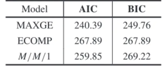
In Table 7 we show the values of the criterions AIC and BIC for the MAXGE distribution, ECOMP distribution andM/M/1. We observe that the MAXGE distribution has the lower values of AIC and BIC.
Table 7–Values of the criterions AIC and BIC.
Model AIC BIC
MAXGE 240.39 249.76
ECOMP 267.89 267.89
M/M/1 259.85 269.22
4.2 Real Data
Next, we analyze two real data: first of all, the express checkout of a Brazilian supermarket and secondly the accesses to the website.
4.2.1 The express checkout
A Brazilian supermarket was chosen to collect the data. It has ten normal checkouts and three express checkouts. In a particular day of collection of the data, one of the express checkouts had the same behavior of the studied system. The sample consists of the 85 service times in minutes.
In Table 8 we show the summary of the express checkout data. We observe that the maximum service time is 5.93 minutes and the minimum service time is 1.6 minutes.
Table 8–The summary of the express checkout data. Mean Median Maximum Minimum Standard-deviation
1.12 1.05 5.93 1.6 0.95
We use the Kolmogorov-Smirnov test to check whether a sample comes from a population with exponential distribution(H0). Therefore, with the significance levelα = 0.05 and p-value=
0.3497 the null hypothesis is not rejected for the exponential distribution (Lilliefors, 1967).
In Table 9 we show the MLEs of the parametersρ andλ, the confidence intervals (CI) 95% and sde.
Table 9–The MLEs, confidence intervals (CI) 95% and sde.
Parameters MLEs CI(95%) sde
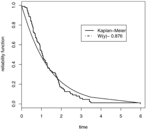
ρ 0.876 (0.86,0.89) 0.066
λ 0.91 (0.94,1.03) 0.044
Using the Equation (9) withr = 1 and we truncated the sum in the sample size. We obtain
E(Y)=2.72 minutes for the maximum service time.
In Figure 4 we compare the reliability function of the MAXGE distribution with the estimated reliability function. We observe that the reliability function of the MAXGE distribution fits with the estimated reliability function.
Figure 4– Comparison between the reliability function of the MAXGE distribution and the estimated reliability function.
In Figure 5 we compare the MAXGE distribution, ECOMP distribution andM/M/1 model.
In Table 10 we show that the MAXGE distribution has the lower values of the criterions AIC and BIC.
4.2.2 The accesses to the website
Figure 5–Comparison between the reliability functions of the MAXGE distribution, ECOMP distribution andM/M/1 model.
Table 10–Value of the criterions AIC and BIC.
Model AIC BIC
MAXGE 191.90 190.57 ECOMP 192.72 193.80
M/M/1 192.20 191.00
data are of the Midia group). For this purpose, a survey with 26 questions was allocated on this website. The survey was distributed through social networks (Facebook, Twitter, Orkut, MySpace, Youtube) and 1,000 emails were sent to the main communication agencies in Brazil. On the website “Tendˆencias Profissionais”, the arrivals and the outputs of the customers were registered. Data collection started on 20 October, 2010 and it was available for 20 days. We analyze in a particular day which we collected 385 accesses on website.
For access the Tendˆencias Profissionais:
(http://tendenciasprofissionais.wordpress.com/grupodepesquisa-mid/).
In Table 11 we show the summary of the accesses on website. We observe that the maximum time inter-access is 15.2 seconds and the minimum inter-access is 0.0001 seconds.
Table 11–The summary of the accesses on webite in seconds. Mean Median Maximum Minimum Standard-deviation
The Kolmogorov-Smirnov test was used to check whether a sample comes from a population which is exponential distributed(H0), with the significance levelα=0.05 andp-value=0.2497
the null hypothesis is not rejected for the exponential distribution.
On the website each access can be considered a service channel, therefore, the service rate de-pendent of the state of the system, in this case the pressure parameter assumes values one,φ. For this reason, a possible model for the maximum inter-access is the MAXPE distribution.
In Table 12 we show the MLEs of the parametersρandλ, the confidence intervals 95%(CI) and sde for the parameters.
Table 12–The MLEs, the confidence intervals 95% (CI) and the sde for the parameters of the MAXPE distribution.
Parameter MLEs CI(95%) sde
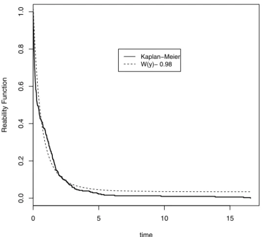
ρ 0.978 (0.916,1.039) 0.335
λ 0.901 (0.862,0.933) 0.094
We calculate theE(Y)by Equation (12) with r=1. We truncated the sum in the sample size and we obtainE(Y)=8.42 seconds.
In Figure 6 we compare the reliability function of the MAXPE distribution with the estimated reliability function. We observe that the reliability function of the MAXPE distribution is a closely concordance with estimated reliability function.
0 5 10 15
0.0
0.2
0.4
0.6
0.8
1.0
time
Reability Function
Kaplan−Meier W(y)− 0.98
In Figure 7 we compare the MAXPE distribution with theM/M/∞model.
Figure 7– Comparison between the reliability functions of the MAXPE distributionwith theM/M/∞
model.
In Table 13 we observe that the MAXPE distribution has the lower values criterions AIC and BIC, therefore, the MAXPE distribution is the best model.
Table 13–Value of the criterions AIC and BIC.
Distributions AIC BIC
MAXPE 140.640 148.112
M/M/∞ 213.81 212.030
5 CONCLUSIONS
increases proportionally of the state of the system, the new service channels are open and the MAXCOMPE distribution becomes the MAXPE distribution. Finally, forφ → ∞the service is very fast, we observe only one customer in the system and the MAXCOMPE distribution becomes the MAXBE distribution. The properties of the proposed distribution are discussed, including a formal proof of its density function and moments. To illustrate the applicability of the model the simulations and real date are used. We simulated two systems with different traffic intensities, such as,ρ =0.8 and 0.9. These values are chosen, because the studied system has heavy traffic, for this reason, the parameter of the traffic intensity has high values. A restriction is the used the small traffic intensity because the MAXCOMPE distribution is zero truncated, therefore, the system is never idle. Furthermore, we observed that the sample mean of the esti-mates of the parameters is near of the true value. In addition, the fit of the proposed model was better when compared with the models: ECOMP,M/M/1 andM/M/∞. We used the criterions AIC e BIC to select the best distribution to explain the data. We used two real data, data of the express checkout for illustrated the MAXGE distribution where there is single server. And data of the access on the website for illustrated the MAXPE distribution. To conclude, we believe that the MAXCOMPE distribution has a practical approach and it can be applied to various practical situations.
APPENDIX
In this appendix, we show the programs in software R used in this paper and the truncation of the sum inE(Y).
1. The programs in software R used in this paper.
• Programs in software R to simulate the M/M/1 model, Test Log-rank and Chi-squared tests.
require(VGAM)
rej log=0
rej chi =0
f or(ii n1 :1000)n =10000 stop
nat=1 number of the channels λ=0.9 the arrival rate
mi =1 the service rate v=vect or()
cust omers.arr ival =0
cust omes.service =0
cust omers.queue=0
s yst em =numeric(n)
time = numeric(n)
t ime−wait =numeric(n)
clock1=numeric(nat)
y=vect or()
t ime−service =numeric(n)
alarm−clock=rep(−1,nat)
f or(i;in2:n)
{
time.atual =(i−1)∗0.1 time[i] =(i−1)∗0.1 arrival =r pois(1, λ∗0.1)
customers-arrival= customers-arrival + arrival customers-queue = customers-queue + arrival system[i] = system[i-1] + arrival
if(sum(alar m−clock== −1) >0 andcust omers−queue>0)
{
vagas =sum(alarm−clock == −1) if(place! =sum(alarm−clock== −1))
}stop(”non con f orming suposit ions!”)
}minimum = min(place,customers-queue) for (j in 1:minimum){clock=rex p(1,0.9)
clock1[which(alar m−clock== −1)[1]] =clock
alarm−clock[which(alar m−clock== −1)[1]] =t ime.at ual+clock cust omers−queue=cust omers−queue−1}
}
f or(j in1:nat)
{if(t ime.at ual >=alarm−clock[j]e alarm−clock[j]! = −1){s yst em[i] = s yst em[i] −1
alarm−clock[j] = −1
cust omers−service=cust omers−service+1
y[cust omers−service] =clock1[j] clock1[j] =0}
}
Log-rank and Chi-squared testst ime=c(y,s2)
group=c(rep(0,lengt h(y)),r ep(1,lengt h(s2)))
st at us=rep(1,lengt h(y)+lengt h(s2))
s=survdi f f(Surv(t ime,st at us==1)group,dat a=mice)
schi =chisq.t est(y,s2) if(schisq >3.84)
{
rej log=rej log+1
}
if(schi p.value <0.05)
{
rej chi <−rej chi+1
} }
• Program reliability function and estimated reliability function by Kaplan-Meier method.
dado<−cbind(y,cens=1)
s2=numeric()
mu=0.9 traffic intensity
sigma=0.9 service rate
s2=ex p(mu∗(1−ex p(−sigma∗y)))∗ex p(−sigma∗y)/(ex p(mu)−1)MAXPE distribution
s2 =ex p(−y∗sigma)∗(1−mu)∗sigma/(1−mu∗(1−ex p(−y∗sigma))) MAXGE distribution
requir e(survival)
t empos=dado[,1] cens=dado[,2]
ekm =survf it(Surv(y,cens)1)
plot(ekm,lt y=1,lwd =2,con f.int =F,xlab=“t ime”,
ylab=“reliabili t y f unct ion”)
lines(y,s2,col =′ blue′,lt y=1,lwd =2)
t ext(7,1,“tra f f icint ensit y =0.8”)
legend(3,0.8,c(′M/M/1′,′W(y)=0.876′),bt y=′1′,lt y=c(1,4,3,2),
lwd =c(2,2,2,2))
• Program optim for the MLEs. verosi <−f unct ion(param){
mu<−param[1] sigma<−param[2]
i f(any(mu<1e−200))ret urn(.Machi nedouble.xmax.5)
f =sigma∗(ex p(−sigma∗y))∗(1−mu)/(1−mu∗(1−ex p(−sigma∗y)))2 MAXGE distribution
lv <−log(f)
sum(−lv)
}
est ima <−opt im(c(0.888,0.9), verosi,met hod =“B F G S”,hessian =T); est ima
est imahessian
solve(est imahessian)
• Criterions AIC and BIC
lm1<−lm(smax 1)
AI C(lm1)
st opi f not(all.equal(AI C(lm1),
AI C(log L ik(lm1))))
B I C(lm1)
lm2<−updat e(lm1, . .−E xaminat ion)
AI C(lm1,lm2)
B I C(lm1,lm2)
2. The truncation of the sum inE(Yr)for all the models:
TheE(Yr)is
E(Yr)= λ
−rŴ(r+1)ρ [Z(ρ , φ)−1]
∞
m=1 mρm−1
(m!)φ m−1
k=0
(−1)k m−1
k
1 (1+k)r+1.
We have an upper bound as
∞
m=1 mρm−1
(m!)φ m−1
k=0
(−1)k m−1
k
1 (1+k)r
τ
<
∞
m=1 mρ
m−1
(m!)φ.
The seriesτ has an upper bound given by the series ∞m=1m
ρm−1
(m!)φ that is convergent
(Minka et al., 2003) because
lim
m→∞m
ρm (m!)φ =0.
Furthermore, it is possible to truncate the seriesτ at someν-th term such that
ν
m=1 mρm−1
(m!)φ m−1
k=0
(−1)k m−1
k
1 (1+k)r+1
+
∞
m=ν+1 mρm−1
(m!)φ m−1
k=0
(−1)k m−1
k
1 (1+k)r+1,
where
Rν =
∞
m=ν+1 mρm−1
(m!)φ m−1
k=0
(−1)k m−1
k
1 (1+k)r+1.
whereRνis absolute truncated error.
An upper bound can be found based in the seriesρm/(m!)φ,m=1,2, . . . ,, decreases at a faster rate then a geometric series. Thus, there exists 0< εν <1 for allm > ν, so that
ρ/(m+1)φ< ε
νTherefore, Rν < εν, the error is small.
REFERENCES
[1] ADAMIDISK, DIMITRAKOPOULOUT & LOUKASS. 2005. On an extension of the exponential-geometric distribution.Statistics & probability letters,73(3): 259–269.
[2] AKAIKEH. 1974. A new look at the statistical model identification.Automatic Control, IEEE Trans-actions on,19(6): 716–723.
[3] BARRETO-SOUZAW,DEMORAISAL & CORDEIROGM. 2011. The weibull-geometric distribu-tion.Journal of Statistical Computation and Simulation,81(5): 645–657.
[4] BARTHW, MANITZM & RAIKS. 2010. Analysis of two-level support systems with time-dependent overflow a banking application.Production and Operations Management,19(6): 757–768.
[5] BEKKERR, BORSTS, BOXMAO & KELLAO. 2004. Queues with workload-dependent arrival and service rates.Queueing Systems,46(3): 537–556.
[6] BEKKERRGK, NIELSENB & BANGT. 2011. Queues with waiting time dependent service. Queue-ing Systems,68(1): 61–78.
[7] BOXMAO & VLASIOUM. 2007. On queues with service and interarrival times depending on waiting times.Queueing Systems,56(3): 121–132.
[8] CANCHOVG, LOUZADAF & BARRIGAGD. 2011. The geometric-birnbaum–saunders regression model with cure rate.Journal of Statistical Planning and Inference.
[9] CORDEIROGM, RODRIGUESJ &DECASTROM. 2012. The exponential com-poisson distribution.
Statistical Papers, pages 1–12.
[10] DROGUETTEL & MOSLEHA. 2007. Time to failure assessment of products at service conditions from accelerated lifetime tests with stress-dependent spread in life. Pesquisa Operacional,27(2): 209–233.
[12] IYERSK & MANJUNATHD. 2006. Queues with dependency between interarrival and service times using mixtures of bivariates.Stochastic models,22(1): 3–20.
[13] JONGBLOEDG & KOOLEG. 2001. Managing uncertainty in call centres using poisson mixtures.
Applied Stochastic Models in Business and Industry,17(4): 307–318.
[14] KAPLANEL & MEIERP. 1958. Nonparametric estimation from incomplete observations.Journal of the American statistical association,53(282): 457–481.
[15] KIMURAT. 1991. Approximating the mean waiting time in the gi/g/s queue.Journal of the Opera-tional Research Society, pages 959–970.
[16] KLEINBAUMDG & KLEINM. 2012. Kaplan-meier survival curves and the log-rank test. InSurvival analysis, pages 55–96. Springer.
[17] LILLIEFORSHW. 1967. On the kolmogorov-smirnov test for normality with mean and variance un-known.Journal of the American Statistical Association,62(318): 399–402.
[18] MARINCV, DRURYCG, BATTAR & LINL. 2007. Server adaptation in an airport security system queue.OR Insight,20(4): 22–31.
[19] MASSEYJRFJ. 1951. The kolmogorov-smirnov test for goodness of fit.Journal of the American statistical Association,46(253): 68–78.
[20] MINKATP, SHMUELIG, KADANEJB, BORLES & BOATWRIGHTP. 2003. Computing with the com-poisson distribution.Pittsburgh, PA: Department of Statistics, Carnegie Mellon University.
[21] MORABITOR &DELIMAFC. 2000. Um modelo para analisar o problema de filas em caixas de supermercados: um estudo de caso.Pesquisa Operacional,20(1): 59–71.
[22] RIGBYR & STASINOPOULOSD. 2005. Generalized additive models for location, scale and shape.
Journal of the Royal Statistical Society: Series C (Applied Statistics),54(3): 507–554.
[23] SCHWARZGET AL. 1978. Estimating the dimension of a model.The annals of statistics,6(2): 461– 464.
[24] SHARMAK & SHARMAG. 1994. A delay dependent queue without pre-emption with general lin-early increasing priority function.Journal of the Operational Research Society, pages 948–953.
[25] WHITTW. 1989. Planning queueing simulations.Management Science,35(11): 1341–1366.
[26] WHITTW. 1990. Queues with service times and interarrival times depending linearly and randomly upon waiting times.Queueing Systems,6(1): 335–351.