Repositório ISCTE-IUL
Deposited in Repositório ISCTE-IUL:
2019-02-01Deposited version:
Post-printPeer-review status of attached file:
Peer-reviewedCitation for published item:
Barraza, N., Moro, S., Ferreyra, M. & de la Peña, A. (2019). Mutual information and sensitivity analysis for feature selection in customer targeting: a comparative study. Journal of Information Science. 45 (1), 53-67
Further information on publisher's website:
10.1177/0165551518770967Publisher's copyright statement:
This is the peer reviewed version of the following article: Barraza, N., Moro, S., Ferreyra, M. & de la Peña, A. (2019). Mutual information and sensitivity analysis for feature selection in customer
targeting: a comparative study. Journal of Information Science. 45 (1), 53-67, which has been published in final form at https://dx.doi.org/10.1177/0165551518770967. This article may be used for non-commercial purposes in accordance with the Publisher's Terms and Conditions for self-archiving.
Use policy
Creative Commons CC BY 4.0
The full-text may be used and/or reproduced, and given to third parties in any format or medium, without prior permission or charge, for personal research or study, educational, or not-for-profit purposes provided that:
• a full bibliographic reference is made to the original source • a link is made to the metadata record in the Repository • the full-text is not changed in any way
Mutual information and sensitivity
analysis for feature selection in
customer targeting: a comparative
study
Abstract
Feature selection is a highly relevant task in any data-driven knowledge discovery project. The present research focus on analysing the advantages and disadvantages of using mutual information (MI) and data-based sensitivity analysis (DSA) for feature selection in classification problems, by applying both to a bank telemarketing case. A logistic regression model is built on the tuned set of features identified by each of the two techniques as the most influencing set of features on the success of a telemarketing contact, in a total of 13 features for MI and 9 for DSA. The latter performs better for lower values of false positives while the former is slightly better for a higher false positive ratio. Thus, MI becomes a better choice if the intention is reducing slightly the cost of contacts without risking losing a high number of successes. On the other side, DSA achieved good prediction results with less features.
Keywords
Feature selection; mutual information; sensitivity analysis; customer targeting; direct marketing; modelling.
1. Introduction
Customer targeting (CT) is a classical problem addressed by Business Intelligence (BI) methods and techniques. It involves finding the right target customers within the context of a marketing campaign for selling the campaign product or service [1]. Typical cutting edge approaches include using data mining (DM) for unveiling the potential knowledge through patterns of information hidden in big data repositories [2]. DM adopts the best practices inherited both from classical statistics and artificial intelligence, in an attempt to take advantage from both to enhance knowledge extraction from raw data [3].
In recent years, industries worldwide have experienced peaks and troughs of enthusiasm arisen from the high expectations of benefiting from novel technologies and approaches introduced by DM [4]. Discovering the best customers for targeting at a specific moment in time has proven to be NP-hard [5]. In real world, a vast number of characteristics and contextual specificities may potentially affect customer’s receptivity for acquiring a product. While recent technologies and DM procedures have progressively been increasing their capabilities of analysing large quantities of data, there is a growing need derived from data availability to identify which are the features that may potentially influence an outcome and which are those that are irrelevant and thus should be discarded, to avoid misleading DM algorithms [6]. As argued by [7] and [8], selecting the most meaningful features for understanding the underlying phenomena of interest often leads to a model obtained using a feature set significantly smaller and still valid in terms of performance when compared to the whole feature set for the studied problem. Also, the larger the number of features, the slower and more complex is the execution of the DM algorithm in pursuit for the best possible solution, given the exponential growth of possibilities that the algorithm needs to explore [9].
Hence, feature selection is a highly relevant task in any DM approach, constituting a key step where a large portion of the global effort should be spent on [10, 11].
Several techniques have been introduced and applied for feature selection. In [12] the authors conducted a survey, identifying three main methods, filter, wrapper, and embedded, while also mentioning the application of other techniques such as using unsupervised learning and ensemble methods. Table 1 summarizes their categorization.
Table 1. Feature selection methods.
Method Description Examples of techniques
Filter variable ranking techniques as the principle criteria for
variable selection by ordering Correlation criteria Mutual information Wrapper use the predictor as a black box and the predictor
performance as the objective function to evaluate the variable subset
Sequential selection algorithms Heuristic search algorithms Sensitivity analysis
Embedded reduce the computation time taken up for reclassifying different subsets which is done in wrapper methods by incorporating the feature selection as part of the training process
SVM-RFE (Recursive Feature Elimination)
Others several techniques that do not fit in the remaining three
methods Clustering Ensemble
Sensitivity analysis Adapted from [12].
Mutual information (MI) is one of the most widely adopted feature selection techniques, with the earliest studies dating back to the nineteen nineties [13]. The concept underlying MI is to measure the mutual dependence between two random features by identifying how much information of one of the features can be obtained from the other feature. Thus, it is linked to the entropy of a random feature, given by the amount of information held in the feature [14].
The usage of sensitivity analysis (SA) for feature selection in DM projects has been studied at least since the dawn of the new millennium [15]. The main idea behind SA is to assess model’s sensitivity to the variation of each of the input features on the predicted outcome: the more sensitive is the model, the more relevant is the effect of changing the input feature on the outcome. In this context, SA may be considered a wrapper method, according to the categorization identified in Table 1, even though SA may also be included within the model training process (thus, in this latter case, it would become an embedded method).
DM projects need to include a data preparation step, where usually occurs a feature selection procedure [16]. CT solutions initially consider a large set of features obtained from Customer Relationship Management (CRM) databases. Given CRM applications have been developed in course of time with new services to meet enterprises’ needs, it is crucial to find the smallest and most meaningful set of features that better characterises each customer to build effective marketing campaigns through accurate models. Being CT a typical problem addressed through DM, makes of it an ideal candidate for the application of feature selection methods. Thus, several studies were published related to the application of feature selection to CT [e.g., 17]. A recent study authored by [18] verses on the impact of feature selection in direct marketing. Their work analysed three filter methods for feature selection (correlation-based feature selection, subset consistency, and symmetrical uncertainty), concluding that symmetrical uncertainty resulted in better models, outperforming both the two remaining methods studied and a model without any feature selection procedure.
While there are several studies published on feature selection using MI, and a few using SA, none performed a direct comparison on both methods to assess the pros and cons on using each. Furthermore, even though a handful of recent studies were found comparing feature selection methods through practical applications [e.g., 18], none considered SA. The main contributions of this study are as follows:
• Comparing mutual information with sensitivity analysis for feature selection, by testing both methods on a real CT problem;
• Assessing the advantages and disadvantages of adopting each of the methods for feature selection, by cross-validating the results achieved on the experiments with the background literature on the subject;
• Drawing the insights on each method that may lead scholars and researchers on the adoption of each for a wide range of data-driven approaches to address real-world problems.
This paper is organized as follows. Next section presents a summary on the literature for MI, SA and feature selection applied to CT. In Section 3, the materials and methods adopted for the experiments are described. Results and
2. Background
This section outlines the theoretical background of the two analysed methods, mutual information and sensitivity analysis. Specifically, the application of both to feature selection is highlighted, as well as examples drawn from the literature are provided to better contextualize problems where each of the methods have been applied.
2.1. Mutual Information
Entropy and mutual information (MI) are well known concepts in Communications and Information Theory. They were originally introduced by Claude Shannon in a seminal paper [19], in order to find the optimal coding of a source on one hand and a noisy channel on the other. Entropy is related to the uncertainty or information content of a random variable. From this point of view, an event i having probability of occurrence pi has an information content of:
𝑖 = − log 𝑝𝑖 (1)
The base of logarithm defines the unit, base two logarithm gives units in bits. A more likely event implies that less information is disclosed when it occurs. The expectation of (1) computes the average information content of such set of events:
𝐻(𝑋) = − ∑ 𝑝𝑖log 𝑝𝑖 (2)
The expression (2) is the entropy of the random variable X in such a way that the event i corresponds to the value xi,
i.e., p(xi) = pi.
Entropy is bounded by the cardinality of the set of possible outcomes: H(X) ≤ log |X| and attains its maximum when the events follow a uniform distribution pi = 1 / |X|. The bigger the entropy, the more random are the events, thus, the
occurrence of an event gives more information, although it is less predictable. Considering two random variables with a given joint probability p(X, Y), the joint entropy is defined as:
𝐻(𝑋; 𝑌) = − ∑𝑥∈𝑋,𝑦∈𝑌𝑝(𝑥, 𝑦) log 𝑝(𝑥, 𝑦) (3)
And the conditional entropy is defined as:
𝐻(𝑋|𝑌) = − ∑𝑥∈𝑋,𝑦∈𝑌𝑝(𝑥, 𝑦) log 𝑝(𝑥|𝑦) (4)
MI between two random variables is defined as follows:
𝐼(𝑋; 𝑌) = − ∑ 𝑝(𝑥, 𝑦) log 𝑝(𝑥,𝑦)
𝑝(𝑥) 𝑝(𝑦)
𝑥∈𝑋,𝑦∈𝑌 (5)
From (5) the relation between MI and entropy may be derived:
𝐼(𝑋; 𝑌) = 𝐻(𝑋) − 𝐻(𝑋|𝑌) = 𝐻(𝑌) − 𝐻(𝑌|𝑋) (6)
MI definition can be extended to sets of random variables Xn = {X
1, X2, ..., Xn} and Yn = {Y1, Y2, ..., Yn}:
𝐼(𝑋𝑛; 𝑌𝑛) = − ∑ 𝑝(𝑥𝑛, 𝑦𝑛) log 𝑝(𝑥𝑛,𝑦𝑛) 𝑝(𝑥𝑛) 𝑝(𝑦𝑛)
𝑥𝑛∈𝑋𝑛,𝑦𝑛∈𝑌𝑛 (7)
where Xn and Yn are the set of outcomes of xn and ym.
A situation where redundant information can be removed arises when features are connected in a Markov chain: X1→
X2→Y. A well-known relation for this case is given by the data processing inequality I(X1;X2) ≥ I(X1;Y), an alternative
inequality is demonstrated in Lemma 1 in a similar way.
Lemma 1. If the random variables X1, X2, Y are connected in a Markov chain X1→ X2→Y, then:
(2) I(X2;Y) ≥ I(X1;Y)
Proof. Applying twice the chain rule to the MI:
𝐼(𝑋1, 𝑋2; 𝑌) = 𝐼(𝑋1; 𝑌|𝑋2) + 𝐼(𝑋2; 𝑌) = 𝐼(𝑋2; 𝑌|𝑋1) + 𝐼(𝑋1; 𝑌) (8)
By the Markov property:
𝐼(𝑋1; 𝑌|𝑋2) = 0 (9)
By replacing (9) in (8) and taking into account that the MI is always greater than 0 (e.g., reference [20]), from (8) and (9), it is computed that I(X2;Y) ≥ I(X1;Y), proving the lemma. It may be pointed out that both entropy and information
(e.g., H(X, Y) and I(X; Y)) functions from the information theory are quite suitable to eliminate redundant information, not generally taken into account with other methods.
A communication channel is a device or medium capable of transmitting information. The input information is carried out to the output. Since there is not a perfect mechanism for transmitting information, some noise is introduced in the communication process. Thus, the input and output information are not the same but related. MI may be used as a measure of that relation.
According to the source coding theorem, entropy is a measure of the average bits of information necessary to code the outcomes of a given random variable. Hence, H(X) is a measure of the input information to the channel, H(Y) is the information content at the output, I(X;Y) is the transmitted information, and taking into account the relations (6), H(Y|X) is a measure of the noise introduced by the channel. The conditional entropy H(X|Y) is called equivocation or ambiguity and it must be subtracted to the input information in order to obtain the transmitted information. According to the channel coding theorem, the MI gives the channel capacity and determines the maximum rate of information transmitted by the channel [20].
MI based feature selection consists in choosing the set of features raising most of the information of the output variable following a given criterion. The process starts by adding features from those carrying most of the information until a stopping criterion is reached. Since MI between the output variable Y and a given subset of input variables Xn is
given by:
𝐼(𝑋𝑛; 𝑌) = 𝐻(𝑌) − 𝐻(𝑌|𝑋𝑛) (10)
The estimation of I(Xn;Y) involves the estimation of the probability of the output Y given the set of features Xn, i.e.,
P(Y|Xn), implying that a larger set of features makes the estimation of P(Y|Xn) less reliable. Therefore, the maximum of
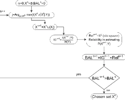
the product of information gain with reliability of estimation is used as the stopping rule, as indicated in the flowchart shown in Figure 1, which exhibits the MI feature selection approach. Other stopping rules for feature addition were considered in [21]. Note that the relative information gain 𝐼𝐺𝑛+1= 𝐼(𝑋𝑛+1; 𝑌)/𝐻(𝑌) goes from 0 when Xm and Y are
independent and H(Y|Xm) = H(Y) to 100% when Y is a deterministic function of Xm and H(Y|Xm) = 0. BAL stands for
balance (the supra index indicates the current step), a real number computed from the product of real numbers IG (Information Gain) and REL (chi square estimate confidence level). BAL is a compromise of gaining information and loosing accuracy (thus, the product IG x Rel) by adding a new feature. The algorithm stops when balance could not be incremented by adding any of the remaining features, and Xn results the selected features.
As a result, MI theory may help to cope with the task of feature selection by identifying the subset of features that minimizes H(Y|X), i.e., that maximizes the information underlying in the dataset, I(X;Y). Thus, features introducing further entropy in the communication channel may be discarded, helping to guide DM algorithms in building a model that understands the intrinsic relationships underneath the original data.
Figure 1. MI feature selection method.
2.2. Sensitivity Analysis
The usage of sensitivity analysis (SA) for providing insights on complex models dates back from the nineteen nineties, with a special emphasis on climate and environmental models [22, 23]. The advent of DM has introduced highly complex models with intrinsic convoluted relations that are hardly disentangled. Some of the most widely used of those models include machine learning algorithms such as neural networks in various formats and versions, and support vector machines.
SA has been proposed and analysed in the literature for input feature evaluation from data mining models. In Ref. [24] a computationally efficient one-dimensional method is presented, by varying one input at a time through its possible range of values and keeping the remaining input features constant. Subsequent studies explored further SA as a means for understanding the impact of the features that contributed to a model implementation had on the predicted outcome [15, 24]. By providing a procedure to evaluate the relevance of input features from models, several studies have included SA as a method for feature selection, hence choosing the most relevant features and discarding the least relevant [25]. Although SA requires that a model is previously available for assessing feature relevance since it focus solely on the features, it can virtually be applied to any type of predictive model.
Recent developments resulted in novel SA techniques such as the data-based SA (DSA), introduced by [26] in 2013. This procedure uses random samples from the data used to train the model for assessing feature relevance by changing the input features simultaneously, thus considering the relations between features (Figure 2). DSA has been applied since then in a large spectrum of domains and problems, such as bank marketing [27], wine quality assessment [28], jet grouting formulations [29] and social media performance metrics [30]. However, the only study using DSA specifically for feature selection is the work by Moro, Cortez and Rita, which applied such technique in a bank telemarketing case and resulted in a thread of published articles [6, 27, 17]. Their work adopted DSA but lacked in assessing the advantages and disadvantages of sensitivity analysis when compared to other feature selection methods. The present paper represents the first attempt in filling such gap.
Figure 2. Data-based sensitivity analysis.
2.3. Feature selection in customer targeting
CT is the marketing procedure of optimizing the selection of customers who to target within the context of a marketing campaign to meet campaign goals, usually, the acquisition of a product or service [31]. CT can be viewed as a branch of an integrated CRM strategy with a focus on building customer equity [32]. Other terms that are directly related to CT include direct marketing and database marketing, with the former being almost a synonymous [33], while the latter can be also associated with the need for a customer database to support CRM strategies [32]. CT provides an interesting ground for testing predictive machine learning techniques, with a large number of published studies alleging the discovery of predictive knowledge that may be used to benefit the success of CT [33]. Nevertheless, few of those works have seen a real production environment, effectively leveraging business [34].
Feature selection is a key task in every DM projects [10]. The main goal is to find the minimum set of features that optimize results translated in terms of model accuracy in fitting new data for the problem being addressed [2]. Also, by reducing the number of features used for modelling, the procedure for training the model becomes lesser computationally expensive, making it feasible to be executed on a daily or more frequent basis, for incorporating the subtle changes derived from immediate previous contacts [35]. For example, a bad news on the company or product widely spread through social media may directly affect the subsequent contacts [36]. Thus, model retraining for learning with new occurrences needs to occur often. One option is to use a rolling windows procedure where the window of data for training the model slides for keeping pace with time, an approach that may be adopted for several time evolving problems such as stock markets [37] and telemarketing [6]. The longer the algorithm takes to run the modelling procedure, the more likely the model does not adapt quickly enough to new information. Hence, selecting the right amount of features is in demand for problems with constant shifts in the influence features have on the outcome. Also, if information changes often, the feature selection procedure must be also frequently repeated, thus algorithm’s performance can become critical.
Feature selection using MI has been a subject of research in numerous problems. Moreover, studies are usually devoted to testing new feature selection approaches to well-known datasets, not focusing explicitly on the advantages to the business associated with the problems being addressed [38, 39]. However, no studies were found on feature selection using MI specifically focusing on CT, only a few papers published related to customer churning [40, 41]. DSA application to CT for feature selection has been the subject of study of [17], as stated in Section 2.2. The present study is focused in filling such void while at the same time performing a novel comparison between both methods, MI and DSA.
3. Bank telemarketing case study
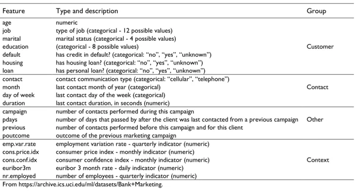
Bank telemarketing is a specific case of direct marketing where the customers of a bank are contacted and offered products or services through phone calls, although other direct channels such as email may be used [6]. For the experiments presented in this paper, the “Bank Marketing” dataset (file “bank-additional-full.csv”) published in the University of California Machine Learning Repository (http://archive.ics.uci.edu/ml/) was adopted. Such dataset was studied by numerous scholars and researchers, as the high number of page hits shows, above five hundred thousand. As a result, several studies have been published using its data, with the most for assessing machine learning and DM algorithms’ capabilities [41], and a few for feature selection [42]. This dataset encompasses a total of 41,188 phone contacts conducted by human agents from a Portuguese bank between 2008 and 2010, with the goal of selling an attractive long-term deposit, in an attempt of retaining customers’ financial assets in the institution. It should be stressed that all contacts are real, implying that it represents a real problem and to which feature selection may provide interesting benefits in reducing the features needed for modelling the outcome, choosing only influencing features while at the same time reducing model retraining duration. Each contact is characterized by twenty features, with some related to personal customer data (e.g., age), others to the contact itself (e.g., call duration) and previous calls made within the context of older campaigns (e.g., the outcome of previous contact), and the remaining related to the social and economic context that characterizes the country (e.g., number of employed people). Table 2 describes the list of features. More details can be obtained from [6]. The target outcome is the 21st feature from the dataset, concealing a binary value (yes/no) which represents the contact result: “yes” if the customer subscribed the deposit (total of 36,548 cases); “no” otherwise (total of 4,640 cases).
Table 2. List of input features.
Feature Type and description Group
age job marital education default housing loan numeric
type of job (categorical - 12 possible values) marital status (categorical - 4 possible values) (categorical - 8 possible values)
has credit in default? (categorical: “no”, “yes”, “unknown”) has housing loan? (categorical: “no”, “yes”, “unknown”) has personal loan? (categorical: “no”, “yes”, “unknown”)
Customer
contact month day of week duration
contact communication type (categorical: “cellular”, “telephone”) last contact month of year (categorical)
last contact day of the week (categorical) last contact duration, in seconds (numeric)
Contact campaign
pdays previous poutcome
number of contacts performed during this campaign
number of days that passed by after the client was last contacted from a previous campaign number of contacts performed before this campaign and for this client
outcome of the previous marketing campaign
Other emp.var.rate cons.price.idx cons.conf.idx euribor3m nr.employed
employment variation rate - quarterly indicator (numeric) consumer price index - monthly indicator (numeric) consumer confidence index - monthly indicator (numeric) euribor 3 month rate - daily indicator (numeric)
number of employees - quarterly indicator (numeric)
Context From https://archive.ics.uci.edu/ml/datasets/Bank+Marketing.
4. Experiments and results
4.1. Experimental setup
The bank telemarketing dataset was first assessed in terms of feature relevance by both methods studied, MI and DSA. Each method has its own specificities and procedures, as mentioned in sections 2.1 and 2.2. MI evaluates the amount of
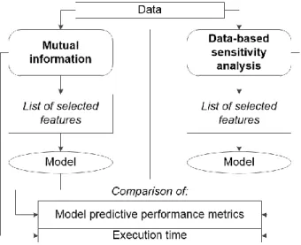
information concealed in each of the features, whereas DSA assesses the model in terms of the influence on the outcome by changing the input features. The experimental setup for the case of MI is solely the dataset with the data, as detailed in Section 2.1, while the DSA required that a model was previously built for assessing feature relevance in terms of the sensitivity of the model to changes on input features, as shown in Figure 2. Therefore, while MI selects the features according to the information each of them contains when compared to the remaining, DSA ranks features in terms of relevance for the model. For the latter, all the features that did not encompass individually at least 2% of relevance were discarded. Figure 3 summarizes the approach followed. The data initially used for both MI and DSA consisted in all features listed in Table 2 except for those that are only known after the call is made (“contact”, “month”, “day” and “duration”), which were removed.
Figure 3. Procedure undertaken.
In order to simulate a sliding window, the dataset was divided successively in different training and testing sets using a ten-fold cross-validation procedure. The test set is chosen by a window that takes 10% of the total records, starts at the first record and shifts to the next 10% of records without overlapping. In each experiment, the training set is composed by the other 90% records. At each fold, from the training set, the features were selected and used for building a predictive model which is applied to the testing set, in a procedure similar to [6]. At the end of the 10 fold experiments, a score of the probability of acquiring the offered product was computed for each contact. That score was then used to build the receiver operating characteristic curve (ROC) curve and find the confusion matrices shown below for different cut-off probabilities. The ROC plots the true positive rate (TPR), also known as sensitivity and recall, versus the false positive rate (FPR), which is the complement of the specificity, i.e., 1-specificity. Each point from the ROC curve represents a given threshold above which the target class is considered true. Thus, each point corresponds to a confusion matrix, which shows the predictive performance of the model by crossing the predicted value with the expected target. The selected features are then used for implementing a simple logistic regression (LR) model to fit data for predicting the outcome on the contacts. The usage of LR provides a direct means for measuring how modelling with the selected feature behaves in both cases, for allowing a direct comparison. While more complex machine learning techniques could be used (e.g., neural networks or support vector machines), the goal of the present study is to facilitate a comparison of both feature selection procedures, not putting emphasis on the modelling scenarios, where other studies have already focused on the analysed dataset. Also, to keep coherence in all experiments, the LR was also chosen for extracting feature relevance during feature selection from DSA. Additionally, since DSA is based on ranking feature relevance, for computing the model, all top ranked features with a summed relevance of at least 90% were included, discarding the remaining. Finally, the prediction results are analysed in the light of comparing both methods using both ROC and confusion matrices. Also, computational performance is evaluated, for a lighter method in terms of execution may allow a global frequently run learning procedure to be scheduled more often, as stated in Section 2.3.
4.2. Results
As remarked in [6], a predictive model does not hold any knowledge on future occurrences of the problem; thus, the dataset should be stripped off of any feature only known after contact execution, such as the call duration. Furthermore, in a real predictive system, a campaign is launched without knowing when the calls will be made, as these depend on both agent and especially client availability. Therefore, for the experimental setup, all features related to the current campaign were removed, namely: “contact”, “month”, “day” and “duration”. The only exception was “campaign”, which deserved a detailed analysis: this field indicates the number of contacts performed during this campaign, i.e., how many times was the contact rescheduled, which may happen due to several reasons, such as a machine answered the call and the agent decided to reschedule it, or the client asked to be recalled later. By taking into account that a telemarketing campaign can last a year, one may consider a dynamical model that take this field into account, incorporating multiple calls to the same client within the same campaign; therefore, this feature was included in the present analysis.
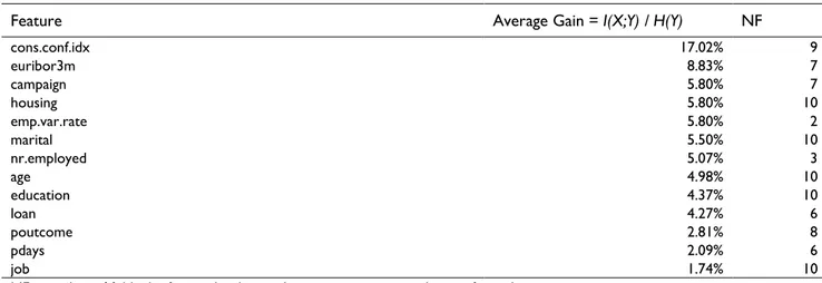
Since the software powerhouse1 performs segmentation process based on information theory, such product was chosen for obtaining the metrics. The software calculates the mutual information between each attribute and the output variable separately by estimating the joint probability, then, it chooses the set of variables carrying most of the information according to the criterion explained in sec. 2.1. Thus, in Table 3, the average gain shows the proportional mutual information between each feature and the output. The total information gain is then approximately 74.08%.
Table 3. Selected variables by the MI method.
Feature Average Gain = I(X;Y) / H(Y) NF
cons.conf.idx 17.02% 9 euribor3m 8.83% 7 campaign 5.80% 7 housing 5.80% 10 emp.var.rate 5.80% 2 marital 5.50% 10 nr.employed 5.07% 3 age 4.98% 10 education 4.37% 10 loan 4.27% 6 poutcome 2.81% 8 pdays 2.09% 6 job 1.74% 10
NF - number of folds the feature has been taken into account considering of its relevance.
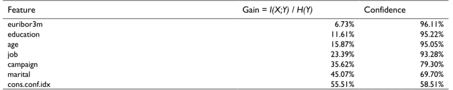
Elimination of redundant information occurs in the present data with the variable ”cons.price.idx”. This variable can be totally predicted by “cons.conf.idx” and “nr.employed” as shown in Table 4. As a result, we can say that the variables mentioned before are connected in a similar way as it was presented in lemma 1. Similar information content tables are shown for the other discarded features “default” (Table 5) and “previous” (Table 6). Confidence accounts for the accuracy in the estimation (Chi square), computed by summing up the squares of the differences between the expected and observed values. The sums of information gains for Tables 4, 5, and 6 are greater than 100%, since those account for non-independent features. Thus, redundant information is present, as the information raised by some features carries also information carried out by the other features.
Table 4. Information content and prediction of the variable “conf.price.idx”.
Feature Gain = I(X;Y) / H(Y) Confidence
cons.conf.idx 94.47% 96.11%
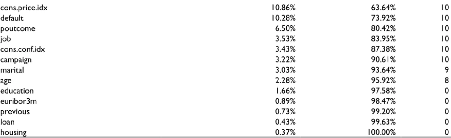
For the case of DSA feature selection, the R statistical tool was chosen2. R is an open source framework focusing on data analysis problems, allowing contributions with independent packages developed by numerous researchers worldwide [43]. Additionally, the “rminer” package implements the DSA algorithm [44]; therefore, it was adopted for all experiments related to DSA. Selected variables by DSA method are shown in table 7. As previously explained, it should be noted that within each fold of execution, all features summing up to 90% of global relevance were included. Interestingly, these features were considered for each of the ten folds, emphasizing its relevance for the problem and data being addressed.
Table 5. Information content and prediction of the variable “previous”.
Feature Gain = I(X;Y) / H(Y) Confidence
poutcome 83.11% 97.44%
nr.employed 86.02% 95.62%
pdays 87.59% 95.33%
job 89.42% 95.05%
education 91.94% 94.92%
Table 6. Information content and prediction of the variable “default”.
Feature Gain = I(X;Y) / H(Y) Confidence
euribor3m 6.73% 96.11% education 11.61% 95.22% age 15.87% 95.05% job 23.39% 93.28% campaign 35.62% 79.30% marital 45.07% 69.70% cons.conf.idx 55.51% 58.51%
A set of highly relevant features are selected based on the information content for MI, or based on model sensitivity to such features for DSA (Table 8). Considering the focus of this study is feature selection, a simple LR method was chosen for predicting contact outcome, for assessing the efficiency and accuracy of the features selected with both methods. This is the simplest algorithm of those analysed by [6]. The ROC curves for both models are drawn in Figure 4. It is possible to observe that LR with DSA feature selection (LR-DSA) outperformed MI (LR-MI). Since LR was also used to compute the model for applying DSA, an additional experiment was carried out using a support vector machine (SVM) to validate that such model (SVM-DSA) also outperformed LR-MI. Also, the LR ROC curve using all features is plotted on Figure 4 for comparison purposes. The decrease in performance is neglectable, thus supporting feature selection. It is interesting to highlight that LR-MI intersects with LR-DSA for an FPR of 0.5, with LR-DSA clearly achieving better performance for lower values of FPR, while LR-MI is slightly better above that value.
Table 7. Selected variables by the DSA method.
Feature Relative relevance (average) Summed relevance NF
emp.var.rate 26.29% 26.81% 10
cons.price.idx 10.86% 63.64% 10 default 10.28% 73.92% 10 poutcome 6.50% 80.42% 10 job 3.53% 83.95% 10 cons.conf.idx 3.43% 87.38% 10 campaign 3.22% 90.61% 10 marital 3.03% 93.64% 9 age 2.28% 95.92% 8 education 1.66% 97.58% 0 euribor3m 0.89% 98.47% 0 previous 0.73% 99.20% 0 loan 0.43% 99.63% 0 housing 0.37% 100.00% 0
NF - number of folds the feature has been taken into account considering of its relevance.
For further understanding the effects of using each predictive model built on each set of features, four confusion matrices are computed for MI and DSA methods. Table 9 shows the results extracted considering a typical cut-off probability 0.5, i.e., in which the most likely outcome is considered a success if the model predicts it with 50% or more of probability, and a cut-off lowered to just 10%, to account for the fact that this particular bank intends to increase efficiency with a especial emphasis on avoiding loosing successful contacts, considering lost deposit subscriptions directly implicates on missing business opportunities for retaining important financial assets in a crisis period (thus, the cost of losing a successful contact is much higher than the gain of avoiding a needless unsuccessful contact) [6]. Table 10 shows performance metrics for each of the approaches for the two cut-off points, as well as for the standard LR model with all the features. Generally, while there is a trade-off between metrics when comparing the three methods (including using all features), the results corroborate the findings from Figure 4, with LR-DSA achieving a performance just slightly below the LR model using all features.
Table 8. Selected features for both methods.
Feature MI DSA emp.var.rate X X pdays X X nr.employed X X cons.price.idx X default X poutcome X X job X X cons.conf.idx X X campaign X X marital X age X education X euribor3m X previous loan X housing X
Figure 4. ROC curves.
Table 9. Confusion matrices.
Cut-off probability MI method DSA method
Predicted Predicted
failure success failure success
Target Target 50% failure 36102 445 failure 36110 438 success 4391 250 success 3746 894 Target Target 10% failure 28583 7964 failure 27969 8579 success 1817 2824 success 1431 3209
Table 10. Performance metrics.
Cut-off probability Metric All features MI DSA
50% Cohen kappa 29.19% 6.63% 26.23% Accuracy 89.94% 88.26% 89.84% Sensitivity 98.53% 5.39% 19.27% Specificity 77.78% 98.78% 98.80% 10% Cohen kappa 28.26% 24.75% 27.32% Accuracy 76.81% 76.25% 75.70% Sensitivity 77.96% 60.85% 69.16% Specificity 32.27% 78.21% 76.53%
It is interesting to observe from the confusion matrices that an increasing number of false positives (FP) turn MI slightly better in predicting contact outcome than DSA, whereas DSA is clearly better for smaller FPs. Nevertheless, as stated previously, the results of MI maybe preferable if accounted that the cost of making a call is far less than the benefits of hitting a customer willing of getting the product. Another advantage of MI method is processing time, as
experiments conducted, MI procedure took just a few seconds, whereas DSA took around half a minute in an Intel{TM} I3 processor. This is a highly relevant benefit if more complex model techniques are used, as DSA depends on a model being built first. Furthermore, such advantage may be particularly emphasized for larger datasets.
4.3. Discussion
Comparing tables 7 and 3 several important remarks may be stated:
• Both feature selection methods clearly achieve different results.
• The most relevant features for one method is considered as little relevant for the other. Such is the case of “emp.var.rate” and “cons.conf.idx”.
• Contrarily to MI, the number of features selected by DSA remains the same along the 10-fold experiments. • The set of features selected by MI is bigger than that selected by DSA.
The previous remarks lead to an interesting analysis. It seems to be that a given estimate like DSA does not reveal the inherent dependency among strongly correlated features. This situation can occur if the evaluation estimate considers a value where the independent variable does not lead to big variations in the estimate, like in a possible flat portion in the regression curve. This may be observed from Tables 7 and 3, where the features selected by DSA remain the same through the folds, contrarily to the MI method. Also, from the MI method, a feature can be discarded if there is not enough values as to get a good level of confidence, explaining why many variables were discarded in some folds, as shown in Table 3, column NF, for “emp.var.rate” and “nr.employed”.
It is possible to observe that MI has not taken into account the features “conf.price.idx”, “default” and “previous”; such finding has risen the interest in analysing how each of these variables are related to the remaining selected by MI. This analysis can be made from Tables 4, 5 and 6. Table 4 shows that “conf.price.idx” can be totally predicted by “cons.conf.idx” and “nr.employed”. Both of the latter features raise each one a given information of “conf.price.idx”. Thus, by combining them it is possible to predict “conf.price.idx” with an almost 100% of confidence. A similar case occurs with “previous”, as this feature can also be almost totally predicted by other selected variables, as it is shown on Table 5. Also, Table 6 exhibits that most of the information carried out by default is carried by other of the selected variables, thus it can be discarded.
Another interesting result comes out from the confusion matrices shown in Table 9. Similar behaviour results for the two cut-off probability of success, it can be seen that the MI method gives confusion matrices with very good specificity and bad sensitivity. Thus, the model hits many customers willing to get the product while at the same time failing by contacting many clients that would reject the offer. Hence, for the empirical experiments conducted, DSA may be qualified as more conservative, while the MI method is preferred when the cost of making a call is low and the income of selling the product is high. The ROC curves are similar, although the one obtained from the MI method is slightly worse given its greater number of false positives, as shown in Figure 4.
5. Conclusions
In this study, a comparison was conducted between two renowned feature selection methods, mutual information (MI) and the data-based sensitivity analysis (DSA). Advantages and disadvantages of both methods were shown. This important information can be used to decide the best method to use in a particular application. For the empirical procedure, a dataset containing more than forty thousand instances of the case of bank telemarketing was chosen. In this experiment, the advantages of applying the information theory concepts in order to eliminate redundant features were translated in a small subset of highly relevant features which enabled modelling faster and more accurately the outcome of clients subscribing or not a deposit. Also, the method allows getting the information content easily and rapidly, which allows that to be applied to big data sets. Since variables carrying most of the information of the output variable are selected by the proposed method, results have shown that a simple prediction algorithm such as logistic regression can be performed with good modelling results. On the other side, the data-based sensitivity analysis has the disadvantage of requiring a model for extracting feature relevance. Such drawback can halt a data mining project if the initial dataset holds a high number of features. Nevertheless, DSA does not require to dive deeply into the model for understanding which features are lesser relevant, for it is based on assessing outcome variation by also changing input features through their range of possible values. Using the tuned set of features obtained from each methods, in a total of 13 features for MI and 9 features for DSA from the initial 20, it is possible to observe from a logistic regression model built on each of
these two sets that the receiver operating characteristic curve from DSA outperforms MI model in the lower values of false positives, while MI is slightly better for a higher false positive ratio. Thus, if the goal of marketing managers is to reduce the number of calls made at the cost of eventually losing some successful contacts (true positives), then DSA feature selection resulted better for this case; otherwise, MI’s feature selection took a small lead. Such conclusion is highlighted in the confusion matrices obtained, with MI’s model achieving better results for predicting successes, while DSA outperforms MI on predicting failed contacts, i.e., when the client refused the deposit offered. For this specific case, losing a successful contact implicates eventual loss of the client’s financial asset, thus it is preferable to achieve a higher accuracy on predicting successes at the expense of wasting additional calls on unfruitful contacts. Nevertheless, the results are conclusive in that MI, although a rather old method, still achieves results comparable to other more recent methods, such as DSA.
Notes
1. http://www.dataxplore.com.ar/tecnologia.php#Powerhouse 2. https://cran.r-project.org/
Funding
<to be disclosed after blind peer review – Thank You>
References
[1] Turban E, Sharda R and Delen D. Decision Support and Business Intelligence Systems. 9th ed. USA: Pearson, 2011.
[2] Witten I, Frank E and Hall M. Data Mining: Practical machine learning tools and techniques. 3rd ed. USA: Morgan Kaufmann, 2011.
[3] Chen SY and Liu X. The contribution of data mining to information science. Journal of Information Science 2004; 30(6):550– 558.
[4] Gandomi A and Haider M. Beyond the hype: Big data concepts, methods, and analytics. International Journal of Information Management 2015; 35(2):137–144.
[5] Nobibon FT, Leus R and Spieksma FC. Optimization models for targeted offers in direct marketing: Exact and heuristic algorithms. European Journal of Operational Research 2011; 210(3):670–683.
[6] Moro S, Cortez P and Rita P. A data-driven approach to predict the success of bank telemarketing. Decision Support Systems 2014; 62:22–31.
[7] Liu H, Sun J, Liu L and Zhang H. Feature selection with dynamic mutual information. Pattern Recognition 2009; 42(7):1330– 1339.
[8] Guyon I and Elisseeff A. An introduction to variable and feature selection. Journal of Machine Learning Research 2003; 3:1157–1182.
[9] Wu X, Zhu X, Wu G-Q and Ding W. Data mining with big data. IEEE Transactions on Knowledge and Data Engineering 2014; 26(1):97–107.
[10] Domingos P. A few useful things to know about machine learning. Communications of the ACM 2012; 55(10):78–87. [11] Herzallah W, Faris H and Adwan O. Feature engineering for detecting spammers on Twitter: Modelling and analysis. Journal
of Information Science. Epub ahead of print 1 January 2017. DOI: 10.1177/0165551516684296.
[12] Chandrashekar G and Sahin F. A survey on feature selection methods. Computers & Electrical Engineering 2014; 40(1):16–28. [13] Battiti R. Using mutual information for selecting features in supervised neural net learning. IEEE Transactions on Neural
Networks, 1994; 5(4):537–550.
[14] Paninski L. Estimation of entropy and mutual information. Neural Computation, 2003; 15(6):1191–1253.
[15] Embrechts MJ, Arciniegas FA, Ozdemir M and Kewley RH. Data mining for molecules with 2-d neural network sensitivity analysis. International Journal of Smart Engineering System Design 2003; 5(4):225–239.
[16] Han J, Kamber M and Pei J. Data Mining: Concepts and Techniques. 3rd ed. USA: Morgan Kaufmann Publishers Inc., 2011. [17] Moro S, Cortez P and Rita P. A framework for increasing the value of predictive data-driven models by enriching problem
domain characterization with novel features. Neural Computing and Applications 2016; In press.
[18] Tan D-W, Yeoh W, Boo YL and Liew S-Y. The impact of feature selection: A data-mining application in direct marketing. Intelligent Systems in Accounting, Finance and Management 2013; 20(1):23–38.
[19] Shannon C. A mathematical theory of communication. Bell System Technical Journal 1948; 27:379–423.
[20] Cover TM and Thomas JA. Elements of Information Theory (Wiley Series in Telecommunications and Signal Processing). 2nd ed. USA:Wiley-Interscience, 2006.
[22] Homma T and Saltelli A. Importance measures in global sensitivity analysis of nonlinear models. Reliability Engineering & System Safety 1996; 52(1):1–17.
[23] Kewley RH, Embrechts MJ and Breneman C. Data strip mining for the virtual design of pharmaceuticals with neural networks. IEEE Transactions on Neural Networks 2000; 11(3):668–679.
[24] Kondapaneni I, Kordik P and Slavik P. Visualization techniques utilizing the sensitivity analysis of models. In: 39th conference on Winter simulation: 40 years! The best is yet to come (ed. J Tew), Washington, DC, USA, 9-12 December 2007, pp.730–737. IEEE Press.
[25] Liu Q, Zhao Z, Li Y-X and Li Y. Feature selection based on sensitivity analysis of fuzzy isodata. Neurocomputing 2012; 85:29–37.
[26] Cortez P and Embrechts MJ. Using sensitivity analysis and visualization techniques to open black box data mining models. Information Sciences 2013; 225:1–17.
[27] Moro S, Cortez P and Rita P. Using customer lifetime value and neural networks to improve the prediction of bank deposit subscription in telemarketing campaigns. Neural Computing and Applications 2015; 26(1):131–139.
[28] Cortez P, Cerdeira A, Almeida F, Matos T and Reis J. Modeling wine preferences by data mining from physicochemical properties. Decision Support Systems 2009; 47(4):547–553.
[29] Tinoco J, Correia AG and Cortez P. A novel approach to predicting Young's modulus of jet grouting laboratory formulations over time using data mining techniques. Engineering Geology 2014; 169:50–60.
[30] Moro S, Rita P and Vala B. Predicting social media performance metrics and evaluation of the impact on brand building: A data mining approach. Journal of Business Research 2016; 69(9):3341–3351.
[31] Cole AM. Internet advertising after sorrell v. ims health: A discussion on data privacy & the first amendment. Cardozo Arts & Entertainment Law Journal 2012; 30:283–315.
[32] Richards KA and Jones E. Customer relationship management: Finding value drivers. Industrial Marketing Management 2008; 37(2):120–130.
[33] Kim Y and Street WN. An intelligent system for customer targeting: a data mining approach. Decision Support Systems 2004; 37(2):215–228.
[34] Pinheiro CAR and McNeill F. Heuristics in Analytics: A Practical Perspective of what Influences Our Analytical World. USA: John Wiley & Sons, 2014.
[35] Liu H and Yu L. Toward integrating feature selection algorithms for classification and clustering. IEEE Transactions on Knowledge and Data Engineering 2005; 17(4):491–502.
[36] Goldenberg J, Libai B, Moldovan S and Muller E. The npv of bad news. International Journal of Research in Marketing 2007; 24(3):186–200.
[37] Romero-Meza R, Bonilla C, Benedetti H and Serletis A. Nonlinearities and financial contagion in latin american stock markets. Economic Modelling 2015; 51:653–656.
[38] Hoque N, Bhattacharyya D and Kalita JK. Mifsnd: a mutual information-based feature selection method. Expert Systems with Applications 2014; 41(14):6371–6385.
[39] Karimi S and Shakery A. A language-model-based approach for subjectivity detection. Journal of Information Science. Epub ahead of print 1 April 2016. DOI: 10.1177/0165551516641818.
[40] Idris A and Khan A (2012). Customer churn prediction for telecommunication: Employing various various features selection techniques and tree based ensemble classifiers. In: 15th International Multitopic Conference (INMIC), Islamabad, Pakistan, 13-15 December 2012, pp.23–27. IEEE Press.
[41] Verbraken T, Verbeke W and Baesens B. Profit optimizing customer churn prediction with bayesian network classifiers. Intelligent Data Analysis 2014, 18(1):3–24.
[42] Vajiramedhin C and Suebsing A. Feature selection with data balancing for prediction of bank telemarketing. Applied Mathematical Sciences 2014, 8(114):5667–5672.
[43] Ihaka R and Gentleman R. R: a language for data analysis and graphics. Journal of Computational and Graphical Statistics 1996; 5(3):299–314.
[44] Cortez P. Data mining with neural networks and support vector machines using the r/rminer tool. In: Advances in Data Mining. Applications and Theoretical Aspects. ICDM 2010. Lecture Notes in Computer Science, (ed. P Perner), Berlin, Germany, 12-14 July 2010, vol. 6171, pp.572–583. Springer.