Predictive analysis of incidents based on software deployments

(1)

Department of Information Science and Technology

Predictive Analysis of Incidents based on Software Deployments

José Diogo dos Santos Messejana

Dissertation submitted as partial fulfilment of requirements for the degree of Master in Computer Engineering

Supervisor:

Prof. Dr. Ruben Filipe de Sousa Pereira, Assistant Professor, ISCTE-IUL

Co-supervisor:

Prof. Dr. João Carlos Amaro Ferreira, Assistant Professor, ISCTE-IUL

(2)

(3)

i

Acknowledgements

First, I would like to thank the company that I worked with, that gave me all the necessary data to do this investigation, as well as all the people from the company that were available to clarify any doubts I had about the data that was given.

Second, I would like to thank everyone who helped and bared with me throughout this journey, who encouraged and did not let me give up on this when I had second thoughts. All the way from my friends who I had to skip out on sometimes, my co-workers at the company I work with, that always incentivised me to continue, both my supervisors who offered me the tools as well as for always being available to support me.

Finally, I would like to specially thank two group of people. First, my girlfriend, for always being there and never let me quit and giving me strength to continue and helping me out when I needed. Second, but most important my parents, because without them I would never be here writing this, they made every effort to give the tools, so that I could create my opportunities and ensured that I would never quit something after I started it.

(4)

Predictive Analysis of Incidents based on Software Deployments

(5)

iii

Resumo

Um número elevado de organizações de tecnologias de informação têm um grande número de problemas no momento e após lançarem os seus serviços, se juntarmos a isto o número elevado de serviços que estas organizações prestam diariamente, dificulta bastante o processo de Incident Management (IM). Um sistema de IM eficaz deve permitir aos decisores de negócio detetar facilmente estes problemas, caso contrário, as organizações podem ter de enfrentar imprevistos nos seus serviços (custos ou falhas). Esta tese irá demonstrar que é possível introduzir um processo de previsão que poderá levar a um melhoramento do tempo de resposta aos incidentes, assim como uma redução dos mesmo. Prevendo estes problemas estes podem alocar melhor os recursos assim como mitigar os incidentes. Como tal, esta tese irá analisar como prever esses incidentes, analisando os deployments feitos nos últimos anos e relacionando-os usando algoritmos de machine learning para prever os incidentes.

Os resultados mostraram que é possível prever com confiança se um determinado deploymente vai ou não ter incidentes.

(6)

(7)

v

Abstract

A high number of information technology organizations have several problems during and after deploying their services, this alongside with the high number of services that they provide daily, it makes Incident Management (IM) process quite demanding. An effective IM system needs to enable decision-makers to detect problems easily. Otherwise, the organizations can face unscheduled system downtime and/or unplanned costs. This study demonstrates that is possible to introduce a predictive process that may lead to an improvement of the response time to incidents and to the reduction of the number of incidents created by deployments. By predicting these problems, the decision-makers can better allocate resources and mitigate costs. Therefore, this research aims to investigate if machine learning algorithms can help to predict the number of incidents of a certain deployment.

The results showed with some security, that it is possible to predict, if a certain deployment will have or not an incident in the future.

(8)

(9)

vii

Publications

The author made a paper that was accepted in the 2019 International Conference of Data Mining and Knowledge Engineering from the World Congress of Engineering 2019 (Rank B).

(10)

(11)

ix

Index

Acknowledgements ... i Resumo ... iii Abstract ... v Publications ... vii Index ... ix Table index ... xi

Equation index ... xiii

Figure index ... xv

Abbreviations ... xvii

Chapter 1 – Introduction ... 1

Chapter 2 – Literature Review ... 3

2.1. Theoretical Background ... 4

2.1.1. Predictive Analysis ... 4

2.1.1.1 ML Algorithms types ... 5

2.1.1.2 Training and Evaluation ... 5

2.1.2. Incident Management ... 8

2.1.3. Software Deployment ... 9

2.2. Related Work ... 10

Chapter 3 – Work Methodology ... 15

3.1. Business and Data Understanding ... 17

3.2. Data Preparation ... 18

3.2.1 Initial Attribute Cleaning ... 18

3.2.2 Irrelevant Attributes ... 20

3.2.3 Irrelevant and duplicated entries ... 20

3.2.4 Efficiency Cleaning ... 20

3.2.5 Attribute Creation ... 20

3.2.6 Data Transformation ... 21

3.3. Modeling ... 22

3.4. Evaluation and Results ... 23

3.5. Deployment ... 28 Chapter 4 – Discussion ... 31 Chapter 5 – Conclusions ... 33 5.1. Research Limitation ... 33 5.2. Future Work ... 34 Bibliography ... 35

(12)

(13)

xi

Table index

Table 1 - Research Question ... 2

Table 2 - Selected Papers... 3

Table 3 - Related Work ... 11

Table 4 - Deployment Analysis ... 18

Table 5 - Incident Analysis ... 18

Table 6 - Number of Incidents Distribution ... 23

Table 7 - Naive Bayes results. Original (O), Weekends and Holidays (WH), Impact (IMP) ... 24

Table 8 - SVM results. Original (O), Weekends and Holidays (WH), Impact (IMP) .... 25

Table 9 - RF results. Original (O), Weekends and Holidays (WH), Impact (IMP) ... 26

Table 10 - CART results. Original (O), Weekends and Holidays (WH), Impact (IMP) 27 Table 11 - Algorithms best accuracy results comparison ... 28

(14)

(15)

xiii

Equation index

Equation 1 - Accuracy equation I ... 7

Equation 2 - Accuracy equation II ... 7

Equation 3 - Precision equation ... 7

Equation 4 - Recall equation ... 7

(16)

(17)

xv

Figure index

Figure 1 - Supervised Learning Algorithms (Myatt & Johnson, 2009)... 5

Figure 2 - CRISP-MD Levels (Wirth & Hipp, 2000) ... 15

Figure 3 - CRISP-MD model phases (Wirth & Hipp, 2000) ... 15

Figure 4 - CRISP-MD lifecycle overview Wirth & Hipp, (2000) ... 17

Figure 5 - Data prepartion workflow ... 19

Figure 6 - Final set of deployment attributes ... 21

Figure 7 - Final set of Incident attributes ... 22

(18)

(19)

xvii

Abbreviations

CART - Classification and Regression Trees

CRISP-DM - Cross Industry Standard Process for Data Mining DT - Decision Trees

IM - Incident Management IT - Information Technology

ITIL - Information Technology Infrastructure Library ITSM - Information Technology Management Process KNN - K-Nearest Neighbours

MDA - Multivariate Discriminant Analysis

ML - Machine Learning

NN - Neural Networks

RF - Random Forest

(20)

(21)

1

Chapter 1 – Introduction

Thousands of Information Technology (IT) organizations worldwide are struggling with the deployment of information technology service management processes (ITSM) and with the deployment of services into the daily IT operations(Jäntti & Järvinen, 2011). The number of IT services keeps increasing in countless different types of organizations where IT plays a leading role (Gacenga, Cater-Steel, Tan, & Toleman, 2011). Therefore, IT service managers are increasingly under pressure to reduce costs and quickly deliver cost-effective services (Aguiar, Pereira, Vasconcelos, & Bianchi, 2018) and consequently make Incident Management (IM) one of the most demanding ITSM processes.

Nowadays, many tickets are created each day (Mello & Lopes, 2015), especially in large-scale enterprise systems (Kikuchi, 2015; Lin et al., 2014). A recent study from Lou et al. (2017), and recently supported by Silva, Pereira, & Ribeiro (2018b), reported that about 12 billion lines of log messages are generated in their infrastructure each day for IM.

Most of the tickets are created with non-structured text (Lin et al., 2014) meaning that they can have numerous variations on the description of it and organizations are not able to extract value from such data.

An effective IM system needs to enable decision-makers to detect anomalies and extract helpful knowledge to solve incidents(Aguiar, Pereira, Vasconcelos, & Bianchi, 2018). These incidents can lead to unscheduled system downtime and/or unplanned costs (Russo, Succi, & Pedrycz, 2015) and cause a significant impact since the recovery process can require time and resources that were not considered (Fulp, Fink, & Haack, 2008). Furthermore, if system administrators are able to predict these incidents, they can better allocate their resources and services to mitigate the costs (Russo et al., 2015). Predicting computer failures can help in mitigating the impact even when the failure is impossible to solve because recovery and rescue can be taken way earlier (Fronza, Sillitti, Succi, & Vlasenko, 2011) and allow managers to get a better response over system performance (Russo et al., 2015).

Predictive Analysis can help in to predict future incidents by using retrospective and current data (Kang, Zaslavsky, Krishnaswamy, & Bartolini, 2010). In recent years, machine learning (ML), as an evolving subfield of computer science has been widely used in the challenging problem of predicting incidents as well as anomaly detection problems

(22)

Chapter 1 – Introduction

2

(Tziroglou et al., 2018) providing information on the applications and the environments where the applications are deployed (Oliveira, 2017).

As previously stated, organizations produce and report billions of incidents each day, making it difficult for organizations to keep up with it. Predictive analysis can be used to predict some of those incidents and therefore reduce their occurrence and the possible costs associated with them.

Software deployments can have critical information to predict and therefore prevent incidents, like a feature that often causes many incidents when there is a deployment with it. Therefore, this research aims to analyze if it is possible to predict incidents based on the software deployment information of the last few years to build a predictive model capable of predicting those incidents and in the end answer the research question in Table 1.

Table 1- Research Question

ID Description

RQ1 Can software deployments information be used to predict incidents?

This research uses the Cross-Industry Standard Process for Data Mining (CRISP-DM) as a research methodology. This methodology aims to create a precise process model for data mining projects (Chapman et al., 1999).

This research will start by exposing what already exists in the literature and how it relates to this research. Then the main concepts will be shortly explained as well as the methodology that will be followed. On chapter 3, it is exposed what was done on this research and on the following chapters, a discussion of the results obtained as well as the conclusions will be presented.

(23)

3

Chapter 2 – Literature Review

The Literature Review research was made between the 12th _{of August 2018 through} the 30th_{of December 2018.}

The acceptance criteria of the papers in Table 2 was done as follows. First based on the relation of the title with the three big topics, then if it had any relation, an analysis of the abstract would be done to see if it indeed would relate to this study and if so a quick analysis of the content was done to check if there was relevant content to be applied in this study. Only english written papers were selected. The numbers in Table 2 represent the papers that matched the criteria and endend being used in this document

The research was made as follows:

Table 2 – Selected Papers

Keywords

#Selected papers

Total Google

Scholar ACM Springer IEEE

P re dictive A na lysi s Predictive Analysis 3 4 1 0 8 Incident Predictive Analysis 0 3 2 0 5 Predictive Model 0 2 0 0 2

Support Vector Machines 0 1 0 0 1

Prediction on software

logs 0 0 3 0 3

Software logs 0 0 1 0 1

Predicting incidents 0 1 0 0 1

Predicting incident ticket 0 2 0 0 2

Prediction deployment 1 0 0 0 1 Inc ident Ma na ge ment Incident Management it 1 0 0 0 1

Incident Management itil 2 0 0 0 2

Incident Management 0 1 0 0 1 It Incident Management 0 1 1 2 4 S oftw are De ploym ent Software Deployment Quality 1 0 0 0 1 Software Deployment 1 2 0 0 3 Software Deployment Process 0 1 0 0 1 Software Deployment Incident 0 0 0 1 1 Total 9 18 6 3 36

(24)

Chapter 2 – Literature Review

4

As seen in Table 2, the search was made around the three main concepts that will be explained in the following sub-chapters.

At the end it was not found any studies relating predictive analysis and software deployment to predict incidents, so the scope was made wide again and started searching for predictive analysis related to logs which have some relation to software deployment messages. It was also searched for Support Vector Machines since it was one of the most used algorithms found in the literature. In IM, it was once again used a wide scope and then narrowed to only IT IM. ITIL was searched after reading it in the IM literature.

2.1.Theoretical Background

This research grounds on three main concepts: Predictive Analysis, Incident Management, and Software Deployment. The next paragraphs briefly detail each of these concepts.

Predictive analysis can be defined as the act of doing predictive analytics. Predictive Analytics is the combination of techniques that can help to make informed decisions by doing an analysis of historical data (Myatt & Johnson, 2009).

IM is said to be one of the most important ITIL process model elements for the delivery of IT services (Kang et al., 2010). The goal of IM is to bring normal service operation as fast as possible, after a service disruption (Bartolini, Stefanelli, & Tortonesi, 2010) and finding a resolution for the incident while minimizing business impact which has an important role in creating a highly scalable system.

Software deployment can be defined as being the group of processes between the acquisition and execution of software (Dearle, 2007; Mukhopadhyay, 2018) and the connection between software components and its hardware (Medvidovic & Malek, 2007).

2.1.1. Predictive Analysis

Predictive analysis allows estimations of the impact of design decisions, that can help to get optimal operational results (Oliveira, 2017). Existing methods in the literature can be classified broadly into two categories: lockset analysis and feasibility guarantee (Wang, Kundu, Limaye, Ganai, & Gupta, 2011). While lockset analysis methods strive to cover all the true positives, but may also introduce many false positives, feasibility guarantee methods ensure all the reported bugs can happen, but they may not cover all the detectable errors (Wang et al., 2011).

(25)

5

The following sub-sections will review the different topics related to predictive analysis and ML.

2.1.1.1 ML Algorithms types

There can be three types of ML algorithms:

• Supervised Learning – If the objective is to predict something based on known data (Bari, Chaouchi, & Jung, 2014);

• Unsupervised Learning – If the objective is to predict something, but there is no data available (Kotsiantis, 2007);

• Reinforcement Learning – Where the algorithm learns based on rewards and tries to maximize that reward (Bari et al., 2014).

Since this research will use a supervised learning algorithm, there will not be any focus on the other two.

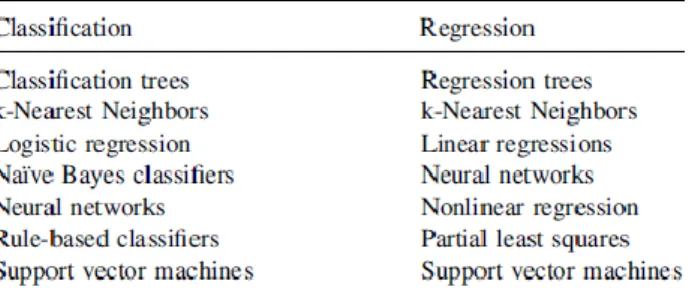
As for supervised learning, it can be split into two categories of tasks, which are classification and regression.

In classification the results are categorical variables meaning that it can only take a strict number of values (Myatt & Johnson, 2009), this category aims to predict the category of a field (Myatt, 2007) or if something will happen or not, for example, if there will or not be an incident for a deployment. On the other hand, in regression the results are continuous variables meaning that this category of the task is used to make estimations and predictions (Myatt & Johnson, 2009), for example, how many incidents will a deployment generate.

Figure 1 shows a list of supervised learning algorithms and their corresponding task category.

Figure 1 - Supervised Learning Algorithms (Myatt & Johnson, 2009)

2.1.1.2 Training and Evaluation

After the data is prepared, it is now necessary to train the model in order to better generalize the relation of the inputs and outputs, and then we need to evaluate the training. The quality of the model is based on its ability to accurately predict based on a certain

(26)

6

number of inputs. The model should neither overgeneralize or overfit the relation (Myatt, 2007). Starting by the training phase, this phase can be done in two different ways, either splitting the dataset in a train set and a test set or by using cross validation.

Splitting the dataset in a train and test set will allow the model to ignore the data that was used in the test set, and so, the model will only be built with a part of the dataset (train set) (Myatt, 2007), the model will then produce results that will be compared with the test set to evaluate the model (Brownlee, 2016). The percentage of the split is different depending on the dataset that is being used (Myatt, 2007), although the recommended values throughout the literature are between 70%-30% up to 80%-20% (train-test).

In cross-validation a model learns its weights and parameters on a training set and calculates its prediction performance on the new instances of a validation set (Bishop, 1996). The dataset is split in k smaller datasets (the most used values for k are 3, 5, and 10), but similar to the previous approach it depends on each dataset, as the k has to allow each dataset to be large enough (Brownlee, 2016). Each time one of the data set is used for testing the remaining ones are used together for training, this then iterates until every data set is used as a test set (Bari et al., 2014). After all the datasets are used as test sets, several score performances are given, which can then be interpreted by applying the mean and standard deviation. As the algorithm runs several times with different datasets, it ends being more reliable than the split approach (Brownlee, 2016).

Identification of the best performing classifiers can be made by feature reduction independently from data manipulation in cross-validation. Splitting the dataset is beneficial to classification problems since data splitting increments the diversity of the sets and the strength of the classification result (Russo et al., 2015).

After all the training, several metrics can be used to evaluate the results.

There are four possible outcomes of the prediction (Hovsepyan, Scandariato, & Joosen, 2016):

• True positive (TP) if it was predicted and was indeed an accurate prediction; • True negative (TN) if it was not predicted like it should not have been; • False-positive (FP) if it was predicted, but it should not have been; • False-negative (FN) if it was not predicted, but it should have been. These outcomes can then be used to create different metrics, such as:

(27)

7

• Accuracy – Most used metric in classification (Brownlee, 2016). Closer to 1 means a better result (Myatt & Johnson, 2009). Accuracy can be obtained, as shown in Equation 1 and Equation 2.

Equation 1- Accuracy equation I

Equation 2- Accuracy equation II

• Precision – Number of correct results divided by the number of guesses (Manning, Raghavan, & Schuetze, 2009). This is shown in Equation 3.

Equation 3- Precision equation

• Recall – Number of correct results guessed in all the possible correct results (Manning et al., 2009). This is shown in Equation 4.

Equation 4- Recall equation

• ROC curve – Only used in classification models (Brownlee, 2016). It relates the precision with recall (Myatt, 2007). If the curve grows quickly on the left side, it means that the model is good (Manning et al., 2009).

• F-measure – Relates precision with recall by doing a weighted harmonic mean between them (Manning et al., 2009). This is shown in Equation 5.

Equation 5- F-measure equation

Imbalanced data can be an issue when someone wants to evaluate the performance of posterior probabilities. According to Hongyu Zhang & Xiuzhen Zhang (2007), the measures introduced in Menzies, Greenwald, & Frank (2007), true and false positive rate are not enough in case of imbalanced data. When data is imbalanced, Hongyu Zhang & Xiuzhen Zhang (2007) prove that models can be able to detect faults (true positive rate is

(28)

8

high) and raise few false alarms (false positive rate is small) but still be very poor in performance (precision is small). Precision is an unstable measure and should not be used alone. Classification results with low precision and high true positive rate are useful and very frequent in software engineering (Menzies et al., 2007).

Misclassification rate alone is not a good measure to compare the overall performance, and the operational balance measure can be used instead (Russo et al., 2015). A high number of parameters lead to poor generalization (overfitting), and a low number of parameters can lead to inadequate learning (underfitting) (Duda, Hart, & Stork, 2001).

2.1.2. Incident Management

The goal of IM is to bring normal service operation as fast as possible, after a service disruption (Bartolini et al., 2010) and finding a resolution for the incident while minimizing business impact which has an important role in creating a highly scalable system. It does this by focusing on tracking and managing all incidents, from opening until closure (Silva et al., 2018b).

To obtain the success and efficiency of the process, there are four critical success factors that must be achieved (Silva et al., 2018b):

• Quickly resolving incidents; • Maintaining IT service quality;

• Improving IT and business productivity; • Maintaining user satisfaction.

IM provides the capability of detecting an incident, locating applicable supporting resources such as (Zhao & Yang, 2013):

• Provides the necessary data for the incident resolution process;

• Verifies resource configuration, management process, and operation quality to achieve service objectives;

• Provides data for developing service report, service plan, cost accounting as well as service workload assessment.

The priority of these incidents is usually calculated through evaluation of impact and urgency (Bartolini, Salle, & Trastour, 2006).

Quantitative IM can be helpful in improving time efficiency and to focus on its nature (Zhao & Yang, 2013). Classification, prioritization and scalability of incidents are very

(29)

9

important and to do that the IM process needs a correct categorization to attribute incident tickets to the right resolution group and obtain an operational system as quickly as possible, doing so results in a low possible impact on the business and costumers (Silva et al., 2018b).

ITIL is a combination of concepts and policies to manage IT infrastructure, development, and operations (Guo & Wang, 2009; Bartolini et al., 2010) and it is one of the best practice standards for ITSM (Bartolini et al., 2010). It provides a framework of best practices guidance for ITSM and has become one of its most accepted approaches (Guo & Wang, 2009). It describes the best practices and standards to IM, helping companies to improve their processes (Silva et al., 2018b) and defines it as “the process for restoring normal service operation after a disruption, as quickly as possible and with minimum impact on the business” (Bartolini et al., 2010).

An incident for ITIL is an alteration from the expected standard operation of a system or a service that may or not cause an interruption or a reduction in quality of the service (Bartolini et al., 2006; Forte, 2007; Kang et al., 2010). These should be detected as early as possible and are related to failures, questions, or queries (Silva, Pereira, & Ribeiro, 2018a).

These are the IM processes to ITIL (Bartolini et al., 2010; Guo & Wang, 2009; Tøndel, Line, & Jaatun, 2014):

• Incident detection and recording; • Classification and initial support; • Investigation and diagnosis; • Resolution and recovery; • Closure;

• Tracking.

There are two aspects to a ticket, the functional and the hierarchical, the first one says who should solve the problem, and the second says who should be informed of it (Forte, 2007).

2.1.3. Software Deployment

“Software deployment may be defined to be the processes between the acquisition and execution of software” (Dearle, 2007; Mukhopadhyay, 2018) and “the allocation of the

(30)

10

system’s software components (and connectors) to its hardware hosts” (Medvidovic & Malek, 2007). Most of them use the concept of a component (Dearle, 2007).

Deployment architecture is particularly important in some environments because a system will typically have many different execution platforms during its lifetime which can have a significant effect on the system’s non-functional properties such as Quality of Service (Medvidovic & Malek, 2007).

Continuous deployment guarantees that every change passes all stages of the software production pipeline and is released to the customers without any human intervention. Continuous deployment is an excellent way to have more feedback with the customers and stay compatible in the market (Çalikli, Staron, & Meding, 2018).

2.2. Related Work

This section provides a critical analysis of what has been done that relates to this study. Although there are some studies using the source code and repository information, such as commits, there were no studies found relating deployment information similar to what this research will use. Therefore, this section details and analyze some of the most similar studies about incident predictions with code inspection as well as the studies that use ML algorithms to predict incidents based on some sort of textual information. In Table 3, there is a summary of what has been done and algorithms used, and then a more detailed explanation will be given throughout this section. The most used algorithms in Table 3 were SVM, and Naïve Bayes, K-Nearest Neighbours (KNN), Classification and Regression Trees (CART) and logistic regression (logit) were also used, but not as much and finally Multiple Discriminant Analysis (MDA), Random Forest (RF) and Neural Networks (NN) were found once or twice throughout the related work.

(31)

11

* Used with adaptive boost

Table 3 – Related Work

Title Reference Algorithms Goal

SVM KNN Naïve _Bayes CART MDA Logit RF NN

Less is More in Incident Categorization Silva et al., 2018a X X Ticket Categorization

Incident Detection in Industrial Processes Utilizing Machine Learning Techniques

Tziroglou et al., 2018

X* X X* X X* Comparative analysis on

classification algorithms used in industrial processes Is Newer Always Better? The Case of

Vulnerability Prediction Models

Hovsepyan et al., 2016

X How does the version of

software system influence prediction models? Mining system logs to learn error

predictors: a case study of a telemetry system

Russo et al., 2015 X Use of application logs to

predict errors Prediction of Workloads in Incident

Management Based on Incident Ticket Updating History

Kikuchi, 2015 X Predicts workload of tickets

based on previous tickets Machine learning based volume diagnosis Altintas &

Tantug, 2014 X X X X X Ticket Categorization

Software fault prediction: A literature review and current trends

Catal, 2011 X X X LR on failure prediction

based on code inspection Predicting business failure using

classification and regression tree

Li et al., 2010 X X X X X Business failures prediction

An automated approach for abstracting execution logs to execution events

Jiang, Hassan, Hamann, & Flora, 2008

X Abstraction of execution

logs A comparative predictive analysis of

neural networks (NNs), nonlinear regression and classification and regression tree (CART) models

Razi &

Athappilly, 2005

X X Comparison between NN

and CART and non-linear regression models

(32)

12

Zhang & Pham, (2006) did systematic literature review software fault prediction metrics of 106 studies to determine what are the software characteristics that contribute the most for the software failure. This research focused on code inspection, code history, context, software development lifecycle, and the person who develop the code. Another study that used code inspection to predict incidents was (Xu, Liu, Zhang, & Xu, 2016), that focus on using symbolic analysis on python code to predict possible failures. Shang, Nagappan, & Hassan (2015) studied the relation between system logs and code quality.

Catal, (2011) researched 90 papers trough 1990 to 2009, like the previous research, all these papers used code inspection metrics to predict failures. The most used algorithms found here were CART (in the early years), logit and Naïve Bayes.

In the study performed by Altintas & Tantug (2014), the authors used for incident tickets categorization, SVM, KNN, Decision Trees (DT), and Naïve Bayes and four different data sets, while in (Silva et al., 2018a) it is used incident description to extract keywords and their annotations as features.

The authors Russo et al. (2015) used SVM to model the execution logs into features readable by the algorithm, by using for example, text mining since log messages are often in the free-format text. The authors then refer that, Jiang, Hassan, Hamann, & Flora (2008); Shang et al. (2013) divided static from dynamic information in logs and combined sequences by their dynamic information to standardize them. The combined sequence oversights any form and information from duplicates as it is said that two similar sequences with just different users are counted as one. The authors disagreed with this, and they weighted the sequences by the number of users they have, and this showed that weights gave sequences of different importance when classifying them. In the end, it was used true and false-positive rates, balance, misclassification rate, and precision to compare classifiers.

Still, in the same research (Russo et al., 2015), the authors observed that the classification problem of log sequences is non-linear. It was concluded that linear regression poorly performs over data sets and performs better in case of feature spaces with few c-defective instances for which the separation problem is more straightforward and can be accomplished by a hyper-plane and when the quality of fit is set to high values, the multilayer perception outperforms the radial basis function and linear classifier.

(33)

13

In the study performed by Hovsepyan et al. (2016), the recall and file inspection ratio were used to validate the predictions, and it was said that vulnerability predictions favor high recall. The classifiers were evaluated using Monte-Carlo simulations for different values of their internal parameters, and simulation results are assessed with precision, recall, accuracy, and f-measure.

In the study from Razi & Athappilly, (2005) the objective was to compare NNs, CART and non-linear regression algorithms using a dataset of smokers containing mostly categorical values by comparing the errors from the predictions where the predictor values are categorical, and the known variables are all continuous. They concluded that NN and CART clearly produced better results than non-linear regression. It was reported that DT based models (like CART) can scale up to large problems and can handle smaller data sets better than NN. Despite that performed better on large data sets but with a low number of attributes.

Tziroglou et al., (2018) research made a comparison between SVM, DT, Logit and Naïve Bayes to predict industrial incidents by using temperature and time attributes and by evaluating them in the end trough cross-validation using 100 Monte-Carlo iterations (to reduce the bias) dividing 70% for training and 30% for testing and by applying Adaptive Boost in the SVM and DT algorithms. After analyzing the data, they decided to label the classes in two categories depending on the actual and desired temperature and a threshold for the difference between the two. In the end, the authors concluded that SVM with adaptive boost had the best results with 98% accuracy and 97% F-measure. The cross-validation used by the authors was custom made, since the regular cross-validation divides the dataset into k parts, but here the author started by doing set split and then used Monte-Carlo to reduce bias as they state in the research, but they do not say why they did not use the regular cross-validation technique that also aims to reduce the bias (Brownlee, 2016).

Li et al., (2010), compared five different algorithms to predict business failures using financial data and ordered them from best to worst as follows, based on the minimum result: CART, SVM, KNN, MDA, and Logit. The top three algorithms produced a value of 97% accuracy. The authors said that CART was the best algorithm to predict business failure.

As said in Table 3, Kikuchi, (2015) research aimed to predict the workload of incident tickets, to do that the author made an analysis on incident tickets that might be useful to

(34)

14

this research. The author said that the time that a ticket takes to be closed does not represent difficulty or amount of workload. The author ended up using status updates to replace the time. In this research, there is a field that reports the predicted difficulty for the ticket, so the analysis made by the author will not be used in the research. The difficulty was then categorized into easy and difficult incidents based on the number of updates. To predict and evaluate, it was used TF-IDF to relate the ticket descriptions categorizing each ticket in easy or difficult and then using Naïve Bayes for clustering. To validate the results, the author split the dataset 75%-25% (training-test).

(35)

15

Chapter 3 – Work Methodology

This chapter follows the CRISP-DM methodology, as previously stated in chapter 1. This chapter starts by explaining the different phases of the methodology and then use those phases to describe what was done in this study.

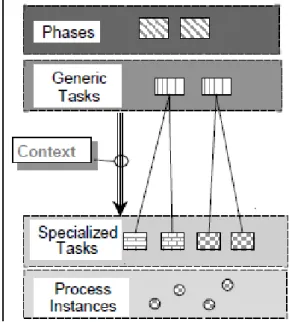
The CRISP-DM is seen as a hierarchical process model with four levels of abstraction, as presented in Figure 2.

Figure 2 - CRISP-MD Levels (Wirth & Hipp, 2000)

The first level (phases) is a combination of generic tasks (second level), and these tasks are made to be the most complete (cover the whole possibilities and processes of data mining) and stable (handle unforeseen developments) as they can. The third level aims to describe the tasks from the previous level. The last level has the objective to register all decisions, actions, and results made (Chapman et al., 1999). This life cycle is then divided into six different phases, as shown in Figure 3.

(36)

Chapter 3 - Work Methodology

16 These phases include (Wirth & Hipp, 2000):

• Business Understanding - the objective is to understand the requirements and objectives of a project and turn that into a data mining problem. This is present in Chapter 1 and 1.1 of this research.

• Data Understanding – This phase and the previous one are complementation of each other as to understand the data, one has to understand the context in which they will be used and to understand the objective of the project, one has to know what the type of data that will be used. In this research, a statistical analysis will be done to understand the data better.

• Data Preparation - After a good understand of the business and data, data preparation can start. This phase is the combination of all the necessary activities to build the final dataset, which includes attribute selection, data cleaning, construction of new attributes, and data transformation.

• Modeling - As this aims to apply different modeling techniques and parameter calibration, this phase must be done back and forth with the previous one. In this research, some of the most used algorithms found in the literature will be used.

• Evaluation - After having one or two high-quality models by using data analysis and before deploying the model, it is needed to do an evaluation of the model to prove that it can achieve the objectives proposed. To do this, the model will be assessed by using the most used metrics in the literature, such as precision, recall, accuracy, and f-measure.

• Deployment - the knowledge obtained in the model has to be presented through a report or presentation or both.

(37)

17

Figure 4 - CRISP-MD lifecycle overview Wirth & Hipp, (2000)

3.1.Business and Data Understanding

The data used for this research was from a company operating in the bank sector in Portugal (only information possible to reveal due to privacy agreement) and consisted in two excels, one with deployment tickets information and the other with incident tickets information.

The excels had pieces of information such as date of end and start of the ticket, description, who made the deployment, where was the deployment assigned, since the organization has different headquarters across the country, different categories of the application or software and time it took to end the ticket.

Both have information from 1st January of 2015 to the 28th September of 2018. The deployment file had initially 281091 entries, and 126 attributes, and the incident file had 114146 entries and 161 attributes.

The dataset did not contain information that links an incident directly to a deployment. The description given in the incident tickets is not enough to know what may have been the deployment that caused it and so the only way to relate them is by the name of the application or software.

(38)

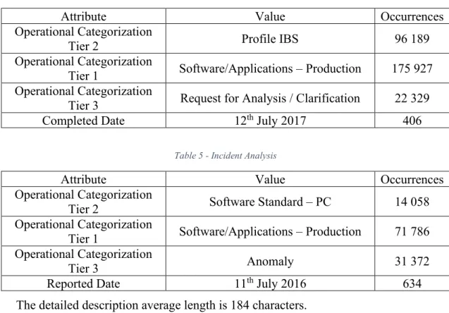
18

Table 4 and Table 5 show the value that occurred the most for each dataset in a specific attribute.

Table 4 - Deployment Analysis

Attribute Value Occurrences

Operational Categorization

Tier 2 Profile IBS 96 189

Tier 1 Software/Applications – Production 175 927 Operational Categorization

Tier 3 Request for Analysis / Clarification 22 329

Completed Date 12th_{July 2017} ₄₀₆

Table 5 - Incident Analysis

Attribute Value Occurrences

Tier 2 Software Standard – PC 14 058

Tier 1 Software/Applications – Production 71 786 Operational Categorization

Tier 3 Anomaly 31 372

Reported Date 11th_{July 2016} ₆₃₄

The detailed description average length is 184 characters.

3.2. Data Preparation

In order to achieve better results and to remove not necessary entries and attributes, several transformations were made before having the final dataset. Figure 5 shows the workflow of the transformations, which will then be further explained throughout this chapter.

3.2.1 Initial Attribute Cleaning

After the first analysis, it was taken out attributes that did not have any relevant information such as ticket ID and attributes that had repeated information of other attributes. 11 attributes from deployments and 6 from incidents were removed in this process.

(39)

19

(40)

20 3.2.2 Irrelevant Attributes

Then after checking with the company to validate the relevance of some attributes, it was decided to eliminate more attributes such as attributes that most of the entries were empty and others, such as email, phone number, breach reason, model/version and many others that both the company and the author agreed that would not bring much information.

After this, the files went from 115 attributes to 23 in the deployment’s dataset and from 155 attributes to 26 in the incident’s dataset. In this process, the start date of the deployments and the end date of the incidents were removed as they would not be needed because the intention is to relate when the deployment was made, and the incident was created.

3.2.3 Irrelevant and duplicated entries

After this, it was removed tickets entries with states other than closed to avoid having repeated tickets with only different states due to the dataset having different entries for the different states of the ticket and in the end the duplicates entries were removed.

442 entries from deployments and 1040 from incidents were removed in this process, leaving the dataset with 280649 entries in the deployment’s dataset and 113106 in the incident’s dataset.

3.2.4 Efficiency Cleaning

Then for efficiency purposes, it was removed the entries which did not have a match in the other excel making the deployment data going from 280649 entries to 199776 and the incident data from 113106 to 109652. The deployment dataset had deployments after the last incident date, making them not useful, so these were removed, there was 274 deployments in this situation, leaving the final deployment’s dataset with 199502. After the first results, it was decided to remove more attributes to see if it would make the algorithm have better results, and so ten more attributes were removed, leaving the deployments dataset with 13 attributes.

3.2.5 Attribute Creation

To perfom a prediction, it was needed to add an attribute that had the number of incidents of deployment in the following days (for this research we used 3, 7 and 10 days). After the initial results, it was decided to create another attribute that has the average incident impact for each deployment, leaving the deployment dataset with 15 attributes.

(41)

21 3.2.6 Data Transformation

The description attribute had all sort of information on it, so it was decided to categorize it based on the size of the text by comparing them with the average field size. In the end, the attribute was divided into short, medium, and long description and none.

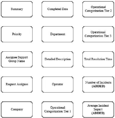
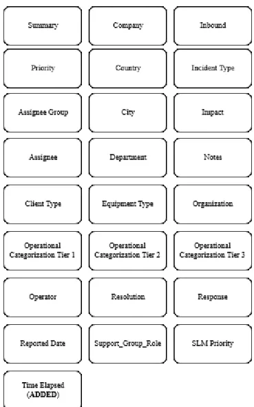
Figure6 shows the final set of attributes used from the deployment’s dataset. Figure 7 shows the final set of attributes present in the incident’s dataset.

Figure 6 - Final set of deployment attributes

• Non-Categorical Textual attributes: Summary, Detailed Description (before categorization);

• Non-Categorical Numeric attributes: Completed Date, Total Resolution Time, Number of Incidents;

• Categorical Textual attributes: Priority, Assignee Support Group Name, Request Assignee, Company, Department, Detailed Description (after categorization), Operator, Operational Categorization Tier 1, Operational Categorization Tier 2, Operational Categorization Tier 3;

(42)

22

Figure 7 - Final set of Incident attributes

For this research, the only relevant attributes used from the incident dataset was the Reported Date (Categorical numeric), Impact (Categorical numeric) and Operation Categorization Tier 2 (Categorical textual).

3.3. Modeling

It was decided to apply Naïve Bayes, SVM, RF, and CARTto measure the accuracy of the prediction. The algorithms were used with the library sklearn (Pedregosa, F., Varoquaux, G., Gramfort, A., Michel, V., Thirion, B., Grisel, O., Blondel M., Prettenhofer, P., Weiss, R., Dubourg, V., Vanderplas, J., Passos, A., Cournapeau, D., Brucher, M., Perrot, M., Duchesnay, E., 2011) in python with a validation size of 25% and 7 as seed. For the library to use the algorithm all data could not have any fields of type String or be empty, so the empty fields were filled with zeros, and the strings were categorized by using a function from the same library. The algorithm was applied to the

(43)

23

deployment file by trying to predict the number of incidents attribute that were created based on the comparison of the two datasets.

3.4.Evaluation and Results

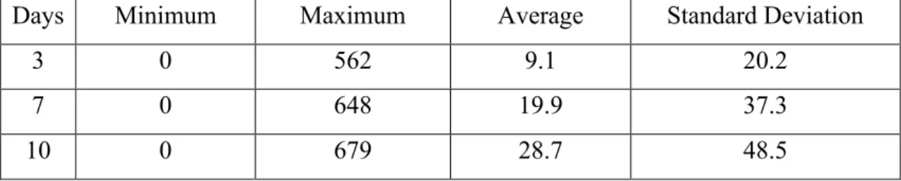
The number of incidents had the following distribution, as showed in Table 6.

Table 6 – Number of Incidents Distribution

Days Minimum Maximum Average Standard Deviation

3 0 562 9.1 20.2

7 0 648 19.9 37.3

10 0 679 28.7 48.5

As it can be seen, there is a good distribution of values, so it was decided to make different types of predictions.

• First, where the number of categories is zero, meaning that the algorithm tries to predict exactly the number of incidents.

• Second, where the number of incidents is categorized in “no accidents” and “accidents”.

• Third in “no accidents”, “below average accidents” and “above average accidents”.

• Finally, in “no accidents”, “residual accidents” (one or two), “below average accidents” and “above average accidents”.

The intention behind this categorization was not only to improve results but to understand how well the algorithms would work with different requirements, like for example, if the organization wants just to know if it has or not incidents or if it has a low number of incidents or a high number.

The author started by applying Naïve Bayes and SVM as these were the most used algorithms in the literature and then further explored algorithms such as RF and CART. After these first results, it was decided to investigate further other possible combinations, such as counting weekends and holidays, considering the average incident impact for each deployment and taking both into account.

The results for the Naïve Bayes, SVM, RF and CART algorithms are present in Table 7, 8, 9, 10 respectively, with the original results, using weekends and holidays, average impact of incidents and both.

(44)

24

Table 7 - Naive Bayes results. Original (O), Weekends and Holidays (WH), Impact (IMP)

NUMBER OF

CATEGORIES DAYS

ACCURACY (%) PRECISION (%) RECALL (%) F-MEASURE (%)

O WH IMP ALL O WH IMP ALL O WH IMP ALL O WH IMP ALL

0 3 22.9 19.5 34.1 27.4 12 10 29 21 23 19 34 27 23 11 28 22 7 15.4 14.8 20.9 20.1 6 6 16 16 15 15 21 20 8 7 16 16 10 13.1 11.4 17.8 15.6 5 3 14 11 13 11 18 16 6 5 14 12 2 3 69.8 76.2 84.5 87.8 68 74 85 88 70 76 85 88 68 75 84 87 7 80.5 80.8 90.4 90.7 79 79 90 90 81 81 90 91 79 80 90 90 10 82.7 84.0 92.2 93.1 81 83 92 93 83 84 92 93 82 83 92 93 3 3 58.9 62.5 75.8 76.3 53 58 73 74 59 63 76 76 54 58 73 74 7 62.3 62.8 74.6 74.9 57 57 71 71 62 63 75 75 57 58 71 71 10 62.5 61.5 73.4 73.0 56 55 69 68 61 62 73 73 55 55 69 67 4 3 43.8 53.0 59.2 64.7 38 47 63 63 44 53 59 65 36 46 53 60 7 56.1 56.7 65.9 66.3 51 52 62 62 56 57 66 66 51 51 62 62 10 56.2 56.4 65.3 65.3 51 48 61 60 56 56 65 65 51 50 61 60

(45)

25

Table 8 - SVM results. Original (O), Weekends and Holidays (WH), Impact (IMP)

NUMBER OF

CATEGORIES DAYS

0 3 24.3 19 24.8 19.1 24 24 26 24 24 19 24 19 10 6 10 7 7 15 14.9 15 14.9 22 23 23 24 15 15 15 15 4 4 4 4 10 13 11.3 13 11.3 25 17 26 20 13 11 13 11 3 3 3 3 2 3 62.7 72.8 62.7 72.8 66 76 69 77 63 73 63 73 49 62 49 62 7 79 79.3 79.1 79.3 82 82 83 83 79 79 79 79 70 70 70 70 10 82.7 85.2 82.7 85.2 86 87 86 87 73 85 83 85 75 79 75 78 3 3 52.7 58.1 52.8 58.2 57 65 61 67 53 58 53 58 37 43 37 43 7 60 60.5 60 60.5 69 70 69 71 60 60 60 60 45 46 45 46 10 60.4 61.8 60.4 61.8 72 74 72 74 60 62 60 62 46 48 46 48 4 3 31.7 42.9 31.7 42.9 48 59 51 62 32 43 32 43 16 26 16 26 7 49 49.7 49 49.7 63 66 65 66 49 50 49 50 33 34 33 34 10 52.2 55.4 52.3 55.4 70 71 71 73 52 55 52 55 36 40 36 40

(46)

26

Table 9 - RF results. Original (O), Weekends and Holidays (WH), Impact (IMP)

NUMBER OF

CATEGORIES DAYS

0 3 44.5 41.5 58.8 54.8 41 39 57 54 45 41 59 55 42 40 57 54 7 41.1 44.7 52.5 52.3 39 43 51 51 41 45 52 52 40 43 51 51 10 40.2 42.9 49.4 50.3 38 41 48 50 40 43 49 50 39 42 48 49 2 3 84.2 91.1 90.4 94.2 84 91 90 94 84 91 90 94 84 91 90 94 7 93.9 94.2 96 96.1 94 94 96 96 94 94 96 96 94 94 96 96 10 95.1 96 97 97.5 95 96 97 98 95 96 97 98 95 96 97 98 3 3 76 82.2 89.6 91.9 76 83 89 92 76 82 90 92 75 82 89 92 7 83.8 84.5 92.6 93.2 84 85 93 93 84 85 93 93 83 84 92 93 10 85.6 89.1 93.6 95.4 86 89 94 95 86 89 94 95 85 89 93 95 4 3 60.9 72.3 74.5 82.6 61 72 75 83 61 72 75 83 61 71 75 82 7 78.9 79.1 86.7 87.5 79 79 87 88 79 79 87 88 78 78 86 87 10 80.7 84.1 88.9 91.7 80 84 89 92 81 84 89 92 80 84 89 92

(47)

27

Table 10 - CART results. Original (O), Weekends and Holidays (WH), Impact (IMP)

NUMBER OF

CATEGORIES DAYS

0 3 86 85.4 91.2 89.9 86 85 91 90 86 85 91 90 86 85 91 90 7 86.5 86.5 89.5 88.5 87 87 90 89 87 87 89 89 87 87 89 89 10 86.7 84.3 89.2 88.4 87 84 89 88 87 84 89 88 87 84 89 88 2 3 95.1 95.9 96.2 96.7 95 96 96 97 95 96 96 97 95 96 96 97 7 96.7 96.7 97.1 97.2 97 97 97 97 97 97 97 97 97 97 97 97 10 96.4 97 97.5 98.1 96 97 97 98 96 97 97 98 96 97 97 98 3 3 91.2 93 97.4 98.8 91 93 97 99 91 93 97 99 91 93 97 99 7 94.8 94.8 99.1 99 95 95 99 99 95 95 99 99 95 95 99 99 10 96.3 96.8 99.2 99.5 96 97 99 99 96 97 99 99 96 97 99 99 4 3 89.5 91.2 94.2 96 90 91 94 96 89 91 94 96 89 91 94 96 7 93.2 92.7 96.7 96.7 93 93 97 97 93 93 97 97 93 93 97 97 10 94 95 96.9 97.5 94 95 97 97 94 95 97 97 94 95 97 97

(48)

28

Table 11 - Algorithms best accuracy results comparison

NUMBER OF CATEGORIES DAYS NAÏVE BAYES (% ACCURACY) SVM (% ACCURACY) RF (% ACCURACY) CART (% ACCURACY) 0 3 34.1 24.8 58.8 91.2 7 20.9 15 52.3 89.5 10 17.8 13 50.3 89.2 2 3 87.8 72.8 94.2 96.7 7 90.7 79.3 96.1 97.2 10 93.1 85.2 97.5 98.1 3 3 76.3 58.2 91.9 98.8 7 74.9 60.5 93.2 99.1 10 73.4 61.8 95.4 99.5 4 3 64.7 42.9 82.6 96 7 66.3 49.7 87.5 96.7 10 65.3 55.4 91.7 97.5

To evaluate the results, it was used accuracy, precision, recall, and f-measure. The precision-recall and f-measure are the weighted averages of each category, meaning it considers the number of samples of each category.

As it was used cross-validation to obtain the results, the results in the table are an average of the results calculated by cross-validation, these results have an average standard deviation of 1.2%.

The weekends and average impact of incidents had in most cases a good impact on results, improving in some cases the results by 22%.

Overall CART was the algorithm with the best results. Having 2 categories is the one that manages to get better results, and overall using 10 days gap to relate deployments and incidents gets the best results also, except for when the number of incidents is not categorized, but further analysis will be given on the next chapter.

3.5.Deployment

To present the work that was made on the model and to show how the model can be used, it was made apart from this document, documentation for the organization from which the data was used, and a demo, shown in Figure 8, to show how a future implementation would look and how it could work. The values shown in this picture are just an example of what would appear.

In this prototype, the person has completed the development and is ready to deploy, in which the deployment information is inserted, either manually or automatically, which will be used by the algorithm to make the desired prediction and later be used to improve the accuracy of the prediction of later deployments. The person who makes the

(49)

29

deployment can then choose the type of prediction he or she wants (the exact number of incidents, will or will not have incidents, will not have incidents, below average or above average or will not have incidents, just one or two, below average and above average). After this, the system would then show the user the prediction that it was made based on the information that was given, in this case, it was the number of incidents, as well as the level of confidence to which he is predicting. This level of confidence would be the accuracy shown in the previous chapter, and so it would not be the level of confidence related to that specific prediction, but to the overall accuracy of the algorithm.

Figure 8 - Implementation demo design

Depending on both results the person can then rethink and give a better look to the deployment or give a heads up to his or her manager that there is a probability of an incident after that deployment is made.

(50)

(51)

31

Chapter 4 – Discussion

In this chapter, a detailed analysis is done, first going through each algorithm overall, analysing which one performed better and worse, then discussing why some combination of parameters (days and categories) worked better than others overall and analyse the impact that taking into account the weekends, holidays and average impact had.

As shown in the previous chapter, the best result came from CART with 99.5% when setting the number of incidents over 10 days and by categorizing them in 3 categories. This means that the algorithm can differentiate very well between having no incidents, a small number of incidents (below average) and a high number of incidents (above average).

Although this was the best result, CART can overall predict very well with any combination of categories and days, having very good results even when not categorizing the number of incidents meaning that the algorithm is even able to predict with great accuracy the exact number of incidents that a deployment can have.

As the results show, RF also performs well, which demonstrates that decision trees algorithms work very well with this type of data probably because these are better at dealing with outliers and with nonlinear attributes.

Naïve Bayes had average results with 3 and 4 categories, good results with 2 categories and bad results with no categories. Naïve Bayes was the most used algorithm in the literature, but in this research, it did not perform as well as it was expected and ended up being surpassed by the decision trees algorithms. Still, as said previously, it is still a viable algorithm to use to predict if deployment will have or not an incident.

SVM had overall bad results and the worse of the four algorithms, this might be related to how SVM works, as in the end the data that was used had a small number of textual parameters and ended up being more categorical data.

As for the combination of parameters, first, the intention to use a different number of categories was to understand with how much detail the algorithms were able to predict, as, for the number of days, the intention was to understand the span in which the incidents correlate with the deployments.

Having said that and by analyzing the results, when we categorize the number of incidents the span that has the best results is the 10 days span, but when we do not categorize the incidents the 3 days span gets the best results. This may indicate that when we categorize and use a long span of days (such as 10 days), there is a higher probability

(52)

Chapter 4 - Discussion

32

that most of the number of incidents will fall into one category, leading to an overfit of the results. This means that the algorithm will think it is safer to guess that the deployment will have incidents or a specific number of incidents. When we do not categorize incidents, this does not happen because each deployment will have a different number of incidents and will not fall all in the same category.

So, in the end, despite the 10 days span having better results (by a small margin), the 3 days span represent better in which an incident is actually related or created by a deployment.

As for the categories, as it was expected, having no categories ends up in having worse results, despite the good results with the CART algorithm. Having only two categories maximizes the results with the exception of the CART algorithm. As stated previously, the intention with the categorization was not only to maximize the results, but to understand the level of detail the algorithm is able to predict in order to deliver different type of analysis (will or will not have incidents, will it have small number of incidents or a great number of incidents or even just one or two incidents).

Finally, as said in the previous chapter, taking into account the weekends, holidays and average impact of incident improved the results with a few exceptions such as the weekends and holidays giving worse results when not categorizing the number of incidents for the same reasons as having a larger day span also gives worse results. The average impact of the incidents in most cases improved the results, except for SVM, where it had no impact on the results. The reason could be the same as to why SVM has the worse results of all algorithms used, since the impact is just another statistical/categorical parameter, it does not add much to the SVM algorithm.

(53)

33

Chapter 5 – Conclusions

Overall the results allow us to predict if a certain type of deployment with certain types of attributes has a high or low probability of having incidents, by raising awareness of the deployment team to be more careful when doing the deployment. Although it does not have the best accuracy on guessing the exact number of incidents, it does have a good accuracy when deciding if a certain deployment has or not an incident and even when predicting if it will have just a few or around the average incidents which allow once again the deployer to have a better trust when deploying the application or software.

It was also found out that the decision tree algorithms such as RF and CART work very well with this type of data.

RQ1 - Can software deployments information be used to predict incidents?

Grounded on the achieved results, it is feasible to argue that it is possible to use software deployment information to predict incidents with some accuracy. Greater accuracy can be achieved if we do not need to know the exact number of incidents, but instead, we just want to know if it will or will not have incidents, or if it will have a small or high number of incidents.

To wrap the conclusions, these were the main conclusions from this research:

• Assuming that each incident is related with each deployment made in a certain day span, it is feasible to predict the number of incidents with some accuracy event with low to no detail on what was done on the technical level;

• Decision Tree works very well with this type of data;

• On the professional outcome, this information can be used not only to prevent and better allocate resources for future incidents but may be used as an overall measurement tool as well, as the better the teams work, the fewer incidents the system will predict;

• On the academical outcome, this study allowed to understand which algorithm is better with this type of data, as well as, showing one of the possible ways to predict incidents with small to no information of the technical side of the deployment.

5.1. Research Limitation

As previously stated, specific information that enabled us to associate an incident directly was not provided by the organization, although this type of information would

(54)

Chapter 5 - Conclusions

34

not guarantee better results, since it is very difficult to always guarantee that a specific incident ticket is related to a specific deployment.

Plus, the deployments’ information did not specify much of what was done in the deployment on the technical side which could have improved the results since most of the incident prediction that was found in the literature was based on technical information of the deployment.

5.2. Future Work

As said before this study worked with some unique type of data and so it served as a foundation for more studies to be done. The next paragraphs are a list of what can be done to complement this study.

Improve and add some of the attributes, like categorizing descriptions, adding the importance of the deployment, give more detail of what was done on the technical level. and then check if the results improve with that.

An implementation of this study as a Decision Support System to help managers understand what is the type of deployments that have more incidents, to understand if the number of incidents is getting worse or better and allowing them to act better and faster on possible future incidents.

This study can also be used to know the impact that is having a prediction of the incidents can have on the processes. How does it impact them? A good way to measure this is to run the algorithm daily and see if the number of incidents predicted goes up or down. Since with the use of this study, there will be bigger attention when doing a deployment, hopefully a decrease in the number of incidents will happen and the daily prediction will actually go down and so it can be use to evaluate the impact of the study.

(55)

35

Bibliography

Aguiar, J. F. F., Pereira, R., Vasconcelos, J. B., & Bianchi, I. (2018). An Overlapless Incident Management Maturity Model for Multi-Framework Assessment (ITIL, COBIT, CMMI-SVC). Interdisciplinary Journal of Information, Knowledge, and Management, 13, 137–163. https://doi.org/10.28945/4083

Altintas, M., & Tantug, A. (2014, September). Machine learning based volume diagnosis. Proceedings of the International Conference on Artificial Intelligence and Computer Science (AICS 2014). 195–207.

Bari, A., Chaouchi, M., & Jung, T. (2014). Predictive analytics for dummies. Hoboken, NJ: John Wiley & Sons, Inc.

Bartolini, C., Salle, M., & Trastour, D. (2006). IT service management driven by business objectives An application to incident management. 2006 IEEE/IFIP Network

Operations and Management Symposium NOMS 2006, 45–55.

https://doi.org/10.1109/NOMS.2006.1687537

Bartolini, C., Stefanelli, C., & Tortonesi, M. (2010). SYMIAN: Analysis and performance improvement of the IT incident management process. IEEE Transactions on

Network and Service Management, 7(3), 132–144.

https://doi.org/10.1109/TNSM.2010.1009.I9P0321

Bishop, C. M. (1996). Neural Networks: A pattern recognition perspective. Neural Computing Research Group Aston University, Birmingham, UK. 23.

Brownlee, J. (2016). Machine Learning Mastery With Python. (1st Ed). 179.

Çalikli, G., Staron, M., & Meding, W. (2018). Measure early and decide fast: transforming quality management and measurement to continuous deployment. International Conference on Software and System Processes, 51–60. https://doi.org/10.1145/3202710.3203156

Catal, C. (2011). Software fault prediction: A literature review and current trends. Expert

Systems with Applications, 38(4), 4626–4636.

https://doi.org/10.1016/j.eswa.2010.10.024

Chapman, P., Clinton, J., Kerber, R., Khabaza, T., Reinartz, T., Shearer, C., & Wirth, R. (1999). Step-by-step data mining guide. 76.

Dearle, A. (2007). Software Deployment, Past, Present and Future. Future of Software Engineering (FOSE ’07), 269–284. https://doi.org/10.1109/FOSE.2007.20 Duda, R. O., Hart, P. E., & Stork, D. G. (2001). Pattern classification (2nd ed). New

York, NY: Wiley.

Forte, D. (2007). Security standardization in incident management: the ITIL approach.

Network Security, 2007(1), 14–16.

https://doi.org/10.1016/S1353-4858(07)70007-7

Fronza, I., Sillitti, A., Succi, G., & Vlasenko, J. (2011). Failure Prediction based on Log Files Using the Cox Proportional Hazard Model. SEKE 2011 - Proceedings of the 23rd International Conference on Software Engineering and Knowledge Engineering, 456–461.

Fulp, E. W., Fink, G. A., & Haack, J. N. (2008). Predicting Computer System Failures Using Support Vector Machines WASL'08 Proceedings of the First USENIX conference on Analysis of system logs, 5-5.

Gacenga, F., Cater-Steel, A., Tan, W.-G., & Toleman, M. (2010). IT Service Management: Towards a Contingency Theory of Performance Measurement. Service Science, 19.