Changing Returns to Education in Portugal During the 1980s and Early 1990s: OLS and Quantile Regression Estimators

Changing Returns to Education in Portugal During the 1980s and Early

1990s: OLS and quantile regression estimators

Joop Hartog * Pedro T. Pereira** José A. C. Vieira ***

Abstract

This paper examines the evolution of the returns to education in Portugal over the 1980s and early 1990s. The main findings indicate that the returns to education have increased, particularly after joining the European Union in 1986. Since this occurred along with an increase in the level of education within the labour force, the process is most likely demand driven. The results also indicate that modelling on average (i.e. OLS) misses important features of the wage structure. Quantile regression (QR) analysis reveals that the effect of education is not constant across the conditional wage distribution. They are higher for those at higher quantiles in the conditional wage distribution. Wage inequality expanded in Portugal over the 1980s and the returns to education had an important role in this process.

Keywords: returns to education, quantile regression JEL codes: C13, J31

* University of Amsterdam and Tinbergen Institute

Address: Roetersstraat 11, 1018 WB Amsterdam, The Netherlands E-mail: hartog@fee.uva.nl

** Universidade Nova de Lisboa

Address: Tv Estêvão Pinto, 1070 Lisboa, Portugal E-mail: ppereira@feunix.fe.unl.pt

*** Universidade dos Açores and Tinbergen Institute Address: Rua Mãe de Deus, 9500 P. Delgada, Portugal E-mail: jvieira@alf.uac.pt

The authors thank Hessel Oosterbeek and Athula Ranasinghe for their comments on earlier versions of this paper. Financial support from program PRAXIS XXI under grant PRAXIS/2/2.1/CSH/781/95 and FEDER is acknowledged. The third author also acknowledges financial support from program PRAXIS XXI under grant BD/3486/94 and from the University of the Azores.

1 Introduction

In the first half of the 1980s Portugal experienced a severe economic crisis. However, after the mid-1980s the economy grew at a fast pace and employment expanded, with the labour market functioning at nearly full-employment. This was a period during which the country experienced trade changes due to joining the European Union (in 1986) and embarked upon a path of modernisation of the industrial structure, namely through the introduction of new production technologies. It is also well documented that wage inequality increased substantially during this period (Cardoso, 1997, Vieira et al., 1997).

In view of such economic changes, it certainly would be interesting to observe possible changes in the rates of return to education during this period. It is worth mentioning that factors such as increased openness of the economy leading to importation of labour intensive manufactured goods (thus reducing the domestic demand for low-educated workers), or the use of technology complementary with highly educated labour have been indicated as factors behind the rise of the returns to education, and ultimately increased inequality in the U.S. over the 1980s (see e.g., Wood, 1994, and Berman et al., 1994). Contrary to the U.S. experience, the increased openness of the Portuguese economy is with more developed countries after joining the European Union (EU). Within the EU the country has comparative advantage in labour-intensive sectors requiring low-educated labour (Courakis, 1991). This would suggest an increase in the demand for low-educated rather than for highly-educated labour in the post-integration period. Nevertheless, this may have been counteracted by other factors. First, structural funds from the EU in combination with specific financial aids to industrial investment for modernisation of the productive structure have contributed to the introduction of new technologies. Second, the liberalisation of trade with more developed countries producing capital goods likely encouraged the importation of technology requiring skilled labour.

The paper collects comparative empirical evidence on the evolution of the returns to education in Portugal. Particularly, it examines the years of 1982, 1986 and 1992. This time period is important since it captures the situation 4 years before joining the EU, the situation at the time of joining the EU and the situation 6 years later. For this purpose, we use the same data source and the same estimation procedures over the period to be examined. Obviously this is a desirable property to make intertemporal comparisons.

For empirical purposes, we make use of ordinary least squares (OLS) and quantile regression (QR) estimators. The latest estimator allows us to assess how the effect of education varies across the whole conditional wage distribution. In the OLS perspective, the regression coefficients are assumed constant across the entire conditional distribution. However, there is no specific reason to assume in advance such uniformity. The characterisation of the conditional expectation (mean) likely constitutes only a limited aspect of the wage distribution. Indeed, recent studies suggest that restricting the analysis to average effects misses important features of the wage structure (e.g. Buchinsky, 1994, Chamberlain, 1994, Machado and Mata, 1997, Fitzenberger and Kurz, 1997). This paper also supports this view.

The paper is organised as follows. The next section presents a brief description of the Portuguese education system and educational attainment of the population. Section 3 describes the estimation methods. Section 4 includes some theoretical background and motivates the use of the QR technique. Section 5 describes the data set. Section 6 includes the estimation results. First, we estimate a standard human-capital wage equation. Then, a spline in years of education is considered in order to capture differences in returns to education between educational levels.

Finally, we present results for a wage equation that captures the worker-job matching wage effect (ORU equation). Section 7 deals with returns to education and wage inequality. Finally, section 8 concludes and summarises.

2 Education in Portugal

The current education system in Portugal is composed of primary, secondary and tertiary education. Compulsory education has been established at a quite low threshold. Completion of the first three years of education corresponded to the compulsory level of education until 1956, when it was established at four years.1 _{It increased to six years in 1964 and to nine years after} the mid-1980s.

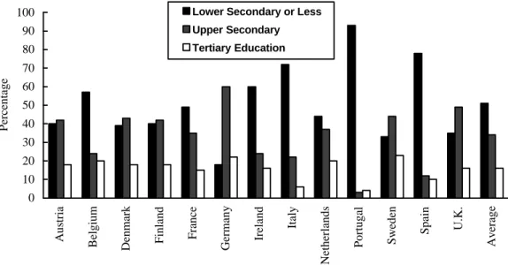
--- insert Figure 1 about here

---As shown in Figure 1, Portugal has an incredibly low level of education in a European perspective. Because of this, the country has been recently a terrain of intense efforts aimed to augment the education level of the population. Typical examples are the extension of the compulsory level of education, curricula diversification, and expansion of the network of education and training institutions. In particular, university education expanded significantly after the mid-1980s largely due to the emergence of private universities. The average years of education within the labour force passed from 5.06 in 1982 to 5.98 in 1992 (see Vieira et al., 1997).

3 Estimation methods

Ordinary least squares is one of the methods used in this analysis. This method allows us to estimate the effect of education on the mean of the conditional wage distribution. However, the impact of education on the mean of that distribution likely describes a partial aspect of the statistical relationship among variables. In such a case, it may be important to examine that relationship at different points of the conditional distribution function. Quantile regression (QR) warrants such an analysis. The QR method was introduced by Koenker and Basset (1978). They define the θth regression quantile as the solution to the problem:

min β∈Rk _{i y x}θ_β yi xiβ _{i y xβ} θ yi xiβ i i i i − + − −         ≥ <

∑

∑

This is normally written as:

min ( ' ) β ρ_θ β ∈ −

∑

where ρ ε_θ( ) is the check function defined as    < − ≥ = 0 if ) 1 ( 0 if ) ( ε ε θ ε θε ε ρθ

The model specifies the θth-quantile of the conditional distribution of the log wages given the covariates x as ) 1 , 0 ( , x ) x | ( Q_y θ = 'β_θ θ∈ (2)

By variation of θ, different quantiles can be obtained. The least absolute deviation (LAD) estimator of β is a particular case within this framework. This is obtained by setting θ=0.5 (the median regression). The first quartile is obtained by setting θ=0.25, and so on. As we increase θ from 0 to 1 we trace the entire distribution of y, conditional on x. This problem does not have an explicit form, but can be solved by linear programming methods. In the present study it is solved by linear programming techniques suggested in Amstrong et al (1979). In practice, obtaining standard errors for the coefficients in quantile regression is a difficult problem and one for which the literature provides only a sketchy guidance. In the present study, we used a bootstrap method with 20 repetitions.

4 Some theoretical background

In order to clarify the importance of the QR technique in a specific context, we present a modified version of the model of optimal schooling choice developed in Card (1994). Assume that an individual chooses education and maximises a utility function of the type:

U w E( , )=lnw−rE

(3)

subject to the individual’s opportunity set summarised by w=g(E), representing the level of wages (w) available at each level of education (E). This type of utility function derives naturally by assuming that the individual maximises the discounted present value of wages, discounts the future at a rate r, and earns nothing while in school (see Willis, 1986, Card, 1994). The first order condition for optimal education requires that:

g E g E r

' ( ) ( ) =

(4)

In the optimum the marginal rate of return equals the marginal cost of the investment in education.

To make the model empirically operational, we must choose functional forms for the marginal (proportional) benefits and costs of education. For simplicity, it is assumed that the marginal costs are increasing functions of the amount invested in education and that the marginal returns do not vary with education (the latter assumption is only a matter of simplicity and can be discarded without changing the main implication). Specifically,

g E g E r r kE i i ' ( ) ( ) = = + β (5)

As the individual invests in education until the point where marginal costs equal marginal benefits his optimal amount of education is given by:

E r k i i i * ₌ β − (6)

Integration of the marginal benefits in (5) leads to a log-linear wage equation for individual i of the type:

ln wi = +ai βiEi

(7)

Traditionally, variation in ability concerns variation in the intercept of the wage equation. One appealing feature of the model is that variation in ability also concerns the slope. In other words, ability influences the wage-effect of education. If it only influenced the intercept, individuals with higher ability might well invest less in education, since they have higher opportunity cost of school attendance.

The model identifies two sources of heterogeneity in the population: variation in marginal rates of return to education at each level of schooling (loosely differences in ability) and variation in the marginal costs of investment in schooling (loosely differences in access to funds or tastes for education). Except under very restrictive assumptions, equilibrium in this model implies a non-degenerate distribution of marginal returns to education across the population (Card, 1994). Such a distribution introduces some ambiguity into the interpretation of the causal effect of education: in essence each person has his own causal effect.

This simple model raises an important conceptual question on empirical work. If individuals have different returns to education at the same level of schooling there is no unique causal effect of schooling on wages. The quantile regression technique allows us to shed some light onto the issue. The estimation of the effect of education on conditional quantiles permits to uncover individual heterogeneity in the effect of education on wages. Two examples based on Koenker and Basset (1982), Manski (1988) and Mata and Machado (1995) may help to clarify this point.

Aside from other covariates, consider the following simple wage equation:

ln w_i = +a βE_i+ε_i (8)

In this equation one can define ai=a + εi where εi are i.i.d random terms. Given that

specification (8) is correct, heterogeneity among individuals only affects wage levels and therefore concerns the intercept of the wage equation. In such a case,

Qlnw( | )θE =[a+Qε( )]θ +βE, θ∈(0, 1)

(9)

Only the intercept differs for different conditional quantiles. The slope - i.e. the marginal effect of E - will be invariant to the quantile being estimated. The (theoretical) conditional quantile functions constitute a family of parallel lines. They would also be parallel to the mean regression line: only the conditional location of the dependent variable would change for different values of θ. In such a case, there would be no substantial losses of information, with respect to the slope, by estimating solely a measure of conditional central tendency such as the mean (estimated by OLS).

However, Koenker and Basset (1982) alert that when errors are not identically distributed the situation is different. Probably in many applications the conditional quantile function

Q_y( | )θ x does not depend upon x only in location because the exogenous variables may also influence the scale, tail behaviour, or other characteristics of the conditional distribution of y (see Koenker and Basset, 1982, p.49). In such cases, the slope coefficients depend in a non-trivial way on θ and one might expect to find discrepancies in the estimated slope parameters at different quantiles. To clarify the importance of this point consider the (random coefficient) model

ln w_i = +a_i b E_{i i}

(10)

where ai=a + εi and bi=b + εi and εi is a random variable reflecting individual heterogeneity.

In this case, the intercept and the slope coefficient of the theoretical conditional quantile line will vary with the quantile being estimated. If the ‘ability’ effect concerns only the slope of the wage function (i.e. ai=a for all individuals), as in most of Card’s (1994) set-up, then

Q_lnw( | )θ E = +a [b+Q_ε( )] .θ E In any case, bi= b + εi, captures the idea that wages are

heterogeneously determined and that the slope coefficient differs in observations with the same observed education. Therefore, there may be information gains from estimating and comparing several conditional location measures for the dependent variable, even after controlling for a large set of observed individual and job characteristics. We will do that for our Portuguese data set, both overall and for several decompositions.

5 Data source

The data used here were drawn from Quadros de Pessoal for the years of 1982, 1986 and 1992. All firms with wage earners must complete a standardised questionnaire every year and send it to the Department of Labour. The data refer to March of each year and include information on individual workers such as age, tenure with the current firm, the highest completed level of education, and gender. Information is also available on firm size, industry, region, bargaining regime, firm ownership structure, job complexity and hours worked. It also includes information on workers’ monthly wages. Years of education were determined by imputing the nominal number of completed years in order to complete the level reported in the data. Potential labour market experience was computed as age minus years of education minus six. Data on firm age were gathered from an external file used in MESS-DE (1994). Civil servants and people serving in the armed forces are not included in the data source. Records

with missing values were deleted from the original samples, as were part-timers, the self-employed, unpaid family workers, agricultural workers, fishermen, and apprentices. Observations in which tenure was greater than labour market experience were also deleted. The final sample includes 57737, 57299 and 54307 individual observations in 1982, 1986 and 1992, respectively.

6 Estimation results

6.1 Including years of education in the regressors list

This section includes the results of a Mincer-type wage-equation, where the individual’s years of education are used as an explanatory variable. Other covariates are a vector of ones, years of tenure with the current firm, a third polynomial for experience, and controls for hours worked, firm size, firm age, blue-collar job, gender, region, bargaining regime and industry. The dependent variable is the logarithm of monthly gross wages. The main goal is to estimate the parameter associated with years of education (i.e. the return to education, see Mincer, 1974).

The interpretation of the quantile regression coefficients is conceptually quite analogous to OLS regressions. In OLS case, the regression coefficients measure the influence of the regressor variables on the conditional mean of the dependent variable, whereas in the quantile regression case the coefficients βθ represent the influence of the regressors on the conditional θ-quantile of the dependent variable.

The marginal effect of a variable on a specific conditional quantile of the dependent variable can be obtained by the corresponding partial derivative. Therefore, ‘quantile rates of return to education’ are given by:

r Q x E w θ =∂ ln_∂ θ × ( | ) 100 (11)

The value is multiplied by hundred to give a percent interpretation.

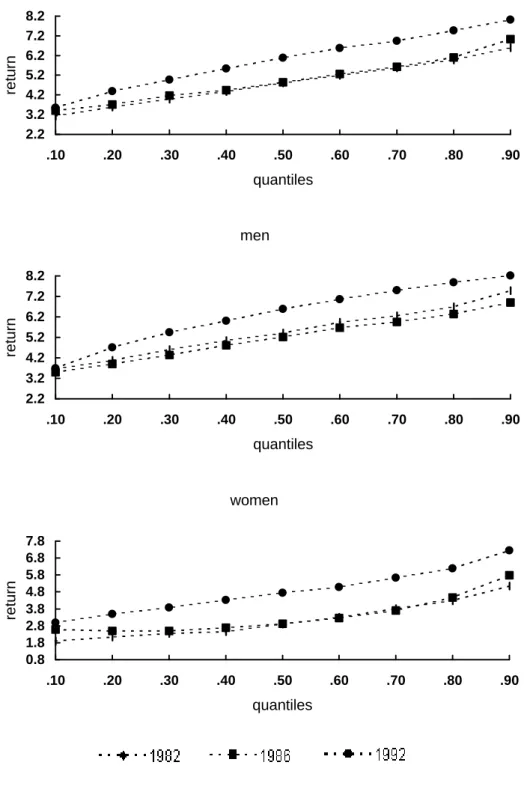
Nine quantile regressions were computed for each of the three years being examined. Furthermore, the regressions were performed for the full sample, and for two sub-samples of men and women separately. Quantile rates of return to education for the present specification of the wage equation are in Table 1 in the appendix. These are plotted against the quantile numbers in Figure 2. The effect of education on wages is positive and statistically different from zero at each of the quantiles analysed. This suggests that wages increase all over the conditional distribution range with education. However, education affects wages differently at different parts of that distribution. It has a larger effect at higher quantiles. This is very clear for men in all three years. The same is visible for the full-sample but here men influence the pattern. Indeed for women the returns show a quite flat pattern in 1982 and 1986 until nearly θ =0.40. They apparently increase after this point. This suggests that there is heterogeneity in the returns to education, which are larger for individuals at higher (with better-unobserved earning capacity) quantiles of the conditional wage distribution. Both for men and for women, the returns to education at the 0.90 quantile are roughly double the returns at the 0.10 quantile.

-insert Figure 2 about here

---Now, let’s consider the changes over time. The pattern of change over time shows great similarities across almost all quantiles. The returns were quite stable from 1982 to 1986 (a little upward shift is visible at θ=0.90, however). There is a clear upward shift from this time to 1992. This occurred for both men and women and at almost all quantiles. The only clear exception is at θ=0.10 where there is practically no change. As a result, the difference of the effect of education at the two extreme deciles of the conditional distribution widened, and naturally contributed to increase wage inequality. In 1982, the difference in the returns between the 9th and the 1st deciles amounted to 3.48, 3.40 and 3.23 percentage points for the pooled sample and for the sub-samples of men and women, respectively. In 1992, the figures were 4.47, 4.53 and 4.27, respectively.

It is also clear that the effect of education on wages is lower for women than the corresponding values for men. This is verified across the whole distribution. However, the difference narrowed remarkably from the mid-1980s to 1992 as a result of a faster increase in the returns for women. This is also true in the OLS estimation (see Table 1 in the appendix).

6.2 Including a spline in years of education

It has frequently been observed that the returns to an extra year of education are not identical across levels (or types) of schooling. In particular, the surveys by Psacharopoulos (1985, 1994) indicate that returns are highest for primary education. From secondary to tertiary education they many increase, thus producing a U-shaped pattern.

This section changes the wage equation specification through the inclusion of a spline in years of education at three categories of the school system. This enables the effects of education on wages to vary at each of the three education categories. The coefficients on the splines are interpreted in the same way as a coefficient in a continuous education variable. The education variable is defined as follows:

education tertiary 11 x , 11 x 11 x , 0 E education ondary sec 11 x , 5 11 x 6 , 6 x 6 x , 0 E education primary 6 x , 6 6 x 0 , x E ter sec prim    ≥ − < =      > ≤ < − ≤ =    > ≤ ≤ = (12)

where x denotes the number of years of education completed by the individual.

The results are in Tables 2 to 4 in the appendix. They are also plotted in Figures 3 and 4. The main purpose of Figure 3 is to compare returns to education within a given year. Changes over time are better visualised in Figure 4.

Figure 3 shows that the rates of return tend to increase with the level of education. They are particularly high for tertiary education as compared with the other two levels. This pattern is verified across almost all quantiles and the two gender groups. That pattern of higher returns as one moves up on the education distribution is also verified for the mean (i.e. OLS) regression (see Tables 2 to 4 in the appendix). In particular, the low rate of return for years of primary education is remarkable in view of the general pattern observed by Psacharopoulos noted above. The high rate of return for primary education in these surveys, mostly refers to developing countries, as in developed countries there are no observations without primary education. An explanation may be that returns years of primary education in developing countries include the big effect of really basic education, generating literacy, whereas in the Portuguese case the results apply to the more advanced years. Still, some suspicion is warranted, as among the older generations in Portugal literacy was not attained by every individual.

insert Figure 3 about here

---For men, the returns in primary and secondary education tend to increase with the quantile numbers. The same holds for women except in secondary education in 1986. In this case they are stable, or show a mild decrease, until about θ=0.40 and then increase afterwards.

The returns to tertiary education show an inverted U-shaped, or stable, pattern as one moves up in the wage distribution. They tend to increase until the about the conditional median and to decrease after that. There are differences by gender, however. That pattern is not verified for women. In this case, the effect of a year of tertiary education is larger at higher quantiles in 1982 and 1986. However, the pattern changed drastically in 1992. In this year, the returns are very similar across all quantiles.

--- insert Figure 4 about here

---Figure 4 reveals the evolution of the returns to education at each of the three levels of education. During the 1982-86 period, returns to tertiary education remained almost unaltered for male workers. We already noted an upward shift for women, however. They increased substantially from 1986 to 1992 for men and for women at all quantiles. The changes are much more pronounced for women than for men, (indeed this is true for all three education levels). The increase for women within tertiary education is spectacular. From a quite low return as compared with men in 1982, the difference vanished by 1992. Another, particular feature for women is that the relation between return to education and the quantile numbers flattened out over time. This is due to a faster increase of the return at low than at high quantiles from 1986 to 1992.

The evolution of the returns within primary and secondary education also deserves some comments. They are characterised by a great stability between 1982 and 1986. There were upward changes after this period. In primary education, these changes were modest for men as compared with those registered for women. Indeed, for men, changes were quite mild. In secondary education, there is no alteration until θ=0.20 and at θ=0.90, for men. A small upward change apparently occurred between these points. For women, the changes were more impressive. An increase occurred between 1986 and 1992, but this becomes more salient as we move up to higher quantiles, i.e. the returns fanned out (although there is no apparent change until θ=0.20).

In summary, within primary and secondary education, we find again that the returns to an extra year of education at the 0.90 quantile are roughly double that at the 0.10 quantile and this pattern is stable over time. For men, there is modest variation of returns by quantile within tertiary education. For women, the top-to-bottom ratio of returns was about 1 to 2 in 1982 and 1986, but in 1992 there was modest variation, i.e. a convergence to the pattern found for men.

6.3 Job-worker matching and the returns to education

In this section we extend the wage equation by considering the role of job requirements for wage formation. In the standard human capital model this is superfluous. The theory implicitly assumes that each individual will get a proper job given his amount of human capital making the job requirement redundant. In such a case, education would have a unit-price characteristic throughout the labour market regardless of the job in which the individual ends up. However, assignment models pioneered by Tinbergen (1956) and followed by Sattinger (1980) and Hartog (1981, and 1986) combine individual and job characteristics and stress the existence of an assignment problem in the labour market. In this setting, the price of a specific labour characteristic is not expected to be uniform across the economy. It will be the outcome of two distributions: one applying to the supply side of the market and one referring to the demand side. The labour market system equals the two frequency distributions, with wages as the instrument. The price will depend on the allocation that is realised, which is determined by the entire distribution of demand and the entire distribution of supply of the respective characteristic.

This section has as background the assignment literature. For empirical purposes, we estimate a wage equation as suggested by Duncan and Hoffman (1981). Although this equation has no immediate representation in the existing assignment models, it reminds of this theory (see Hartog, 1997). Indeed, it constitutes a simple way to relate the supply and the demand for education. In this specification, years of education attained by the worker (Ea) are split into years of education required for the job (Er), years of education above the job requirement (Eo) and years of education below the job requirement (Eu), where:

r a o E E E = − if Ea >Er, 0 otherwise and (13) a r u E E E = − if Er>Ea, 0 otherwise

By definition, the equalityEa =Er +Eo −Eu must hold.

Hartog and Tsang (1987), Hartog and Oosterbeek (1988), Sicherman (1991), and Alba-Ramirez (1993) also used this equation. For easy reference, it was called by Hartog (1997) as the ORU specification, for Over-Required and Undereducation.

A condition to apply this specification is that workers must be classified according to the education actually completed and jobs must be classified according to the education required. This type of information is included in our data. Workers are classified according to the maximum level of education actually completed. Jobs are classified according to their requirements, since firms have to provide information to the Labour Office on the requirements

of the job performed by each individual worker. This is ranked on a seven-point scale: level 1 is called ‘very simple’, level 7 is called ‘scientific’. The job’s score is meant to indicate the required level of intellectual ability and knowledge necessary to perform the job, and has as counterpart a specific level of education required (see details in Coelho et al., 1982).

For the interpretation of the parameters we follow the conventional literature. In the sequel, workers whose actual level of education is exactly equal to the education required for the job that they perform are referred to as having a proper allocation. The coefficient associated to Er is interpreted as the rate of return to a year of required education for the job. The coefficient of Eo is the rate of return to a year education exceeding that intended for the job, relative to workers with a proper allocation and in jobs with the same required education. Finally, the coefficient of Eu is return to a year of education below that intended for the job, relative to workers with a proper allocation and in jobs with the same required education.

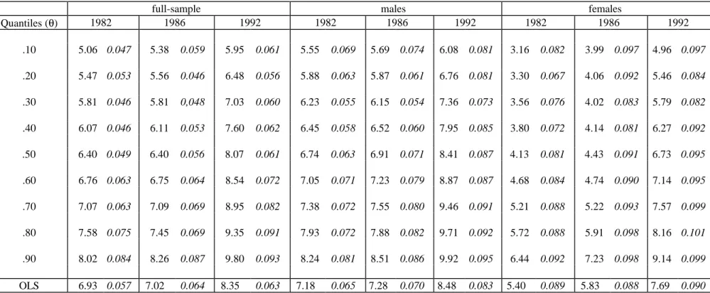
The estimation results are in Tables 5 to 7 in the appendix. All coefficients are significantly different from zero. The QR estimates are also plotted in Figures 5 and 6. The objective of Figure 6 is to compare the returns within a given year. The return to a year of education required and the return to a year of education above the job requirement increase as we move up in the conditional wage distribution. Also, the penalty to year of education below that meant for the job tends to increase at higher quantiles but at much slower pace. This asymmetry is very clear in the picture.

--- insert Figure 5 and Figure 6 about here

---A year of education above that intended for the job receives positive return, although smaller than the return to a year of required education. This is verified across the whole distribution and for the mean (i.e. OLS) regression as well. The percentage points difference in these returns is very equal across all quantiles of the wage distribution (the lines are very parallel). Since both tend to increase with the quantile numbers, the relative difference between them is reduced as one moves up on the distribution. For instance, for men the return to a year of education above the job requirement amounts to 46% of that to a year of required education at θ=0.10 and to 64% at θ=0.90, in 1982. A similar pattern can be found for other years and for women too.

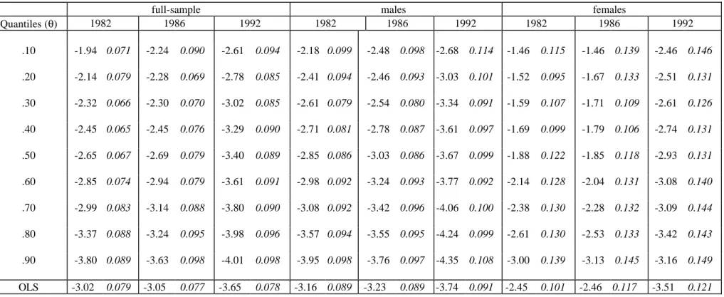
A year of education below the job requirement is penalised in the labour market. Most interesting, the penalty (return) to a year of education below and the rate of return to a year of education above that required for the job diverge as one moves up on the conditional distribution. There is no perceptible difference (in absolute value) between them at low quantiles. As we move up, the return to a year of education above that required for the job becomes progressively larger than that penalty. Analysing “on average” (OLS) misses this peculiar feature.

Now, let’s consider the evolution over time. Figure 6 indicates that the period 1982-86 was characterised by a great stability at all parts of the distribution. The results point to an upward shift in the returns to required education across almost all quantiles from 1986 to 1992. The only apparent exception is for men at θ=0.10. Furthermore, the shift was much more pronounced for women than for men. An upward shift is also visible in returns to a year of education exceeding the job requirement, but mainly for women (and, in this case, more apparent at upper quantiles). For women, the penalty to a year of education below that required for the job increased substantially at all quantiles but one. The exception is at θ=0.90. The figures also show an upward shift for men above θ=0.10 and below θ=0.90.

Let’s summarise the results by quantile for the ORU specification. Again returns to education are higher at higher quantiles. However, for years of education required in the job the differences by quantile are somewhat smaller than we found before: at the 0.90 quantile they are about half to two-thirds higher than at the 0.10 quantile. For years of education above the job requirement we find the almost familiar ratio of double returns at the to compared to the bottom. For years of education below the job requirement, we find a higher penalty at higher quantiles, but the ratio between top and bottom is smaller than 2.

7 Returns to education and changes in wage inequality

Overall wage inequality expanded in Portugal over the 1980s. Changes in the wage structure along two primary dimensions played a major role in this process. First, there was an increase in between-group wage inequality mainly driven by rising returns to education. Second, there was an increase in within-group wage inequality (see details on these developments in Vieira, forthcoming). The returns to education likely played also a role to increase the latter type of inequality.

--- insert Table 8 about here

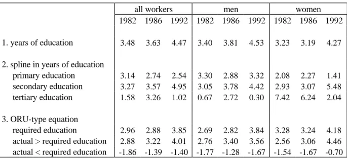
---Differences in log wages between relevant conditional quantiles can be used as measures of within-group wage inequality, see Buchinsky 1994. Using the quantile regressions estimated coefficients we can obtain the marginal effect education upon those measures, see Machado and Mata, 1997. These are obtained by simply computing the differences in the quantile regression coefficients at the relevant quantiles. Results for the two extreme deciles are in Table 8. As we can see, education has a positive effect on within-group wage dispersion. If we give an extra year of education to seemingly equal workers their wages will become more dispersed. Moreover, this marginal effect upon dispersion expanded from 1982 to 1992, except for tertiary education. This is an interesting finding and calls for further research.

8 Conclusions and remarks

This paper was an attempt to provide a comprehensive picture of the returns to education in Portugal and their evolution over the 1980s and early 1990s. For this purpose, we considered alternative specifications of the wage function. Moreover, we used two estimation methods.

The main conclusions can be summarised as follows:

1. There is much heterogeneity in the returns to education. First, returns vary across different margins (i.e. levels) of the schooling distribution. They tend to be higher at higher levels of the schooling distribution. Second, they are lower for females than for males. Third, the effect of a year of education varies according to the allocation in the labour market. Years of education above the job requirement yield a positive return though lower than the return to years of required education. Years of education below that intended for the job are penalised. This fits in with most of the international evidence on the subject.

2. The effect of education on wages is not equal across the conditional wage distribution. Returns are higher for individuals with higher positions in the conditional distribution, with minor exceptions for tertiary education. Apparently the labour force is not reasonably

described by a constant (average) effect of education on wages. Typically, the returns to an extra year of education at the 0.90 quantile are double that at the 0.10 quantile.

3. The returns to education were very stable during the 1982-86 period, but increased substantially from 1986 to 1992. This is valid across the whole wage distribution, although minor exceptions exist. Furthermore, this expansion occurred for men and women but was more pronounced in the latter group. In this catching up process, we must highlight changes occurring in the return to tertiary education for women. In particular, sharp increases took place at the lower part of the conditional wage distribution.

It seems also worthwhile to speculate on the fundamental causes behind the rise of the returns to education. Such an expansion in the price of education occurred along with a shift in the supply of labour towards more-educated workers. In a simple supply-demand setting, observed changes in the price of education require the demand for educated labour to outstrip the rise in supply. In other words, the process is apparently demand-driven.

Skill-biased technological change seems to be the chief explanation for a shift in the demand towards educated labour. This is primary based on the fact that the shift in the use of more-educated labour is due to changes taking place within industries (consistent with technological change) rather than to a reallocation of employment between industries towards sectors requiring high-educated labour (e.g., due to changes in international trade or de-industrialisation), see Vieira et al (1997). Indeed, after 1986 the employment composition shifted towards sectors that traditionally require low-educated rather than high-educated labour such as retail, restaurants and hotels (tourism), construction, textiles, and social services, so this cannot explain the facts. The relevance of forces operating within industries naturally reflects a process of modernisation and may not be independent of joining EU in 1986. First, structural funds from the EU in combination with specific financial aids to industrial investment for modernisation of the productive structure have contributed to the introduction of new technologies. Second, the liberalisation of trade with more developed countries producing capital goods likely encouraged the importation of technology requiring skilled labour.

The increase in the difference of the price of education between the highest and the lowest deciles of the conditional wage distribution has a less clear cut. One way to pursue is to assume that higher returns for workers at higher quantiles likely reflect a complementarity between education and unobserved variables (e.g. ability) to generate wages. Moreover, this complementarity may have strengthened over time (and contributed to expand inequality). We must stress, however, that the development was quite different for tertiary education. Such a divergence between the highest and the other levels of education is naturally an important route for further research.

REFERENCES:

Alba-Ramirez, A. (1993) “Mismatch in the Spanish Labor Market”, Journal of Human Resources, 28, 259-278.

Amstrong, R.; Frome, E. and Kung, D. (1979) “Algorithm 79-01: a revised simplex algorithm for the absolute curve fitting problem”, in Communications in Statistics, Simulation, and Computation B8(2). New York: Marcel Dekker.

Berman, E.; Bound, J. and Griliches, Zvi (1994) “Changes in the Demand for Skilled Labour Within US Manufacturing: evidence from the annual survey of manufacturing”, Quarterly Journal of Economics, 119, 367-397.

Buchinsky, M. (1995) “Quantile Regression, Box-Cox Transformation Model, and the U.S. Wage Structure, 1963-1987”, Journal of Econometrics, 65, 109-154.

Buchinsky, M. (1994) “Changes in the U.S. Wage Structure 1963-1987: application of quantile regression”, Econometrica, 62, 405-458.

Card, D. (1994) “Earnings, Schooling and Ability Revisited”, Working Paper No. 4832, Cambridge, Mass: National Bureau of Economic Research.

Cardoso, A. R. (1997) Earnings Inequality in Portugal: the relevance and the dynamics of employer behaviour, Ph.D. Thesis, Florence: European University Institute.

Chamberlain, G. (1994) “Quantile Regression, Censoring and the Structure of Wages”, in C. Sims and J.J. Laffort (eds.) Proceedings of the Sixth World Congress of the Econometrics Society, Barcelona, Spain. New York: Cambridge University Press, 171-209.

Coelho, H. M.; Soares, L. M. and Feliz, M. I. (1982) Os Níveis de Qualificação na Contratação Colectiva. Sua Aplicação a Algumas Empresas Públicas do Sector dos Transportes e Comunicações. Lisboa: Ministério do Trabalho.

Courakis, A. (1991) “Labour Skills and Human Capital in the Explanation of Trade Patterns”, Oxford Economic Papers, 43, 443-462.

Duncan, G. and Hoffman, S. (1981) “The Incidence and Wage Effects of Overeducation”, Economics of Education Review, 1, 75-86.

Fitzenberger, B. and Kurz, C. (1997) “New Insights on Earnings Trends across Skill Groups and Industries in Germany”, Diskussionspapiers 38, Center for International Labor Economics, Universität Konstanz.

Hartog, J. (1997) “On Returns to Education: wandering along the hills of ORU land”, paper prepared for the keynote speech at the Conference of the Applied Econometrics Association, Maastricht May 15-16.

Hartog, J. (1986) “Allocation and the Earnings Function”, Empirical Economics, 11, 97-110. Hartog, J. (1981) Personal Income Distribution: a multicapability theory, Boston: Martinus

Nijhoff.

Hartog, J. and Oosterbeek, H. (1988) “Education, Allocation and Earnings in the Netherlands: Overeducation?”, Economics of Education Review, 7, 185-194.

Hartog, J. and Tsang, M. (1987) “Estimating, Testing and Applying a Comparative Advantage Earnings Function for the U.S. 1969-1973-1977”, Research Memorandum 8709, Department of Economics, Universiteit van Amsterdam.

Koenker, R. and Basset, G. (1982) “Robust Tests for Heteroscedasticity Based on Regression Quantiles”, Econometrica, 50, 43-61.

Machado, J. A. and Mata, J. (1997) “Earning Functions in Portugal 1982-1994: Evidence from Quantile Regressions”, paper presented at the workshop The Portuguese Labour Market in International Perspective, Lisbon, July 18-19.

Manski, C. (1988) Analog Estimation Methods in Econometrics, London: Chapman & Hall. Mata, J. and Machado, J. (1995) “Firm start-up size: A conditional quantile approach”

European Economic Review, 40, 1305-23.

MESS-DE [Ministério do Emprego e Segurança Social - Departamento de Estatística] (1994) Demografia das Empresas: 1982-1992, Lisboa: MESS-DE.

Mincer, J. (1974) Schooling, Experience and Earnings, New York: National Bureau of Economic Research.

Psacharopoulos, G. (1985) “Returns to Education: a further international update and implications”, Journal of Human Resources, 20, 583-604.

Psacharopoulos, G. (1994) “Returns to Investment in Education: a global update”, World Development, 22, 1325-1343.

Sattinger, M. (1980) Capital and the Distribution of Labor Earnings, Amsterdam: North-Holland.

Sicherman, N. (1991) “Overeducation in the Labor Market”, Journal of Labor Economics, 9, 101-122.

Tinbergen, J. (1956) “On the Theory of Income Distribution”, Weltwirtschaftliches Archiv, 77, 156-173.

Vieira, J. (forthcoming) The Evolution of Wage Structures in Portugal 1982-1992, Tinbergen Institute, forthcoming Ph.D. Thesis.

Vieira, J. Hartog, J. and Pereira, P. (1997) “A Look at Changes in the Portuguese Wage Structure and Job Level Allocation during the 1980s and Early 1990s”, Discussion paper TI 97-008/3, Amsterdam: Tinbergen Institute.

Willis, R. J. (1986) “Wage Determinants: a survey and reinterpretation of human capital wage functions”, in O. Ashenfelter and R. Layard (eds.) Handbook of Labor Economics, Amsterdam: North Holland, 525-602.

Wood, A. (1994) North-South Trade, Employment and Inequality: Changing Fortunes in a Skill Driven World, Oxford: Clarendon Press.

Appendix: Estimation results

Table 1: Rates of return to education (%)

full-sample males females

Quantiles (θ) 1982 1986 1992 1982 1986 1992 1982 1986 1992 .10 3.12 0.068 3.40 0.060 3.55 0.064 3.50 0.072 3.66 0.074 3.69 0.092 1.91 0.073 2.59 0.082 2.99 0.095 .20 3.59 0.051 3.71 0.048 4.38 0.066 3.91 0.061 4.07 0.059 4.70 0.088 2.13 0.068 2.50 0.081 3.50 0.078 .30 3.99 0.052 4.17 0.048 4.96 0.060 4.33 0.077 4.60 0.057 5.45 0.077 2.34 0.062 2.50 0.081 3.88 0.077 .40 4.38 0.059 4.44 0.054 5.53 0.065 4.81 0.078 5.04 0.065 6.00 0.080 2.45 0.062 2.69 0.066 4.32 0.085 .50 4.81 0.071 4.84 0.054 6.08 0.063 5.21 0.087 5.41 0.072 6.59 0.083 2.90 0.066 2.92 0.074 4.75 0.084 .60 5.19 0.067 5.26 0.059 6.57 0.062 5.68 0.081 5.94 0.076 7.07 0.083 3.31 0.065 3.26 0.078 5.09 0.082 .70 5.57 0.069 5.63 0.070 6.95 0.071 5.96 0.079 6.25 0.075 7.50 0.085 3.80 0.068 3.72 0.076 5.63 0.082 .80 5.98 0.079 6.09 0.071 7.46 0.074 6.34 0.081 6.69 0.082 7.88 0.087 4.28 0.071 4.47 0.080 6.18 0.086 .90 6.60 0.092 7.03 0.086 8.02 0.091 6.90 0.088 7.47 0.082 8.22 0.090 5.14 0078 5.78 0.088 7.26 0.092 OLS 5.25 0.053 5.46 0.055 6.38 0.067 5.54 0.063 5.84 0.066 6.56 0.085 3.80 0.091 4.10 0.091 5.71 0.109

Table 2: Rates of return to education, spline estimation (%) [Primary Education]

full-sample males females

Quantiles (θ) 1982 1986 1992 1982 1986 1992 1982 1986 1992 .10 2.08 0.093 2.37 0.099 2.55 0.112 2.56 0.101 2.65 0.118 2.63 0.120 0.91 0.108 1.41 0.128 2.17 0.115 .20 2.65 0.089 2.69 0.093 2.89 0.119 3.22 0.101 3.05 0.127 2.97 0.136 1.13 0.106 1.58 0.127 2.24 0.136 .30 3.04 0.088 2.97 0.087 3.30 0.115 3.53 0.106 3.34 0.121 3.56 0.112 1.20 0.091 1.71 0.110 2.39 0.124 .40 3.29 0.086 3.18 0.092 3.61 0.118 3.77 0.110 3.60 0.124 4.01 0.122 1.55 0.107 1.65 0.106 2.64 0.116 .50 3.52 0.086 3.47 0.101 3.83 0.125 3.99 0.112 3.92 0.128 4.32 0.131 1.88 0.114 1.85 0.111 2.82 0.123 .60 3.78 0.085 3.66 0.098 4.07 0.123 4.21 0.115 4.21 0.131 4.64 0.129 2.13 0.123 2.02 0.133 2.67 0.126 .70 4.07 0.086 3.96 0.100 4.36 0.126 4.57 0.115 4.50 0.132 4.91 0.134 2.37 0.126 2.32 0.129 2.83 0.131 .80 4.47 0.089 4.31 0.108 4.68 0.129 4.95 0.121 4.99 0.132 5.49 0.134 2.76 0.132 2.84 0.136 3.04 0.141 .90 5.22 0.090 5.11 0.110 5.09 0.129 5.86 0.134 5.53 0.135 5.95 0.138 2.99 0.133 3.68 0.139 3.58 0.144 OLS 3.86 0.097 3.88 0.106 4.07 0.132 4.22 0.120 4.25 0.137 4.40 0.148 2.22 0.151 2.50 0.159 3.17 0.151

Table 3: Rates of return to education, spline estimation (%) [Secondary Education]

full-sample males females

Quantiles (θ) 1982 1986 1992 1982 1986 1992 1982 1986 1992 .10 3.75 0.089 3.80 0.105 3.45 0.110 3.87 0.104 3.91 0.128 3.35 0.132 3.01 0.125 3.30 0.132 3.02 0.127 .20 3.91 0.086 3.98 0.086 4.22 0.097 3.85 0.103 4.07 0.111 4.51 0.126 3.15 0.111 2.99 0.131 3.58 0.135 .30 4.14 0.085 4.32 0.086 4.80 0.092 3.98 0.112 4.52 0.106 5.14 0.127 3.29 0.093 2.82 0.121 4.01 0.130 .40 4.44 0.083 4.52 0.093 5.33 0.093 4.27 0.105 4.83 0.124 5.52 0.129 3.25 0.114 3.09 0.106 4.41 0.137 .50 4.94 0.087 4.90 0.091 5.83 0.092 4.76 0.116 5.24 0.111 5.99 0.129 3.50 0.113 3.33 0.110 5.04 0.133 .60 5.44 0.088 5.31 0.096 6.46 0.098 5.38 0.117 5.73 0.114 6.64 0.128 3.98 0.119 3.66 0.122 5.24 0.138 .70 5.83 0.087 5.73 0.097 6.95 0.099 5.88 0.125 6.17 0.116 7.13 0.130 4.54 0.129 4.16 0.130 6.15 0.141 .80 6.21 0.089 6.36 0.097 7.64 0.100 6.33 0.134 6.71 0.129 7.71 0.131 4.94 0.121 4.89 0.130 6.95 0.139 .90 7.02 0.091 7.37 0.099 8.40 0.102 6.92 0.134 7.69 0.133 7.77 0.132 5.94 0.142 6.37 0.139 8.50 0.143 OLS 5.34 0.094 5.47 0.094 6.01 0.111 5.31 0.115 5.65 0.119 5.92 0.146 4.47 0.150 4.39 0.146 5.57 0.169

Table 4: Rates of return to education, spline estimation (%) [Tertiary Education]

full-sample males females

Quantiles (θ) 1982 1986 1992 1982 1986 1992 1982 1986 1992 .10 8.49 0.192 8.37 0.230 11.85 0.230 9.64 0.230 8.95 0.246 12.67 0.256 3.89 0.231 6.39 0.262 11.48 0.291 .20 10.13 0.200 9.93 0.201 13.31 0.194 11.50 0.238 10.93 0.238 13.95 0.256 6.32 0.299 8.64 0.255 12.98 0.275 .30 10.78 0.201 11.00 0.188 13.65 0.183 12.04 0.258 11.80 0.226 14.46 0.249 7.39 0.246 9.73 0.267 12.70 0.267 .40 10.72 0.194 11.57 0.211 13.77 0.186 12.32 0.237 12.28 0.263 14.49 0.277 8.25 0.265 11.02 0.243 13.32 0.282 .50 10.90 0.200 11.57 0.212 13.87 0.213 12.25 0.248 12.09 0.232 14.41 0.265 8.50 0.291 11.23 0.264 13.74 0.268 .60 10.96 0.231 11.47 0.244 13.65 0.235 12.23 0.262 11.68 0.234 14.15 0.256 8.94 0.292 10.90 0.298 13.45 0.280 .70 11.28 0.239 11.28 0.241 13.66 0.245 11.93 0.265 11.81 0.260 13.97 0.274 10.54 0.290 11.83 0.302 13.81 0.289 .80 10.63 0.250 11.56 0.280 13.27 0.282 11.30 0.265 11.85 0.267 13.35 0.280 10.01 0.287 12.15 0.312 14.31 0.307 .90 10.07 0.263 11.63 0.289 12.87 0.291 10.31 0.284 11.67 0.279 12.97 0.291 11.31 0.292 12.63 0.316 13.52 0.319 OLS 10.14 0.216 10.39 0.210 12.82 0.219 10.99 0.256 10.78 0.248 13.2 0.278 7.98 0.325 10.15 0.311 12.64 0.349

Table 5: Rates of return to required education (%)

full-sample males females

Quantiles (θ) 1982 1986 1992 1982 1986 1992 1982 1986 1992 .10 5.06 0.047 5.38 0.059 5.95 0.061 5.55 0.069 5.69 0.074 6.08 0.081 3.16 0.082 3.99 0.097 4.96 0.097 .20 5.47 0.053 5.56 0.046 6.48 0.056 5.88 0.063 5.87 0.061 6.76 0.081 3.30 0.067 4.06 0.092 5.46 0.084 .30 5.81 0.046 5.81 0,048 7.03 0.060 6.23 0.055 6.15 0.054 7.36 0.073 3.56 0.076 4.02 0.083 5.79 0.082 .40 6.07 0.046 6.11 0.053 7.60 0.062 6.45 0.058 6.52 0.060 7.95 0.085 3.80 0.072 4.14 0.081 6.27 0.092 .50 6.40 0.049 6.40 0.056 8.07 0.061 6.74 0.063 6.91 0.071 8.41 0.087 4.13 0.081 4.43 0.091 6.73 0.095 .60 6.76 0.063 6.75 0.064 8.54 0.072 7.05 0.071 7.23 0.079 8.87 0.087 4.68 0.084 4.74 0.090 7.14 0.095 .70 7.07 0.063 7.09 0.069 8.95 0.082 7.38 0.072 7.55 0.080 9.46 0.091 5.21 0.088 5.22 0.093 7.57 0.099 .80 7.58 0.075 7.45 0.069 9.35 0.091 7.93 0.072 7.88 0.082 9.71 0.092 5.72 0.088 5.91 0.098 8.16 0.101 .90 8.02 0.084 8.26 0.087 9.80 0.093 8.24 0.081 8.51 0.086 9.92 0.095 6.44 0.092 7.23 0.098 9.14 0.099 OLS 6.93 0.057 7.02 0.064 8.35 0.063 7.18 0.065 7.28 0.070 8.48 0.083 5.40 0.089 5.83 0.088 7.69 0.090

Table 6: Rates of return to a year of education above the job requirement (%)

full-sample males females

Quantiles (θ) 1982 1986 1992 1982 1986 1992 1982 1986 1992 .10 2.35 0.074 2.55 0.082 2.50 0.091 2.54 0.091 2.55 0.099 2.14 0.104 1.85 0.098 2.14 0.100 2.57 0.105 .20 2.59 0.081 2.71 0.069 2.97 0.079 2.63 0.090 2.62 0.098 2.72 0.103 1.95 0.086 2.22 0.102 3.02 0.104 .30 2.86 0.069 2.91 0.069 3.55 0.083 2.80 0.088 2.82 0.085 3.17 0.104 2.17 0.096 2.13 0.083 3.41 0.099 .40 3.13 0.068 3.22 0.074 4.03 0.084 2.94 0.090 3.17 0.091 3.60 0.098 2.37 0.088 2.21 0.081 3.80 0.098 .50 3.53 0.070 3.51 0.074 4.60 0.080 3.22 0.095 3.53 0.096 4.04 0.097 2.74 0.097 2.65 0.091 4.24 0.100 .60 4.00 0.078 3.87 0.079 5.08 0.091 3.58 0.095 3.95 0.093 4.66 0.991 3.23 0.097 2.90 0.102 4.68 0.101 .70 4.43 0.082 4.39 0.089 5.55 0.091 4.16 0.094 4.48 0.098 5.38 0.101 3.70 0.099 3.32 0.097 5.19 0.105 .80 4.90 0.082 4.90 0.088 6.04 0.097 4.69 0.098 4.99 0.097 5.75 0.100 3.91 0.098 4.03 0.098 5.99 0.105 .90 5.23 0.088 5.77 0.091 6.51 0.098 5.30 0.098 5.95 0.099 5.70 0.103 4.41 0.100 5.20 0.104 7.03 0.104 OLS 3.92 0.083 4.07 0.089 4.53 0.092 3.88 0.092 4.14 0.093 4.10 0.099 3.10 0.097 3.33 0.098 4.67 0.100

Table 7: Rates of return to a year of education below the job requirement (%)

full-sample males females

Quantiles (θ) 1982 1986 1992 1982 1986 1992 1982 1986 1992 .10 -1.94 0.071 -2.24 0.090 -2.61 0.094 -2.18 0.099 -2.48 0.098 -2.68 0.114 -1.46 0.115 -1.46 0.139 -2.46 0.146 .20 -2.14 0.079 -2.28 0.069 -2.78 0.085 -2.41 0.094 -2.46 0.093 -3.03 0.101 -1.52 0.095 -1.67 0.133 -2.51 0.131 .30 -2.32 0.066 -2.30 0.070 -3.02 0.085 -2.61 0.079 -2.54 0.080 -3.34 0.091 -1.59 0.107 -1.71 0.109 -2.61 0.126 .40 -2.45 0.065 -2.45 0.076 -3.29 0.090 -2.71 0.081 -2.78 0.087 -3.61 0.097 -1.69 0.099 -1.79 0.106 -2.74 0.131 .50 -2.65 0.067 -2.69 0.079 -3.40 0.089 -2.85 0.086 -3.03 0.086 -3.67 0.099 -1.88 0.122 -1.85 0.118 -2.93 0.131 .60 -2.85 0.074 -2.94 0.079 -3.61 0.091 -2.98 0.092 -3.24 0.093 -3.77 0.092 -2.14 0.128 -2.04 0.131 -3.08 0.140 .70 -2.99 0.083 -3.14 0.088 -3.80 0.090 -3.08 0.092 -3.42 0.096 -4.06 0.100 -2.38 0.130 -2.28 0.132 -3.09 0.144 .80 -3.37 0.088 -3.24 0.095 -3.98 0.096 -3.57 0.094 -3.55 0.095 -4.24 0.099 -2.61 0.130 -2.53 0.133 -3.42 0.143 .90 -3.80 0.089 -3.63 0.098 -4.01 0.098 -3.95 0.098 -3.76 0.097 -4.35 0.108 -3.00 0.139 -3.13 0.145 -3.16 0.149 OLS -3.02 0.079 -3.05 0.077 -3.65 0.078 -3.16 0.089 -3.23 0.089 -3.74 0.091 -2.45 0.101 -2.46 0.117 -3.51 0.121

Table 8: The impact of education upon within-group wage inequality

all workers men women

1982 1986 1992 1982 1986 1992 1982 1986 1992

1. years of education 3.48 3.63 4.47 3.40 3.81 4.53 3.23 3.19 4.27

2. spline in years of education

primary education 3.14 2.74 2.54 3.30 2.88 3.32 2.08 2.27 1.41

secondary education 3.27 3.57 4.95 3.05 3.78 4.42 2.93 3.07 5.48

tertiary education 1.58 3.26 1.02 0.67 2.72 0.30 7.42 6.24 2.04

3. ORU-type equation

required education 2.96 2.88 3.85 2.69 2.82 3.84 3.28 3.24 4.18

actual > required education 2.88 3.22 4.01 2.76 3.40 3.56 2.56 3.06 4.46

actual < required education -1.86 -1.39 -1.40 -1.77 -1.28 -1.67 -1.54 -1.67 -0.70

Figure 1: International comparisons of educational attainment in 1991

A - Population 25-64 years aged by levels of education

0 10 20 30 40 50 60 70 80 90 100 Austria

Belgium _Denmark Finland France _Germany Ireland

Italy Netherlands Portugal Sweden Spain U.K. Average Percentage

Lower Secondary or Less Upper Secondary Tertiary Education

B - Population with at least upper secondary education by age groups

0 10 20 30 40 50 60 70 80 90 Austria

Belgium _Denmark Finland France _Germany Ireland

Italy Netherlands Portugal Sweden Spain U.K. Average Percentage 25-34-yr-old 35-44-yr-old 45-54-yr-old 55-64-yr-old

Source: OECD (1993), Education at a Glance. The figures in panel A are for the highest level of education completed. Tertiary education includes non-university and university education. The average corresponds to the unweighted mean of all the countries included in the picture.

Figure 2: Quantile Rates of Return to Education full-sample 2.2 3.2 4.2 5.2 6.2 7.2 8.2 .10 .20 .30 .40 .50 .60 .70 .80 .90 quantiles return men 2.2 3.2 4.2 5.2 6.2 7.2 8.2 .10 .20 .30 .40 .50 .60 .70 .80 .90 quantiles return women 0.8 1.8 2.8 3.8 4.8 5.8 6.8 7.8 .10 .20 .30 .40 .50 .60 .70 .80 .90 quantiles return

Figure 3: Quantile rates of return to education within various levels of education: comparison within a given year full-sample (1982) 0 2 4 6 8 10 12 14 16 0.1 0.2 0.3 0.4 0.5 0.6 0.7 0.8 0.9 return men (1982) 0 2 4 6 8 10 12 14 16 0.1 0.2 0.3 0.4 0.5 0.6 0.7 0.8 0.9 return women (1982) 0 2 4 6 8 10 12 14 16 0.1 0.2 0.3 0.4 0.5 0.6 0.7 0.8 0.9 return full-sample (1986) 0 2 4 6 8 10 12 14 16 0.1 0.2 0.3 0.4 0.5 0.6 0.7 0.8 0.9 return men (1986) 0 2 4 6 8 10 12 14 16 0.1 0.2 0.3 0.4 0.5 0.6 0.7 0.8 0.9 return women (1986) 0 2 4 6 8 10 12 14 16 0.1 0.2 0.3 0.4 0.5 0.6 0.7 0.8 0.9 return full-sample (1992) 0 2 4 6 8 10 12 14 16 0.1 0.2 0.3 0.4 0.5 0.6 0.7 0.8 0.9 return men (1992) 0 2 4 6 8 10 12 14 16 0.1 0.2 0.3 0.4 0.5 0.6 0.7 0.8 0.9 return women (1992) 0 2 4 6 8 10 12 14 16 0.1 0.2 0.3 0.4 0.5 0.6 0.7 0.8 0.9 return

Figure 4: Quantile rates of return to education within various levels of education: comparison over time full-sample (primary) 0 1 2 3 4 5 6 0.1 0.2 0.3 0.4 0.5 0.6 0.7 0.8 0.9 return full-sample (secondary) 0 2 4 6 8 10 0.1 0.2 0.3 0.4 0.5 0.6 0.7 0.8 0.9 return full-sample (tertiary) 0 2 4 6 8 10 12 14 16 0.1 0.2 0.3 0.4 0.5 0.6 0.7 0.8 0.9 return men (secondary) 0 2 4 6 8 10 0.1 0.2 0.3 0.4 0.5 0.6 0.7 0.8 0.9 return men (primary) 0 2 4 6 0.1 0.2 0.3 0.4 0.5 0.6 0.7 0.8 0.9 return men (tertiary) 0 2 4 6 8 10 12 14 16 0.1 0.2 0.3 0.4 0.5 0.6 0.7 0.8 0.9 return women (primary) 0 1 2 3 4 5 6 0.1 0.2 0.3 0.4 0.5 0.6 0.7 0.8 0.9 return women (secondary) 0 2 4 6 8 10 0.1 0.2 0.3 0.4 0.5 0.6 0.7 0.8 0.9 return women (tertiary) 0 2 4 6 8 10 12 14 16 0.1 0.2 0.3 0.4 0.5 0.6 0.7 0.8 0.9 return

Figure 5: Quantile rates of return to a year of required education, to a year of education above the job requirement, and to a year of education below the job requirement: comparison within a given year

full-sample (1982) 0 2 4 6 8 10 0.1 0.2 0.3 0.4 0.5 0.6 0.7 0.8 0.9 return men (1982) 0 2 4 6 8 10 0.1 0.2 0.3 0.4 0.5 0.6 0.7 0.8 0.9 return women (1982) 0 2 4 6 8 10 0.1 0.2 0.3 0.4 0.5 0.6 0.7 0.8 0.9 return full-sample (1986) 0 2 4 6 8 10 0.1 0.2 0.3 0.4 0.5 0.6 0.7 0.8 0.9 return men (1986) 0 2 4 6 8 10 0.1 0.2 0.3 0.4 0.5 0.6 0.7 0.8 0.9 return women (1986) 0 2 4 6 8 10 0.1 0.2 0.3 0.4 0.5 0.6 0.7 0.8 0.9 return full-sample (1992) 0 2 4 6 8 10 0.1 0.2 0.3 0.4 0.5 0.6 0.7 0.8 0.9 return men (1992) 0 2 4 6 8 10 0.1 0.2 0.3 0.4 0.5 0.6 0.7 0.8 0.9 return women (1992) 0 2 4 6 8 10 0.1 0.2 0.3 0.4 0.5 0.6 0.7 0.8 0.9 return

Figure 6: Quantile rates of return to a year of required education, to a year of education above the job requirement, and to a year of education below the job requirement: comparison over time

full-sample (required education)

0 2 4 6 8 10 0.1 0.2 0.3 0.4 0.5 0.6 0.7 0.8 0.9 return

full-sample (actual > required education)

0 1 2 3 4 5 6 7 0.1 0.2 0.3 0.4 0.5 0.6 0.7 0.8 0.9 return

full-sample (actual < required education)

0 1 2 3 4 5 0.1 0.2 0.3 0.4 0.5 0.6 0.7 0.8 0.9 return

men (required education)

0 2 4 6 8 10 0.1 0.2 0.3 0.4 0.5 0.6 0.7 0.8 0.9 return

men (actual > required education)

0 1 2 3 4 5 6 7 0.1 0.2 0.3 0.4 0.5 0.6 0.7 0.8 0.9 return

men (actual < required education)

0 1 2 3 4 5 0.1 0.2 0.3 0.4 0.5 0.6 0.7 0.8 0.9 return

women (required education)

0 2 4 6 8 10 0.1 0.2 0.3 0.4 0.5 0.6 0.7 0.8 0.9 return

women (actual > required education)

0 1 2 3 4 5 6 7 0.1 0.2 0.3 0.4 0.5 0.6 0.7 0.8 0.9 return

women (actual < required education)

0 1 2 3 4 5 0.1 0.2 0.3 0.4 0.5 0.6 0.7 0.8 0.9 return