Source localization with vector sensor array during the makai experiment

SOURCE LOCALIZATION WITH VECTOR SENSOR ARRAY

DURING THE MAKAI EXPERIMENT

Paulo Santosa, Paulo Felisbertoa, Paul Hurskyb

a

Institute for Systems and Robotics, University of Algarve, Campus de Gambelas 8005-139, Faro, Portugal.

b

HLS Research Inc., 12730 High Bluff Drive, San Diego, California 92130.

Paulo Jorge Maia dos Santos, Escola Superior de Tecnologia, Universidade do Algarve, Campus da Penha, 8005-139 Faro, Portugal, Fax Nº +351 289 888 405, [email protected].

Abstract: Vector sensors measure both the acoustic pressure and the three components of

particle velocity. Because of this, a vector sensor array (VSA) has the advantage of being able to provide substantially higher directivity with a much smaller aperture than an array of traditional scalar (pressure only) hydrophones. Although several, most of them theoretic, works were published from early nineties, only in the last years due to improvements and availability of vector sensor technology, the interest on field experiments with VSA increased in the scientific community. During the Makai Experiment, that took place off the coast of Kauai I., Hawaii, in September 2005, real data were collected with a 4 element vertical VSA. These data will be discussed in the present paper. The acoustic signals were emitted from a near source (low frequency ship noise) and two high frequency controlled acoustic sources located within a range of 2km from the VSA. The advantages of the VSA over traditional scalar hydrophone arrays in source localization will be addressed using conventional beamforming.

1. INTRODUCTION

The localization of acoustic sources is usually performed with traditional scalar (pressure only) hydrophones. However, recent studies suggest that vector sensors (3 orthogonal collocated particle velocity sensors and one omnidirectional pressure sensor) could improve source localization and provide information in both vertical and azimuthal directions. Vector sensors can be configured into an array of elements, vector sensor array (VSA), where each element measures acoustic pressure and the three components of particle velocity. The main advantage of the VSA is that it captures more acoustic information; hence it provides substantially higher directivity with a much smaller aperture than an array of traditional scalar hydrophones [1].

During the Makai Experiment, that took place off the coast of Kauai I., Hawaii, in September 2005, signals emitted by two high frequency controlled sound sources were collected with a 4 element vertical VSA. We will discuss source localization using a VSA and the advantages these new sensors provide over conventional pressures-only arrays (PA). As a first step toward beamforming distant sources with a vertical VSA, we have oriented our VSA x and y-axis particle velocity sensors with respect to the low frequency signature of our own ship and its known heading.

2. BEAMFORMING WITH A VSA

To resolve source localization with the VSA, the plane wave beamformer is applied and the individual sensor outputs are delayed, weighted and summed in a conventional manner. A single vector sensor has 4 measured quantities, the scalar pressure and the three components of particle velocity,v=[p,v_x,v_y,v_z], that are combined using a weighting vector.

Several approaches to beamforming were presented in [2], but here a weighting vector, w, that uses direction cosines as weights for the velocity components and a unit weight for pressure, has been chosen. Thus, for the i-th element, the weight is given by:

[

]

θ

φ

θ

φ

φ

where i=1,…,N, N is the number of elements in VSA, k_S

r

is the wave number vector corresponding to the chosen steered, or look direction,

(

θ

φ

)

The array elements are equally spaced and located along the z-axis, with the first one in origin of the Cartesian coordinates system, Fig. 1, thusrr =

[

]

For a VSA with N elements, the weighting vector W is of dimension 4N×1 and is defined as: ]. ,.., , [ ) , ( _{S S} w₁ w₂ w_N W

θ

φ

The general expression for the beamformer in direction (

θ

φ

), , ( ) , ( ) , ( _{S S} W _{S S} R WT _{S S} B

θ

φ

θ

φ

θ

φ

where R is 4N×4N correlation matrix.

The azimuth and the elevation of the plane wave impinging on the array are estimated by finding the values(

θ

φ

3. SIMULATION RESULTS

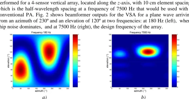
In order to check the VSA beampattern dependency on frequency a few simulations were performed for a 4-sensor vertical array, located along the z-axis, with 10 cm element spacing, which is the half-wavelength spacing at a frequency of 7500 Hz that would be used with a conventional PA. Fig. 2 shows beamformer outputs for the VSA for a plane wave arriving from an azimuth of 230º and an elevation of 120º at two frequencies: at 180 Hz (left), where ship noise dominates, and at 7500 Hz (right), the design frequency of the array.

a) b)

Fig. 2: Ambiguity surface for a plane wave with an azimuth of 230º and an elevation of 120º at: a) 180 Hz and b) 7500 Hz.

The beamformer outputs in Fig. 2 show that the VSA can resolve both vertical and azimuthal directions, which is an advantage over the PA. As in a PA, when the signal frequency is not too far below the design frequency, (as in Fig. 2 b)), the ambiguity surface has a maximum directivity and the sidelobes are negligible. At low frequencies, the mainlobe is larger and directional ambiguity increases (as shown in Fig. 2 a). For frequencies above the design frequency of the array, spatial aliasing occurs (not shown).

4. REAL DATA RESULTS

The data analysed here was acquired by a 4 element vertical VSA, with 10 cm spacing between each element and deployed to 80m depth, during a period of 2 hours on September 20, 2005. The z-axis on VSA was vertically oriented with respect to the bottom. The

orientation of x and y-axis were unknown. The VSA was tied to a vertical cable, with a 100-150 kg weight at the bottom, to ensure that the array stayed as close to vertical as possible.

First, beamforming outputs for low frequency ship noise are presented. Beamforming the signature generated by the research vessel Kilo Moana was a first step to find the orientation of the VSA.

Next, beamforming results are presented to resolve the directions of arrival from high frequency multitones (emitted by two acoustic sources, testbed sources TB1 and TB2, both located at approximately 2 km from the VSA). These two sources were moored near the seafloor at depths of 201 and 98 m, respectively.

A – Beamforming of Ship Noise

As explained above, the VSA was deployed fairly close to the stern of Kilo Moana, with the ship’s engine directly above the array.

a) b)

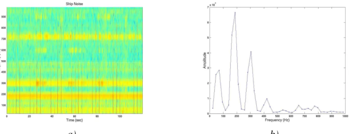
Fig. 3: Noise generated by R/V Kilo Moana on hydrophone at 79.6m depth during the period of acquisition: a) spectrogram and b) power spectrum (1s averaging time).

Observing the data collected by the VSA, at low frequencies, the spectral characteristics of signal are fairly stable over the time. Two dominant frequencies, 180 Hz and 300 Hz, were observed (as shown in Fig. 3). These are assumed to be part of the ship signature and can be used to find the orientation of the VSA about the z-axis.

The correlation matrix of equation (3) is estimated for each frequency using: , 1 1       ⋅ =

∑

where K is the number of snapshots (in this case K=45 corresponding to 1s of data) and the vector Vk represents the FFT bin at the frequency of interest at the k-th snapshot (containing

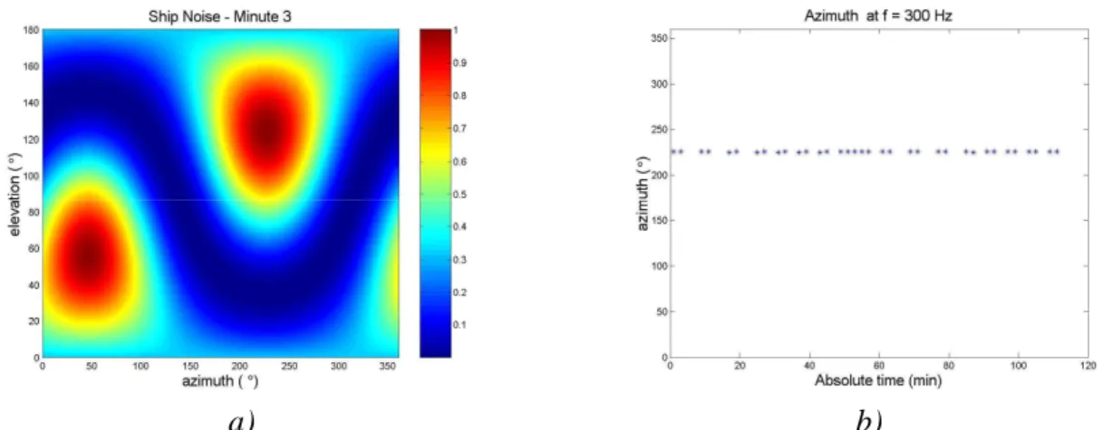
16 VSA channels, 4 measured quantities from each of the four vector sensor elements). Fig. 4 a) shows the results that were obtained when equations (3) and (4) were applied to the real data as a single time epoch. The ambiguity surface using real data is remarkably consistent with the simulations, with the peak at an azimuth of 226º and an elevation of 125º. Fig 4 b) shows that the estimated azimuths do not vary over the processing interval.

Heading data from the ship’s instruments shows that the Kilo Moana was heading in a 50º direction with respect to North, with a maximum displacement of 5º in either direction. Thus one can conclude that the x-axis components of the VSA were oriented approximately to the South and the y-axis components to the West.

a) b)

Fig. 4: Real data beamforming results: a) ambiguity surface for the frequency 300 Hz, at minute 3 and b) estimates of azimuth during period of acquisition.

B – Testbeds Source Localization

In this section source localization results for the testbeds are shown using the orientations of x and y-axis VSA components, estimated in the previous section from the ship signature.

The signals emitted by the two testbeds (TB1 and TB2) were in the 8 - 14 kHz band. The testbed sources periodically transmitted a 2 minute block of of known waveform. Of the various waveforms, beamforming was performed for 8 tones at various frequencies in the 8 - 14 kHz band. The two testbeds each had a distinct set of tones, as well as an 8250 Hz tone that was common to both.

a) b) c)

Fig. 5: Real data beamforming results for frequency 8250 Hz: a) ambiguity surface at minute 1 for TB1; b) ambiguity surface at minute 3 for TB2 and c) estimates of the azimuth during period of

acquisition, for TB1(*) and TB2(^).

The ambiguity surfaces for the multitones received on VSA from TB1 and TB2 are similar to those obtained in simulations, (section 3). Since frequencies of all tones are above 7500 Hz, the design frequency of the array, there is some spatial aliasing and ambiguities in the directions of arrival are observed.

The 8250 Hz tone is the closest to the design frequency of the array, so the beamformer outputs in Fig. 5 exhibit less directional ambiguity. For other frequencies (not shown), the amplitude of sidelobes increases and, for example, the peak output occurs at 333º instead of the true azimuth of 153º.

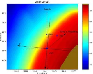
The relative angle between the estimated azimuths of sources TB1 and TB2 shown in Fig. 5 c) does not vary. The fluctuations of the azimuth observed during this interval may be due to ship heading displacements or to rotation of the VSA about the z-axis. However, the estimated azimuths for both sources verify that the source localization is consistent with the known Makai Experiment geometry, shown in Fig. 6.

Fig. 6: Makai experiment geometry with x and y axis orientation.

5. CONCLUSION

The present work showed that a VSA with as few as four elements and a small aperture nevertheless can be used to resolve the directions of arrival of sound sources, not only at frequencies close to the design frequency of the array, but also at frequencies well below this frequency. This improved directivity over a wide range of frequencies made it possible to find the orientation of the x and y-axis particle velocity components of the VSA using the low frequency ship signature. This would have been difficult with a conventional pressures-only array.

The estimated relative angle between two moored sources and the ship, using a simple conventional beamformer at frequencies close to the design frequency of the array, is in close agreement with the experiment geometry. At the same time, ship displacements and the rotation of the array about the z-axis caused the estimates of absolute azimuth to be biased.

The improved spatial filtering capabilities of the VSA, when compared with traditional pressures-only sensor arrays, provide a clear advantage in source localization and related problems, as has been shown in this work and by other authors. It is also likely that these new sensors can open new possibilities for other type of problems, like tomography.

6. ACKNOWLEDGEMENTS

The authors would like to thank Michael Porter, chief scientist for the Makai Exeriment, Bruce Abraham at Applied Physical Sciences for providing assistance with the data acquisition, the SPAWAR Systems Center in San Diego for providing the towed source, and the team at HLS Research for their help with the data used in this analysis. The authors also thank Jerry Tarasek at Naval Surface Weapons Center for the use of the vector sensor array used in this work.

REFERENCES

[1] Arye Nehorai and Eytan Paldi, Acoustic Vector-Sensor Array Processing, IEEE

Transactions on Signal Processing, 42 (9), pp. 2481-2491, September 1994.

[2] Benjamin A. Cray and Albert H. Nuttall, Directivity factors for linear arrays of velocity sensors, JASA, 110 (1), pp. 324-331, July 2001.

[3] Michael Porter et al., The Makai Experiment: High-frequency acoustics, In 8thECUA,