Credit rationing and monetary transmission : evidence for Portugal

Esruoos DE EcoNOMJA, VOL. XIX, N.0 _{1, INVERNO 1999}

CREDIT RATIONING AND MONETARY TRANSMISSION:

EVIDENCE FOR PORTUGAL

Antonio Afonso (*)

Miguel St. Aubyn (**)

1 - Introduction

The purpose of this paper is to evaluate the existence of credit rationing and its relevance to monetary transmission in Portugal during the period from January 1990 to November 1997. Using monthly data we performed two types of tests: stickiness and causality tests. The paper is organised as follows: sec-tion two sets the theoretical and empirical background of credit rasec-tioning and its relevance to the monetary transmission mechanism; the stickiness tests are the object of section three; section four deals with the causality tests and section five is a conclusion.

2 - Credit rationing and monetary transmission

We define «credit rationing» as a situation where demand for loans exce-eds supply at the prevailing interest rate. The price of the loan (the interest rate) does not fully adjust so that demand is not completely satisfied. The rationing of demand may be achieved in two ways: either borrowers do not receive the full amount of credit they have applied for (the so called «type I rationing») or some of the borrowers are simply turned down («type II rationing>>)

(1 ).

In a seminal paper, Stiglitz and Weiss (1981) argue that credit rationing may occur because of asymmetric information in credit markets. Banks (the lenders) have little information on the default risks of the applicants. They have therefore an incentive in not raising interest rates when demand exceeds sup-ply. An adverse selection effect would occur following an interest rate increase that would drive way the less risky applicants. Moreover, an incentive effect would operate because borrowers would be tempted by riskier undertakings. In the end, an interest rate rise would not maximise bank profits as the number of defaults would increase.

(*) lnstituto Superior de Economia e Gestao; lnstituto de Gestao do Credito Publico. (**) lnstituto Superior de Economia e Gestao.

(1) This distinction was due to Keeton (1979) and is widely used in the credit rationing lite-rature. Swank (1996) and Escaria (1997) provide surveys on the theory of credit rationing.

ESTUDOS DE EcoNOMIA, VOL. XIX, N.O 1, fNVERNO 1999

Some authors have argued that rationing in credit markets could be of minor importance once contractual mechanisms like loan commitments and collateral are considered (2_{). The theoretical literature is therefore inconclusive and we,} like Berger and Udell (1992), consider that the existence and importance of credit rationing remains an important empirical issue.

The possible existence of credit rationing opens the way to a credit chan-nel in the transmission mechanism of monetary policy. The credit rationing hypo-thesis implies that monetary contraction would most probably lead banks to contract credit independently of the effect on loan demand of_ any increase in interest rates. Therefore, some degree of stickiness in the adjustment of credit rates to changes in money market rates is to be expected it credit rationing is to have any importance. Also, and still under the credit rationing hypothesis, one expects that monetary policy will have a direct effect on credit, independen-tly of the interest rate channel. These two ideas underlie the two tests we des-cribe in this paper.

We have included a brief review on the empirical evidence on credit ratio-ning in a previous paper

(3).

Tests by surveyed authors basically rely on one of two ideas, also· pursued here:

1) It there is credit rationing, credit rates should not tully respond to chan-ges in money rates (the so called «stickiness tests»). This is the avenue followed by Slovin and Sushka (1983) and Berger and Udell (1992);

if) It there is no credit rationing, the interest rate channel should prevail over the credit channel in the monetary transmission mechanism. This idea is usually exploited by means of ••causality tests» and followed by King (1986) and Sotianos, Wachtel and Melnik (1990).

Results on the empirical relevance of credit rationing are different tor the same economy (the US) according to period and performed test. Table 1, bor-rowed from Afonso and St. Aubyn (1997) summarises results obtained by the aforementioned authors:

(2) See Besanko and Takor (1987) on collateral and Sofianos, Wachtel and Melnik (1990) on loan commitments.

TABLE 1

Some empirical evidence of credit rationing

-

-Author and date Data frequency Period and country Test performed

Slavin and Sushka (1983) ... Quarterly ... 1952:3 to 1980:4 (USA) ... Commercial loan rates adjust to market rates? .... King {1986) ... Quarterly ... 1955:1 to 1979:3 (USA) ... Loan rates are affected by bank liquidity? .... Loan supply responds to loan rate? ... Sofianos, Wachtel and Melnik Monthly ... July 1973 to June 1987 (USA) Direct causality from monetary policy to loans

(1990). not under commitment?

Direct causality from monetary policy to loans under commitment?

Berger and Udell (1992) ... Quarterly ... 1977:1 to 1988:2 (USA) ... Commercial loan rate is «sticky» with respect to open-market rate?

The commitment proportion of new loans rises when open-market rates are high? - -Evidence Results of credit rationing? Yes No Yes Yes Yes No Yes Yes No Yes Yes Partially No No !h'

~

~ [l1

I

~ -~

;;,

--

;; iii

~

ESTUDOS DE ECDNOMIA, VOL. XIX, ·N.0 _{1, 1NVERND ·.1999}

3 - Interest rate stickiness

The credit rationing .hypothesis, namely as stated by Stiglitz and Weiss (1981), implies that credit rates do not ad}ust fully and/or quickly to changes ln money market rates. If money market condffions worsen, banks will not tend to fully reflect these into higher 1nterest rates for their customers.

In this section Ol;Jr empirical investigation is twofold. First, we test the hypo-thesis that money market rates movements ar€ nne to one reflected in credit market .rates ior private companies, no matter of how long this adjustment takes. Then, and having acc:epted the aforementioned hypothesis, we pursue to

esti-mate the speed of adjustment (4_)..

Our data are monthly from December 1990 to November 1997. The money

market rate is TBA (5). Credit market .rates are the average credit rates offered

by banks to private companies, according to cr-edit .length. Four lengths were

considered: 'loans from 91

to

1'80 ·days, lrom 1-81 days to one year, from 2 to 5

years, and more than 5 years.

For several years, between 1978 up to t990, Portugal displayed several

for-ms of direct monetary control where -quantity and price limits were enforced on the banking system and nn 'the credit market. 'However, shortly after the HOs indirect

monetary control started to be implemented and, in a period of more or less three

years, credit and deposit rates were indeed believed to be the result of market demand and supply.

Figure 1 displays the TBA (6) :and two credit rates to non-financFal prhrate

enterprises after 1990. Visual inspeetion swggests that they are quite related. As one would surely expect, money market rates are always bellow credit rates, and falls in those rates seem to impinge on credit rates. Notice that that there was a clear tendency for a fall in interest -rates as Portuguese inflation felt dra-matically ;im this :period.

(4 ) The empirical work in this section updates early empirical work by the same authors -see Afonso and :St. Aubyn (1997).

(5) Average rate of "Treasury Bills auctions.

(6) A similar relation can also be detected with for instance USBOR6 (Lisbon Interbank Offe-ring Rate for a 6 months term).

Esruoos DE EcoNOMIA, VOL XIX, N.0 _{1, INVERNO 1999}

FIGURE 1

Credit rates versus money market rates

30.---.

. . 25 _{---,---,---.---,---,---,---}I I I I I I • I I I I I I I 1 I • I I I o I I I I I I o

.

'

.

' - · - - - J - - - · - - - ' - - - -J -I I 1 I I 20 _{. .} 10 ···-·----~-·-··-····:···~~ ' '

.

.

.

.

.

.

.

. . . 5 - ... --.-- -:- .. - .. - .. -: ... -.-.---;---- .. -.- -:---~---'-.----. I I o I I I I I I o I I ' I I I I o I I o I o t I I I o I I ~+---r· ----~·---r·----~·---+·---r· ----~ !;!

...

"' "'

...

.., N

....

00 "' .... "'

:::

...

..

"'

9

~ "'

...

..

'9 _~ '9 '9 .c> ~ "" C>

:;:

_~ C> e C> _0: "' "'

...

~ ~ ~ ~ ~ _{"' "'} .., ..!, ..!, r!. r!. ~ c-. c-. c-. c-. c-. c-. c-. c-.

... ...

c-.

...

"' c-. "' "'

...

"'

1-TBA

--91-IBOd -<>-18ld-ly

I

{Augmented) Dickey-Fuller tests indicate that all but one interest rates sidered here are well described as stationary around a time trend. 1n what con-cems TBA, we could not dismiss that it is not stationary. The t-statistic on the coefficient of the relevant variable in level where the dependent variable is its .first difference is displayed in table 2, column 2. Under the null hypothesis of no stationarity this statistic follows a Dickey-Fuller distribution. Five percent critical values for this ·number of observations are -3.47 or - 2.90, with and without trend, respectively.

TABLE 2

Stationarity tests for interest .rates and spreads

TBA ... . 91 to 180 days ... . 181 days to 1 year ... . 2 to 5 years ... . More .than 5 years ... .

(•) Significant at 5 percent or less.

Interest rates (levels) Interest rates Spread (relevant 1 - - - . - - - i ( f i r s t differences) cred~ rate- TBA)

Without trend With 1re~d

-0.50 - 0.42 - 1.02 - 0!65 - 1.41 -2.54 (*)-4.70 (*)- 4,16 (*) - 4:89 (*)- 6 .. 34

Without trend Without ·trend (*)- 6.99 (*)- 13.39 (*)- 14.96

n-

14.96 (*)-14.35 (*)- 4.70 (*)-3.98 (*) - 3.51 (*)-5.70

The same type of tests allowed us to r~ject that the f.irst differences are not stationary (table 2, column 3). According to the results of ADF tests, all in-terest Tates bwt TBA would be classified as stationary around a (downward) time

Esruoos DE EcoNOMIA, VOL. XIX, N.0 _{1, INVERNO 1999}

trend. The time trend reflects the fall in inflation observed in the sample years. As it can not be possible that interest rates will be an ever decreasing time series, it is sensible to expect that the fall in interest rates will stop sooner or later, once inflation stabilises. Therefore, we assume the time trend reflects a small sample bias and classify all rates as 1(1)

C).

The difference between the credit rates and the money market rate is called the spread. We have tested the hypothesis that the four spreads we have (the-re is one sp(the-read for each of the c(the-redit rates) a(the-re 1(0), or stationary. We have done that again using the Dickey-Fuller test for stationarity. It is clear by the results in table 2 that the no stationarity null hypothesis is comfortably rejected, without any time trend. The spread displays a constant mean through time, so that TBA is cointegrated with each of the credit rates, with cointegrating vector (1, - 1). Therefore, we conclude that changes in TBA reflect themselves into

one to one

changes in credit rates.

Having concluded that spreads are stationary, we now turn into the esti-mation of the speed of adjustment of credit rates to changes in· money market rates. We want to answer the following question: How long does the spread take to revert to the mean after a change in TBA? The longer the period the stickier credit rates are, once adjustments in the spread after a change in TBA come through changes in credit rates.

To actually estimate the speed of adjustment we have estimated the follo-wing equation for all but one of the four time series of spreads (8):

where the number of lags is such that residuals show no autocorrelation (9). Equation (1) is equivalent to the following one, where

i

is the credit rate (1°):

Recalling that spread =

i -

TBA, equation (2) is a reparameterisation of equation (1) in the error correction form. Table 3 presents the estimated coeffi-cients of equation (2).

(l) We wish to thank an anonymous referee who called our attention to this point.

(8) A time trend never turned to be significant.

(9) Only one lag was needed when. modelling the 2 to 5 year spread.

Esruoos DE EcoNOMIA, VOL. XIX, N.0 _{1, INVERNO 1999}

TABLE 3

Credit rate specification (t-statistics between parenthesis)

Spread (dependent variable) Constant aTBA asp read (- 1) spread (-1)

91 to 180 days ...•... 0.642 0.181 - 0.219 - 0.187 (1.75) (1.62) (- 2.50) (- 2.20) 181 days to 1 year ... 0.719 0.258 - 0.260 - 0.190 (2.17) (2.13) (- 2.83) (- 2.78) 2 to 5 years ... 1.371 0.198 - - 0.301 (3.40) (1.25) (- 3.85)

More than 5 years ... 1.478 0.097 - 0.190 - 0.462

(3.79) (0.47) (- 1.88) (- 4.32)

The estimated equations allowed us to provide an estimate of the adjust-ment speed. We computed the time adjustadjust-ment of the credit rate after a sustai-ned one point increase in TBA. The adjustment in month 0 is given by the coefficient in DTBA. This coefficient is in all cases smaller than one, an indica-tion that credit rates already adjust a little in the same month TBA changes. Changes in the following months are implied by the autocorrelation structure of the credit rate equation, and are presented in table 4.

TABLE 4

Cumulative adjustment (in basis points) of credit rate after an increase of 100 basis points in TBA

91 to 180 days ... . 181 days to 1 year ... . 2 to 5 years ... . More than 5 years ... .

0 18 ?6 20 10 51 59 44 69 2 53 58 61 72 3 61 66 73 84 4 67 71 81 89

One can infer that following a one point increase in TBA, the average cre-dit rate for lending operations from 91 to 180 days increased by only 67 basis points after four months (or 71 basis points, considering operations between 181 days and 1 year).

We conclude that credit rates do not adjust immediately to changes in money market conditions. There is some degree of stickiness in credit rates, which is not against the credit rationing hypothesis. Nevertheless, as time goes by credit rates do adjust fully to changes in money market rates.

EsTuoos DE EcoNOMIA, VOL. XIX, N.0 _{1, INVERNO 1999}

4 - Causality tests

Another possible method of testing for credit rationing is to evaluate the existence of a direct effect of money on loans. In the absence of credit rati-oning credit should always be on the credit demand schedule, and therefore there should not be any direct influence of a money aggregate. One should only expect to find evidence for the interest rate channel, that is, money would have a direct effect on loan rates and loan rates would also be useful to explain credit. Our objective is therefore to see if there is direct causality from money to credit or, in other words, if the credit rationing channel is operative. Moreover, if credit rationing is not relevant, one would not expect credit to affect economic activity, once interest rates have been taken into account. In other words, empirical evidence favouring a credit channel in the monetary transmission mechanism would add to the conviction that credit rationing is at work.

Using monthly data from January 1990 to October 1997 we proceeded to estimate a multivariate VAR model including four variables: a monetary aggre-gate (M1t consistent with a narrow money supply definition; credit to non-fi-nancial enterprises and private individuals; the loans and advances rate for operations from 91 to 180 days and economic activity proxied by the Industrial Production Index (IPI) (11_).

We have used the logarithms of real money and real credit aggregates, as well as the real loan rate. As one could expect from monthly data of this kind,

re~l money and credit and IPI include a strong seasonal pattern. We have taken

the seasonal differences of these variables. As seasonal differencing was not enough to achieve stationarity, we have taken the first difference of the ensuing series. In practice, this means we have used the monthly changes of year-on-year growth rates for these variables

(1

2_).

The real interest rate was not found to be stationary in levels. The first difference was, so that this variable was considered as a 1(1) variable without any significant seasonal pattern. Consequently, monthly changes were used in

(11 ) We did not use monetary base instead of M1· because there was a significant change in monetary policy during the period under analysis: the reduction of the legal reserve coefficient from 17 per cent to 2 per cent in 1994. This resulted in a substantial one time decline (a 61.2 per cent decrease) of monetary base on November 1994.

(12_{) In previous empirical work, we .have used comparable but seasonally adjusted series.}

Esruoos DE EcDNOMtA, VOL. xtx, N." 1, INVERNO 1999 the VAR. In all cases, stationarity was tested using the Augmented Dickey Ful-ler test. Table 5 summarises our stationarity tests:

TABLE 5

Stationarity tests for money, credit, loan rate and IPI (13)

Level Seasonal difference First difference

of seasonal difference (a)

Real money ... . Real credit ... , ... . IPI ... .

Real loan rate ... . - 1,32 (11)

-1,38 (12) 0,44 (12) - 1,51 (11)

(a) Except for the interest rate, where seasonal differencing was not necessary. ( .. ) Significant at 1 percent or less.

(**) - 10,23 (0) (**) - 7,41 (0) (**) - 6,46 (4) (**) - 11 '1 (0)

The VAR specification is given in equations (3) to (6), with all variables transformed as described above

(1

4_):

5 5 5 5

Mt = constant+ L a.mtMt-i +

L

~mPt-i +

L

y miRt-i +

L

0m~t-i + umt (3)

i= 1

5 5 5 5

Ct= constant+

L

a.ciMt-i+

L

~cPt-i+

L

YciRt-i+

L

oc~t-i+ uct (4)

i= 1

5 5 5 5

R1= constant+

L

a.,iMt-i+

L

~rPt-i+

L

YriRt-i+ _Lo~t-i+ urt (5)

i= 1

5 5 5 5

At= constant+

L

a.atMt-i+

L

~aPt-i+

L

YaiRt-i+

L

0a~t-i+ uat (6) where:

M- real money (M1");

C - real credit (loans and advances),

R -

real loan rate =(1+rate)/(1+p)-1); A - IPI index;

i= 1

13 _{Values within parenthesis denote the number of lags for the dependent variable used in}

the Dickey-Fuller or Augmented Dickey-Fuller tests.

14 _{There was no evidence of cointegration among the 1(1) variables, according to Johansen}

P!Ocedure tests, so we proceded to estimate a VAR using differenced variables without any error-correction terms.

Esruoos DE EcoNOMIA, VOL. XIX, N.0 _{1, INVERNO 1999}

rate - nominal loan rate;

p - year on year inflation rate.

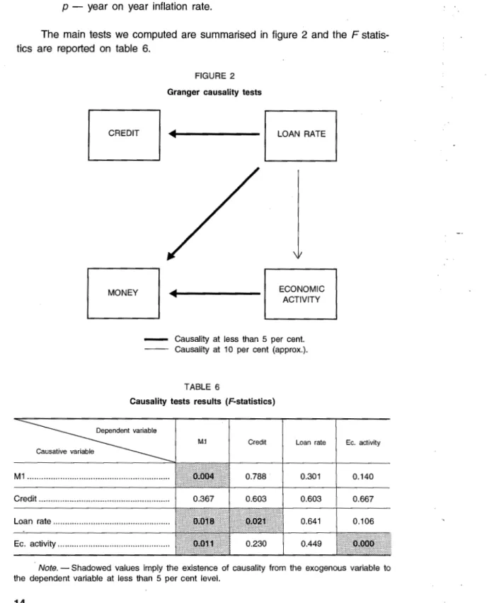
The main tests we computed are summarised in figure 2 and the F statis-tics are reported on table 6.

FIGURE 2 Granger causality tests

~---

I

LOAN RATE

I

ECONOMIC ACTIVITY

Causality at less than 5 per cent. Causality at 10 per cent (approx.).

TABLE 6

Causality tests results (F-statistics)

~ependent

variable

_::sative

v~ia~ ~

M1 Credit Loan rate

M1 ... . 0.788 0.301 Credit ... . 0.367 0.603 0.603 Loan rate ... . 0.641 Ec. activity ... . 0.230 0.449 Ec. activity 0.140 0.667 0.106

Note. - Shadowed values imply the existence of causality from the exogenous variable to the dependent variable at less than 5 per cent level.

£sTUOOS DE £coNOMIA, VOL. XIX, N.0 _{1, fNVERNO 1999}

From the causality tests one can draw some interesting conclusions. The-re is no evidence of cThe-redit rationing in so far as cThe-redit does not seem to be influenced by past values of money and is clearly influenced by the interest rate. This can be interpreted as a sign of credit being on the demand. curve. Econo-mic activity is not Granger-caused by money or credit once the interest rate is taken into account. Apparently, the interest rate channel is at work and not a credit one. The interest rate is not clearly significant in explaining economic activity, though. Nevertheless, its low p-value and the fact that a rise in the interest rate depresses activity, according to the impulse response function dis-cussed below are in accordance with this interpretation.

The fact that the loan rate causes money comes as no surprise. We have seen previously that loan rates are closely related to money rates, which one would expect to relate to a narrow money aggregate. Also, loan rates cause credit, and credit is related to deposits (a part of M1-) by the banks balance sheets. We interpret the remaining causality relationship (from activity to mo-ney) as a standard «demand for money» result.

We have computed impulse response functions from the estimated VAR using the Choleski decomposition method

(1

5). Basically, we had to assume:

1) That innovations to each variable are orthogonal;

i1) A pattern of contemporaneous effects within variables.

Assumption if) is closely related to the usually called «ordering» of the VAR. In the impulse response functions below, we have assumed the following order: activity, credit, loan rate, money. This implies that a variable that is positioned before another is not contemporaneously affected by it. For example, activity was assumed not to be contemporaneously affected by any of the other varia-bles, and money to be contemporaneously affected by all other variables. Al-though there is a degree of arbitrariness in this ordering, it respects the rule that variable X is not contemporaneously affected by Y if Y does not Granger cause X at less than the 5 percent significance level. The shape of the impulse response functions was not very different when other orderings were conside-red.

Impulse response functions concerning the four more significant causal relationships are represented in figures 3 to 6. They trace the response through time of a variable following a standardised change in another variable.

15 _{Charemza and Deadman (1997), Enders (1995) and Sarte (1997) discuss this and other}

EsTUDOS DE ECONOMIA, VOL. XIX, N.0 _{1, INVERNO 1999} 0.006 0.005 0.004 0.003 0.002 0.001 0 -0.001 -0.002 -0.003 0.012 0.01 0.008 0.006 0.004 0.002 0 -0.002 -0.004 -0.006 -0.008 -0.01 0.002 0 -0.002 -0.004 -0.006 -0.008 -0.01 FIGURE 3

Response of credit to loan rate

"

I

/'

I I j

\

!

\

-

~ "'\ a 1'> 1 7 x "" ->a .,., 'J7°

"

'" Aa J:;'l 1:;71

\ -

L

I

I - - - · Months FIGURE 4

Response of money to loan rate

~~;,fy

21

..

25 2" "" "'

...

_{'" "" "'}

I

v

Months FIGURE 5

Response of money to activity

,,

~

_{' ' '}

~ft.

r;·

13 17 21 25 29 33 37 41 45 49 53 57

~

I~

EsTUDOS DE ECONOMIA, VOL. XIX, N. 0 _{1, /NVERNO 1999} FIGURE 6

Response of activity to loan rate

0.004 - - - , 0.002 {\ .A

o

·z ...

-0.002 -lt--6-JV\fl-liAI-1'1-3-'17 21 25 29 33 37 41 45 49 53 57 -0.004 - + 1 - + - - ' - - - ( -0.006 i - t - t - - - ( -0.008 - t - 1 - c l - - - ( -0.01 - t - t - i l - - - j -0.012 - J - f J I - - - t -0.014 - j - - - ( -0.016 _____________________________ ...J Months

As one could expect, an increase in the loan rate depresses credit in the mid-term (figure 3), according to the idea that credit is on the demand schedu-le. The same increase in the loan rate makes money decrease (figure 4). This is probably related to the decrease in credit and therefore in deposits and also to the monetary contraction following a rise in money market interest rates, to which loan rates are closely related. Figure 5 seems to convey the message that money responds positively in the mid-term to activity. Finally, figure 6 impli-es that a rise in the loan rate deprimpli-essimpli-es economic activity (the interimpli-est rate channel), with the caveat that this causal relationship is significant at the 1 0 per-cent level only.

5 - Conclusion

Empirical evidence presented in this paper is not favourable to the existen-ce of credit rationing in Portuguese banking.

Stickiness tests tell us that money market rate changes are transmitted to credit rates changes on a one to one basis. The credit rationing hypothesis would imply that credit rates would observe some degree of independence from mo-ney market rates. This is somehow denied by our stickiness results. It is still the case that credit rates take some time to adjust and that some degree of rationing could still be occurring. Clearly there is scope here for further and more detailed empirical research.

The VAR based tests were not more favourable to rationing in credit ma-rkets. Narrowly defined money does not seem to condition the level of credit, basically determined by the prevailing interest rate and taking economic activity into account. Also, interest rates are more important for economic activity than

Esruoos DE EcoNOMIA, VOL. XIX, N.0 _{1, INVERNO 1999}

credit or money. The authors are aware that these results could arise from misspecification of credit demand or from the choice of variables (namely for money and economic activity). Results should therefore be interpreted with care and more research on the matter is under way.

ANNEX Data sources

Loan rates: loan (to non-financial enterprises and private individuals) rates for various loan lengths, Banco de Portugal.

TBA: average rate of Treasury bills auctions, Banco de Portugal.

Mt·: currency in circulation + demand deposits and other monetary liabilities, Banco de Portugal.

Credit: credit to non-financial enterprises and private individuals, Banco de Portugal. Economic activity: Industrial production index (1990=1 00), mainland, adjusted for working days, Institute Nacional de Estatfstica.

EsTUDOS DE ECONOMIA, VOL. XIX, N.0 _1,

INVERNO 1999 REFERENCES

AFONSO, A., and ST. AUBYN, M. (1997), «Is There Credit Rationing in Portuguese Banking?», working paper N2 _{6/97, Department of Economics, lnstituto Superior de Economia e Gestao,}

Lisboa.

BERGER, A. N., and UDELL, G. F. (1992), «Some Evidence on the Empirical Significance of Credit Rationing», Journal of Political Economy, vol. 100, no. 5, 1047-1077.

BESANKO, D., and TAKOR, A. V. (1987), «Collateral and Rationing: Sorting Equilibria in Monopo-listic and Competitive Credit Markets», International Economic Review, vol. 28, 671-89. CHAREMZA, W., and DEADMAN, D. (1997), New Directions in Econometric Practice, 2nd edition,

Edward Elgar, Cheltenham, United Kingdom.

ENDERS, W. (1995), Applied Econometric Time Series, John Wiley and Sons, New York. ESCARIA, V. (1996), «Uma Analise do Mercado do Credito Admitindo lnforma9ao Assimetrica: 0

Racionamento do Credito e os Mecanismos de Transmissao da Polftica Monetaria», mas-ters dissertation, lnstituto Superior de Economia e Gestao, Lisboa.

KEETON, W. (1979), Equilibrium Credit Rationing, Garland Press, New York.

KING, S. (1986). «Monetary Transmission. Through Bank Loans or Bank Liabilities?» Journal of Money Credit and Banking, vol. 18, no. 3, August, ;290-303.

SARTE, P.-D. (1997). «On the Identification of Structural Vector Autoregressions», Federal Reser-ve Bank of Richmond Economic Quarterly, vol. 83, no. 3, Summer, 45-67.

SLOVIN, M. B., and SUSHKA, M. E. (1983), «A Model of Commercial Loan Rate», The Journal of Finance, vol. xxxv111, no. 5, December, 1538-1596.

SOFIANOS, G., WACHTEL, P., and MELNIK, A. (1990), «Loan Commitments and Monetary Po-licy», Journal of Banking and Finance, 14, October, 677-689.

STIGLITZ, J., and WEISS, A. (1981 ), «Credit Rationing in the Markets with Imperfect Informati-on», The American Economic Review, Vol. 71, N2 _{3, June, 393-410.}

SWANK, J. (1996), «Theories of the Banking Firm: A Review of the Literature», Bulletin of Econo-mic Research, vol. 48, no. 3, 173-207.