1
Improving the effectiveness of predictors in accounting-based models
Duarte Trigueiros
ISTAR-IUL, University Institute of Lisbon [email protected] ABSTRACT
Financial ratios are routinely used as predictors in modelling tasks where accounting information is required. The purpose of this paper is to discuss such use, showing how to improve the effectiveness of ratio-based models. First, the paper exposes the inadequacies of ratios when used as multivariate predictors and then develops a theoretical foundation and methodology to build accounting-based models. From plausible assumptions about the cross-sectional behaviour of accounting data, the paper shows that the effect of size, which ratios remove, can also be removed by modelling algorithms, which facilitates the discovery of meaningful predictors and leads to markedly more effective models. Experiments verify that the new methodology outperforms the conventional methodology, the need to select ratios among many alternatives is avoided, and model construction is less arbitrary. The new methodology can end the uncritical use of modelling remedies currently prevailing and release the full relevance of accounting information when utilised to support investments and other value-bearing decisions.
I. Introduction
Financial institutions, analysts and investors, increasingly rely on multivariate models to assess credit risk, to estimate the likelihood of default, to forecast earnings’ changes, to detect financial misstatement and to carry out other predictive tasks (Ball and Kothari, 1994; Ak et al., 2013). The purpose of this paper is to improve the effectiveness of accounting-based models, something that is probably a minor concern for research-driven modelling but which is vital when the aim is to support actual decisions. In the paper, an improved effectiveness means a higher level of accuracy and explained variability, and the lessening of model-generated biases (Wilcox, 2010).
Published in the Journal of Applied Accounting Research Volume 20, Issue 2 2019, pp. 207-226.
2
Among factors determining model effectiveness, the paper attends to the adequacy of predictors. Accounting-based models use ratios as predictors. Ratios are indeed indispensable in the analysis of financial statements where they bring to light financial features such as Profitability or Solvency while allowing the comparison of varied-size firms. But the fact that ratios are adequate in the context of financial analysis should not exempt them from scrutiny when the purpose is predictive modelling. The specific inadequacies of ratios when used as predictors are the need to find appropriate ratios among many alternatives (Du Jardin, 2009; Xu et al., 2014; Tian et al., 2015) and their erratic, not well-behaved distributions (McLeay, 1986; So, 1987; Lau et al., 1995) that may lead to misrepresentation of essential qualities of the data being modelled (Kotz et al., 2005).
The paper develops a theoretical basis to show that the effect of size, which ratios are able to remove, can also be removed by modelling algorithms. While removing size,
algorithms portray financial features required by the relationship being modelled as though ratios were there, yet avoiding the mentioned inadequacies of ratios. A model-building methodology derived from such theoretical basis is proposed, capable of retaining ratios’ most valuable traits, namely interpretability. Three experiments are performed to compare the new and the conventional methodologies. The experiments verify that the new methodology delivers markedly more accurate, unbiased, and robust prediction.
The findings reported here have the potential to expedite the use of accounting-based models in predictive tasks where to date accuracy is not conclusive enough to support actual decisions. Better investment decisions, for instance, may result from a superior accuracy in predicting earnings’ changes (Ou and Penman, 1989; Holthausen and Larcker, 1992),
takeover targets (Palepu, 1986; Barnes, 1990) and other market-related attributes. Also, in the face of concerns about the declining value-relevance of accounting information (Lev and Gu,
3
2016), the sizeable performance gains now at hand will provide support to the claim that such apparent decline is not intrinsic to accounting information but may result, among other causes, from poorly specified and inadequately constructed models (Clout et al., 2016).
II. Critical review of the use of ratios in accounting-based models
This section exposes ratios’ inadequacies when used as predictors in multivariate models, presenting the case for the proposed methodology and summarising related research. First, the difficulty presented by the need to seek appropriate ratios is delineated. Next, the section calls to mind the cause of ratios´ erratic distributions and the ensuing consequences for modelling. Then, a relevant case of ratio-induced misrepresentation is discussed in relation to current modelling practice. Finally, the propensity of ratios to bias models by selectively generating missing values is examined.
The ratio selection process is unsatisfactory
The selection of multivariate predictors is generally seen as a difficult task and, given the profusion of candidates, such difficulty increases when the predictors are financial ratios. To solve this problem, some authors select predictors on the basis of theory while other authors follow ad-hoc approaches.
When the aim is to test research hypotheses, ratios are pre-selected according to theory. But in Palepu (1986), Beneish (1999), and in other studies where model effectiveness should be a concern, ratios are equally selected on the basis of individual qualities stated by theory. These studies are transposing to the multivariate domain an essentially analytic, univariate routine. The consequence is that the predicting algorithm is limited in its choices, and is unable to use all information available in sets of accounts.
4
Multivariate algorithms are synthesisers. They estimate moments and covariance matrices from multivariate distributions and then they extract from such estimations, and not from any specific ratio, whatever variability is optimal in modelling a relationship. This is why models where effectiveness is important tend to favour the use of ad-hoc approaches to select ratios from a larger set (Altman, 1968; Du Jardin, 2009; Dechow et al., 2011; Xu et al., 2014; Tian et al., 2015), with the view to obtain optimal or nearly optimal prediction. But since the number of ratios that are potentially useful to model a relationship can be very large, some useful ratios may end up not being included in the selection procedure.
Both theory-driven and ad-hoc ratio selection are therefore unsatisfactory for applied modelling. In addition, the task of selecting ratios typically is time-consuming and laden with arbitrary choices. In Altman and Sabato (2007), for instance, this procedure involves 4 steps, including theory- and literature-based ratio gathering, univariate pre-selection, multivariate selection, and backward removal of weak predictors.
The methodology proposed in the paper is able to bypass ratio selection entirely. Variability required to model a relationship is identified as contained in the set of line items directly taken from financial statements, not in ratios. So, rather than being at the inception of the model-building process, ratios follow from the modelled relationship.
Ratio distributions may distort models
The erratic and not well-behaved distributions found in ratios led authors interested in building accounting-based models to propose ad-hoc remedies such as the winsorisation or the pruning of outliers (So, 1987; Lau et al., 1995), the transformation of ratios (Watson, 1990; Altman and Sabato, 2007), or the use of robust estimation (Ohlson, 1980; Zmijewski, 1984). Today, the mentioned ad-hoc remedies continue to be extremely popular (Sun et al.,
5
2014; Ohlson and Kim, 2015; Leone et al., 2017), which suggests that ratio distributions are still treated as mild oddities that need to be addressed somehow.
In fact, distributions of ratios are not odd, and are actually easy to understand. For continuous-valued numbers, randomness is the result of many interacting effects. Effects are aptly known as additive if they add together, or multiplicative if they multiply each other. Additive distributions, such as the Normal distribution, reveal the acting of additive effects, whose likelihood of occurrence is governed by the additive law of probabilities.
Multiplicative distributions, such as the lognormal distribution, likewise reveal effects whose likelihood of occurrence is governed by the multiplicative law of probabilities.
It has long been established that income, wealth, firm size and other economic accruals resulting from the accumulation of random amounts, obey a multiplicative law of probabilities such as the Pareto or the Gibrat laws, and not an additive law such as the Central Limit Theorem (Ijiri and Simon, 1964; Singh and Whittington, 1968). As the statistical behaviour of financial statement numbers approximates other economic accruals, their cross-section distributions obey a multiplicative law of probabilities (McLeay, 1986; Tippett, 1990; Trigueiros, 1995; Falta and Willett, 2011), and ratios formed from them are multiplicative as well (Johnson et al., 1994). Based on this premise, McLeay and Trigueiros (2002) are able to explain the various distributions found in ratios.
Also, ratio distributions are not mild by any measure. In additive data, it is rare to see cases diverging from the mean by more than three standard deviations. The height of human adults, for instance, is limited, as humans are neither taller than mountains nor smaller than mice. Yet, for multiplicative data, such disproportions are, not just possible but likely. In fact, multiplicative distributions display an exponential behaviour, that is, when cases are ranked by magnitude, they raise exponentially. As a consequence, for increasing occurrences of a
6
multiplicative variable, the dispersion of cases increases very rapidly as their density drops abruptly. In the resulting distribution, almost all cases are concentrated in a small interval and a few cases are scattered far away (Johnson et al., 1994).
The term “heteroscedasticity”, that is, an uneven dispersion of cases, does not do justice to the exponential behaviour of ratios. When it is claimed that Least Squares or Maximum Likelihood estimation, being inefficient but not biased regarding
heteroscedasticity, can be used in ratio-based modelling (Ohlson, 1980), it is clear that such claim ignores the multiplicative nature of ratios where extremely influential cases will distort model coefficients directly while the mentioned abrupt drop in the density of cases, which cannot be replicated with any approximation by a Least Squares or Maximum Likelihood fit (Kotz et al., 2005), will lead to models where distributions are misrepresented. It is also clear that the type of extreme observation found in multiplicative data is not necessarily aberrant. Therefore, pruning or winsorisation is, not just counterproductive but it may be a source of bias (Leone et al., 2017).
The new methodology deals adequately with the multiplicative behaviour of line items, dispensing ad-hoc remedies and making modelling less arbitrary.
Ratios may misrepresent class likelihoods in classification tasks
Most accounting-based models are classifiers (Amania and Fadlallab, 2017), and a long lived example (Altman, 1968, 1983) predicts firm failure using a balanced sampling design where classes contain nearly the same number of failed and not failed cases.
Today, balanced sampling is rarely used, admittedly because it leads to biased estimates (Palepu, 1986). Such bias, however, does not alter the position of estimated likelihoods relative to each other so that, when the purpose is to find the cases that are the
7
most and least likely to belong to the class of interest, balanced sampling is not only adequate, but is also the most information-efficient design (Cosslett et al., 1981).
In an attempt to prevent the said bias, class frequencies in model-building datasets are nowadays made to mimic the underlying prevalence, that is, the real-world class likelihoods. If, say, the a priori chances of failure are 6 out of 100, then the model-building dataset must contain 6% of failed firms and 94% of not failed firms.
There are reasons to discourage such practice. First, prevalence is often small, which may impair the generalisation ability of models when there are not sufficient cases belonging to the minority class to represent its distribution adequately (Zmijewski, 1984). This damage is especially visible in tasks such as the prediction of acquisition targets (Palepu, 1986) and the detection of financial misstatement (Beneish, 1999) where both prevalence and predictive power are small. Second, class frequencies in the data available for modelling seldom reflect prevalence and data must be manipulated in one form or another before becoming usable. Inevitably, such manipulation will create new biases. Finally, if no attempt is made to get to grips with the exponential behaviour of ratios, predicted class frequencies will be
misrepresented, being pointless to make model-building classes resemble prevalence. There are procedures available to appropriately account for class imbalances. Besides the option of using estimation methods compatible with balanced sampling (Manski and MacFadden, 1981), it has been demonstrated that, when the modelling algorithm is the Logistic regression, class imbalance affects the intercept coefficient only, so that models can be built from balanced samples and then intercepts can be corrected to take imbalance into account (Xie and Manski, 1989).
The new methodology brings to an end misrepresentation of distributions in
8
data manipulation is not needed. When appropriate, balanced sampling opens the way to the use of matching and other methods able to control for undesirable characteristics of the data.
Ratio-generated missing values may also misrepresent class likelihoods
Most accounting-based empirical research relies on third-party databases of financial
statements. It is increasingly feared that data quality issues may affect research results. Here, Casey et al. (2016) review the literature on financial statements’ database quality. Among other problems, these authors identify the existence of too many missing values.
Besides poor database quality, a source of missing values is the use of ratios, where any one missing component, or a zero-valued denominator, will create a new missing value. Missing values will distort models when the number of cases withdrawn is related to the variable being predicted. For example, firms not paying dividends in the previous period will be removed from earnings-predicting models where a popular predictor is the change in Dividends per Share relative to the previous period.
The paper presents instances of ratio-generated, class-dependent missing values, showing how the new methodology helps reducing the consequent bias.
III. A new model-building methodology
This section develops a theoretical basis from which a new model-building methodology is derived. The underlying premise is that, except in well-known cases, financial ratios can be validly used in the analysis of financial statements. More than one hundred years of scrutiny and intensive use testify in favour of such premise.
Valid use of ratios rests on the assumption that ratios are capable of removing the effect of size, thus making financial features comparable across firms of different sizes. From
9
this, two corollaries follow (McLeay and Trigueiros, 2002). First, a common effect,
accounting for differences in size among sets of accounts, is present in the two components of the ratio and is removed when the ratio is formed. Second, such effect is removed when the two components are multiplicative, that is, when they have distributions where effects multiply each other. Indeed, when a ratio is formed from two numbers having in common the same factor, that factor is offset.
The most general instance of multiplicative behaviour is the lognormal distribution. When lognormality is hypothesised, the two corollaries just mentioned require that the cross-sectional variability of 𝑥 , the ith line item from the jth set of accounts, be described as
𝐿𝑜𝑔 𝑥 𝑚 𝑧 𝜖 (1)
where the logarithm of 𝑥 is explained as an expectation 𝑚 accounting for the overall mean and the deviation from the mean specific to item 𝑖, plus 𝑧 , the size effect specific to set of accounts j, plus size-unrelated residual variability 𝜖 .
Formulation (1) is not intended to minutely portray the cross-sectional behaviour of line items, but to describe 𝑧 , the common effect of size. The 𝜖 are not necessarily
independent and, after size is accounted for, there may remain positive or negative correlations between the residuals of any two line items.
Given two line items, 𝑖 1 and 𝑖 2 and the corresponding 𝑥 and 𝑥 from the same set of accounts, the logarithm of the ratio of 𝑥 to 𝑥 is, according to (1), written
𝐿𝑜𝑔 𝐿𝑜𝑔 𝑥 𝐿𝑜𝑔 𝑥 𝑚 𝑚 𝜖 𝜖 (2)
where, trivially, the effect of size, 𝑧 , is no longer present. The median ratio 𝑒𝑥𝑝 𝑚 𝑚 is a suitable norm against which comparisons can be made, while 𝑒𝑥𝑝 𝜖 𝜖 is the
10
deviation from this norm observed in the ratio. For example, 𝑒𝑥𝑝 𝜖 𝜖 shows whether the Operating Ratio is above or below the norm. Thus 𝜖 𝜖 is, in logarithms, the information conveyed by a ratio about a financial feature.
To the extent that ratios are suitable as analytical tools, premises leading to (1) are more or less verified. If this were not so, then ratios from large firms would behave
differently from ratios from small firms. Profitability, for instance, would not be of any use in cross-sectional analysis.
The case of line items where negative values occur
Formulation (1) cannot explain negative values, such as those found in Net Income. But line items where negative values occur are subtractions of two positive-only items. Consider 𝑥 𝑥 𝑥 where 𝑥 and 𝑥 are positive. For any sign of 𝑥, an algebraic manipulation leads to
𝐿𝑜𝑔 |𝑥 𝑥 | 𝐿𝑜𝑔 𝑥 𝐿𝑜𝑔|1 |. (3)
Since 𝑥 is positive, (1) applies to 𝐿𝑜𝑔 𝑥 . And since, as shown in (2), is
size-independent, 𝑧 is not present in 𝐿𝑜𝑔|1 |. Using the notation adopted in (1), the expected
value of 𝐿𝑜𝑔 |𝑥 𝑥 | is written as 𝑚 , being the result of adding 𝑚 to the expected value of 𝐿𝑜𝑔|1 |. Similarly, residuals are written as 𝜖 . From (3),
𝐿𝑜𝑔 |𝑥| 𝑚 𝑧 𝜖 (4)
for positive- and negative-valued 𝑥. Although 𝑚 and 𝜖 in (4) no longer have the intuitive meaning of 𝑚 and 𝜖 in (1), notably 𝑧 in (4) is exactly the same as in (1). Basically this is the
reason why ratios remove the effect of size, even when one component is negative. Now, if ratios remove size no matter the sign of components, it should be possible to use any item,
11
not just positive-valued items, in modelling tasks requiring the removal of size. When items are transformed so that the effect of size is preserved regardless of sign as in (4), their subtraction will remove size in a way similar to (2), also regardless of sign.
One such size-preserving transformation is 𝐿𝑜𝑔 |𝑥| coupled with a dummy retaining the sign of 𝑥. In classification tasks, dummies may be replaced by a fixed displacement 𝑑 of 𝐿𝑜𝑔 |𝑥| for negative 𝑥 only, where 𝑥 is transformed into 𝐿𝑜𝑔 |𝑥| 𝑑 .
Another transformation worth mentioning at this stage is 𝑠𝑖𝑔𝑛 𝑥 𝐿𝑜𝑔 |𝑥|, known as Log-Modulus (John and Draper, 1980), where negative 𝑥 are transformed into 𝐿𝑜𝑔 |𝑥|. Here, the sign of 𝑥 is preserved but a subtraction of two items will not remove size from negative values. Log-Modulus is an alternative to be considered when the goal is simply to transform multiplicative variables into well-behaved variables and size is not an issue, as in the case of models in which the predicted variable is independent of size.
Within the range 1 𝑥 1, the mentioned transformations are equivocal but monotonic alternative exist. Also, since multiplicative numbers require an accumulation to be formed, zero values should be treated as not multiplicative and kept as zeros.
The role of firm size in the modelling of size-independent relationships Consider the relationship
𝑦 𝑎 𝑏 𝐿𝑜𝑔 𝑥 𝑏 𝐿𝑜𝑔 𝑥 ⋯ (5)
where 𝑥 , 𝑥 … are line items taken from the same set of accounts and 𝑦 is the attribute to be predicted. In the case of a classifier, y is the underlying linear score. Where predictors obey (1), then (5) is
12
where 𝐴 𝑎 𝑏 𝑚 𝑏 𝑚 ⋯ is constant. That is, variability available to model y has a size-independent term 𝑏 𝜖 𝑏 𝜖 ⋯ and a size-related term 𝑏 𝑏 ⋯ 𝑧 .
Consider a size-independent 𝑦. The term 𝑏 𝑏 ⋯ 𝑧 must be zero so as to bar size-related variability from entering the relationship. Coefficients 𝑏 , 𝑏 , … will add to zero. When such size-independent 𝑦 is predicted by just 2 logarithm-transformed items, then (5) is
𝑦 𝑎 𝑏 𝐿𝑜𝑔 𝑥 𝑏 𝐿𝑜𝑔 𝑥 with 𝑏 𝑏 𝑏, that is,
𝑦 𝑎 𝑏 𝐿𝑜𝑔 𝑥 𝐿𝑜𝑔 𝑥 or 𝑦 𝑎 𝑏 𝐿𝑜𝑔 . (7)
Ratio 𝑥 to 𝑥 is formed in response to 𝑦’s size-independence. Suppose, for instance, that the ratio 𝑥 to 𝑥 predicts bankruptcy accurately. When the logarithms of its components are shown to a modelling algorithm, the linear combination explaining bankruptcy optimally is found when 𝑏 𝑏 as in (7) because, at that point, size is removed, the ratio is formed and its predictive power is released. When a size-independent 𝑦 is predicted by 3 line items, then 𝑏 𝑏 𝑏 and (5) now is 𝑦 𝑎 𝑏 𝐿𝑜𝑔 𝑏 𝐿𝑜𝑔 . That is, in response to
size-independence, 2 ratios are formed from 3 line items.
In the general case, size-independent 𝑦 might indeed induce 𝑁 1 ratios from 𝑁 line items, but algorithms are not capable of pairing items two-by-two. Instead, as part of the modelling process, size-related variability will be allotted to a number of predictors in order to offset size-related variability in other predictors. The algorithm will assign the role of ‘ratio denominator’ to some predictors (negative-signed 𝑏 coefficients) and that of ‘ratio numerator’ to others (positive-signed 𝑏 coefficients) so that 𝑏 𝑏 ⋯ 0, the overall effect being the removal of size. The ensuing linear combinations are high-dimensional ratios in logarithmic space. Being size-independent, they are capable of portraying financial
13
are meant to preserve size, items where negative values occur will equally form linear combinations capable of removing size. When, for instance, 𝐿𝑜𝑔 |𝑥| 𝑑 is applied to 𝑥 , 𝑥 … in (5), the term 𝑏 𝑏 ⋯ 𝑧 𝑑 will be formed where 𝑑 is distinct but
constant for positive and negative values. As before, size-independent relationships will
cause 𝑏 𝑏 ⋯ 0.
The conclusion to be drawn at this stage of the paper is that the task of selecting ratios capable of portraying financial features while removing size is not a modelling pre-requisite. In response to size-independence, the algorithm will form optimal high-dimensional ratios from logarithm-transformed items. From two predictors, the algorithm will form one ratio.
The case of size-related relationships
When a size-related 𝑦 is modelled by individual items as in (5), size is not fully offset. The term 𝑏 𝑏 ⋯ 𝑧 in (6) creates dependencies in coefficients and algorithms will face multicollinearity. Models that incorporate financial ratios plus a size proxy as predictors, are immune to this complication because, even when size is present in a relationship, ratios cannot account for it. But then again, ratios are unsuitable for multivariate prediction.
By adding to (5) the condition 𝑏 𝑏 ⋯ 0, size-independent variability will explain the size-independent part of the variability of 𝑦. Such condition holds when, instead of 𝑁 items as in (5), 𝑁 1 pairs subtracted as in (7), that is, 𝐿𝑜𝑔 𝑥 𝐿𝑜𝑔 𝑥 , are used as predictors. Similar to ratios, subtracted pairs are intrinsically size-independent. The spare degree of freedom should be utilised to account for the effect of size.
14 The methodology
Logarithm-transformed line items may be used directly in the modelling of size-independent relationships as in (5). Here, financial features will be formed while the effect of size is offset as though ratios were there. Predictors obeying (1) are well-behaved but models’ coefficients cannot be interpreted, a characteristic which is at variance with analysts’ practice and, unlike in models using ratios, magnitude-related alterations would require the rebuilding of models. Consistent with the previous discussion, the new methodology in now outlined. First, the comprehensive set of 𝑀 logarithm-transformed line items, together with the attribute to be predicted, is shown to the modelling algorithm as in (5). A model is built with the sole purpose of selecting the subset of 𝑁 ≪ 𝑀 line items possessing predictive power. Then, at a second stage, pairs made of the 𝑁 items selected at the first stage are subtracted, forming predictors similar to 𝐿𝑜𝑔 𝑥 𝐿𝑜𝑔 𝑥 in (7). No more than 𝑁 1 pairs should be formed and none of the 𝑁 selected items should be omitted. The algorithm estimates the final model using such pairs as predictors.
By selecting predictors from the comprehensive set of 𝑀 line items and not from the much more numerous and ill-defined set of potentially useful ratios, the new methodology greatly simplifies the predictor-selection process while reducing the chances of overlooking variability possessing predictive power.
In the following, practical suggestions to implement the methodology are offered. 1. Databases of financial statements typically scale all numbers down by one million.
Items must be descaled to avoid falling within the range 1 𝑥 1. For the same reason, pre-existing ratios such as Earnings per Share will also need scaling.
15
2. When items have negative values, 𝐿𝑜𝑔 |𝑥| 𝑑 is suited for classification tasks where 𝑑 should exceed the descaling power, that is, for a 10 descaling, then 𝑑 6. Above such threshold value, the choice of 𝑑 is irrelevant. Dummies, in
turn, are suited for regression tasks.
3. If second-stage accuracy is visibly smaller than first-stage accuracy, the relationship is size-related. A size proxy should be added to the list of second-stage predictors while the first stage of the methodology typically requires trial and error to identify the less significant items.
4. Changes ∆𝑥 and ∆𝑥/𝑥 in relation to the previous period are both transformed into
∆ 𝐿𝑜𝑔 𝑥 𝐿𝑜𝑔 𝑥 𝐿𝑜𝑔 𝑥 (8)
where 𝑡 1 and 𝑡 are subsequent periods. In the case of positive- and negative-signed 𝑥, a sign-preserving transformation is required and ∆ 𝐿𝑜𝑔 𝑥 will be size-related. Contrary to ratios, (8) will not create missing values when 𝑥 0.
IV. Three experiments
This section illustrates the use of the new methodology, comparing conventional models based on ratios with first-stage models based on transformed line items and their subtracted pairs, that is, second stage models. Comparisons cover three well-documented classification tasks illustrating low, median and high levels of difficulty, namely bankruptcy prediction, financial misstatement detection and earnings forecasting. Here, classification tasks are preferred to regression tasks because, in the former, model effectiveness is easier to compare.
The three comparisons are made through a controlled experimental design where, except for the predictor used, all other model characteristics i.e. data utilised to build and test
16
models, class frequencies, modelling algorithm, randomisation, and information made available, are strictly identical for the ratio-based and the newly-developed model.
Experiments contemplate ex-ante and ex-post prediction, independent and size-related relationships, and balanced sampling as well as data not subject to sampling. In ratio-based models, cases are not pruned. At the first stage of the new methodology, line item 𝑥 to be tested for inclusion (i.e. Table 1), is descaled into original values and then,
for 𝑥 1, 𝑥 is transformed into 𝐿𝑜𝑔 𝑥; for 𝑥 0, 𝑥 is not transformed;
for 𝑥 1, 𝑥 is transformed into 𝐿𝑜𝑔| 𝑥| 𝑑 for bankruptcy
prediction, and into 𝐿𝑜𝑔| 𝑥| for earnings forecasting. No negative values occur in the misstatement detection experiment.
The transformation applied in the first stage is used in the calculation of (8) and in the second stage. The Logistic regression is the modelling algorithm used throughout the three experiments and first-stage selection of predictors is performed via standard variable-selection algorithms attached to the Logistic regression. Multicollinearity is checked in first-stage models.
-- Table 1 --
Bankruptcy prediction
The first experiment follows Altman’s (1968, 1983) bankruptcy predicting models. Ohlson (1980), Zmijewski (1984) and Taffler (1982) discuss bankruptcy prediction and offer alternatives to Altman’s models. A review of this research, where high accuracy levels are customary, can be found in Balcaen and Ooghe (2006) and in Sun et al. (2014).
17
The experiment aims, not so much at illustrating the benefits of the new methodology, but at introducing its distinctive characteristics. A total of 2,997 bankruptcy filings are drawn from the UCLA-LoPucki data1 and from other sources. Filings but the first to occur in each
firm, and filings about which financial statements are not available, are discarded. Both ‘Chapter 7’ and ‘Chapter 11’ filings are included.2 Two samples of nearly 900 cases each are
drawn from the remaining filings. The two samples contain firms listed in U. S. exchanges, present in the Compustat file. They span the period 1979-2008. All size categories, computed as the deciles of the logarithm of Assets, and all the 24 Global Industry Classification
Standard (GICS) groups are represented.
To lessen unwanted variability, firms in the two samples are matched with firms not bankrupt. Matching is based on the GICS group, on size decile and on year. One bankrupt case is randomly assigned to its peer and then the peer is made unavailable for matching. One of the datasets is utilised to build the models and the other to measure their effectiveness.
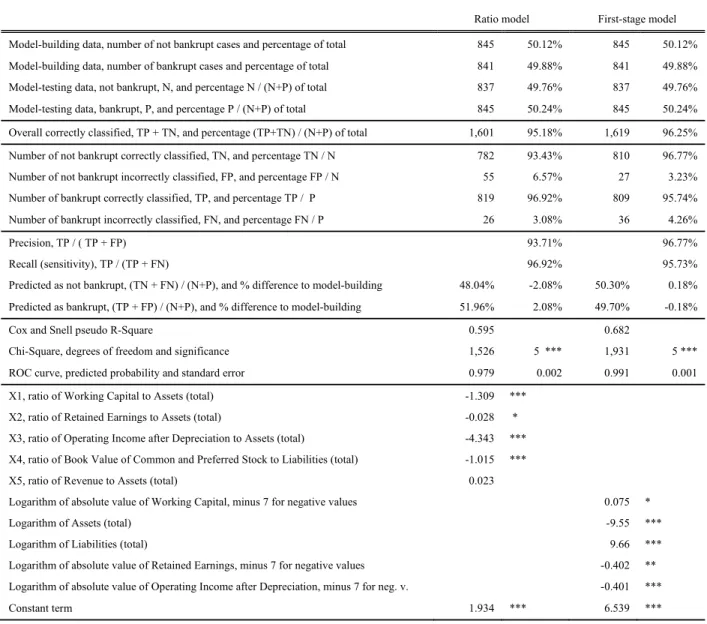
The ratio-based model uses Altman’s (1983) X1 to X5 ratios detailed in Table 2. At the first stage of the new methodology, the algorithm selects 5 predictors from components of the same X1 to X5 ratios. Negative values are transformed into 𝐿𝑜𝑔 |𝑥| 𝑑 , where the chosen 𝑑 7 slightly exceeds the 10 descaling.
Table 2 shows that accuracy is high in both models but ratios fail to use variability available in their components, as Chi-square and R-Square statistics are visibly higher in the first-stage model than in the model based on ratios. Table 2 also compares class frequencies in the model-building dataset with class frequencies predicted by the model.
-- Table 2 --
1http://lopucki.law.ucla.edu/
18
Size-offsetting, mentioned in relation to (5), is visible in first-stage coefficients. Working Capital and Total Liabilities have positive signs and add to 9.74. These are the numerators of internal ‘ratios’. The denominators are Total Assets, Retained Earnings and Operating Income after Depreciation, with negative signs and adding to 10.35.
The 5 predictors selected at the first stage are now paired and the components of each pair are subtracted, forming 4 new predictors to be used at the second stage. Among other possible combinations, the algorithm may estimate the score
0.95 0.13 𝐿𝑜𝑔 𝑊𝐶𝐴𝑃 𝐴𝑇 7.92 𝐿𝑜𝑔 𝐿𝑇 𝐴𝑇 0.47 𝐿𝑜𝑔 𝑅𝐸 𝐿𝑇 0.43 𝐿𝑜𝑔 𝑂𝐼𝐴𝐷𝑃 𝐿𝑇
where abbreviations refer to Table 1 and, in order to emphasise model interpretability, subtractions of two paired items are depicted as “𝐿𝑜𝑔” followed by the fraction sign.
𝐿𝑜𝑔 , for instance, really means 𝐿𝑜𝑔|𝑊𝐶𝐴𝑃| 𝑑 𝐿𝑜𝑔 𝐴𝑇 where 𝑑 is zero
for positive 𝑊𝐶𝐴𝑃 and 7 for negative 𝑊𝐶𝐴𝑃. Zero 𝑊𝐶𝐴𝑃 remain zero.
This model has the same R Square as that at the first stage. Chi-square is 1,912 with 4 degrees of freedom (df). Overall accuracy is 96.2% with 96.9% not bankrupt and 95.6% bankrupt cases correctly classified. Performance is the same for other pairings of the 5 items. Sincesize is not required in this particular case, second-stage performance, based on size-independent predictors, is not smaller than first-stage performance.
Detecting misstated sets of accounts
Sets of accounts are extremely efficient in revealing financial features of firms and this efficiency is the ultimate reason why accounts are so often misstated (Eilifsen and Messier, 2000). Predictive models can help detect misstatement (Beneish, 1999; Dechow et al., 2011; Sun et al., 2014) with an overall accuracy of around 80% for non-homogeneous samples and
19
93% for homogeneous samples (Liou, 2008). In these models, however, the minority class is poorly predicted while the opposite class is predicted very well, which makes them useless.
The second experiment compares the ex-ante effectiveness of a misstatement detection model based on ratios with that of a similar model based on positive-only,
logarithm-transformed line items. Misstated accounts are defined as having been the object of an Accounting and Auditing Enforcement Release resulting from investigations made by the U. S. Securities and Exchange Commission for alleged accounting misconduct.3 Releases are
divided in two sets, one with cases from years 1978 to 1999 and the other with cases from years 2000 to 2008. The 1978-1999 set is utilised in model-building, the 2000-2008 set is utilised to measure the effectiveness of models. The two sets are matched with an equal number of firms which are neither the object of releases throughout the period nor are bankrupt in the release year. Matching is based on the GICS group, size decile and statement year. One misstatement case is randomly assigned to its peer and then the peer is made unavailable for future matching.
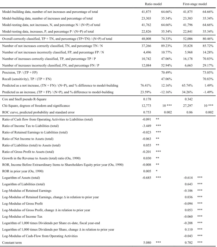
In order to build the ratio-based model, ratios taken from Beneish (1999) and from other studies are shown to the selection algorithm. As detailed in Table 3, 12 ratios are selected, where 5 are from Beneish. Overall accuracy is 74%. False-positives are far more likely than false-negatives and predicted class frequencies diverge widely from frequencies in the model-building dataset.
-- Table 3 --
The dataset utilised to build the ratio model has 358 missing and 781 not missing values. To allow comparison, these 358 cases are taken from the first- and second-stage models, although here the number of missing values is only 18. At the first stage, line items
20
made present to the selection algorithm are components of ratios that entered the ratio-based model, and their changes, computed as in (8). Table 3 shows the selected 7 line items and 2 changes. Overall accuracy is now 84% and predicted class frequencies closely follow frequencies in the model-building dataset. The variability explained is almost twice that of the ratio-based model. It is therefore clear that ratios fail to use much variability available in their components. Again, size offsetting is clearly visible: Cash, Liabilities and Capital, have negative-signed coefficients, magnitudes adding to 15.4. Assets, Receivables, Debt and Revenue, have positive signs, magnitudes adding to 16.2.
From the 7 items selected at the first stage, 5 pairs are formed at the second stage, as nothing is to be gained by adding a sixth pair. ∆ 𝐿𝑜𝑔 𝐿𝑇 is included but the other change also selected, ∆ 𝐿𝑜𝑔 𝐶𝐻𝐸, is non-significant here. From such predictors, the algorithm estimates the score 5.90 3.48 ∆ 𝐿𝑜𝑔 𝐿𝑇 1.87 𝐿𝑜𝑔 𝐶𝐻𝐸 𝑅𝐸𝑉𝑇 9.75 𝐿𝑜𝑔 𝐴𝑇 𝐿𝑇 0.77 𝐿𝑜𝑔 𝐶𝑆𝑇𝐾 𝑅𝐸𝐶𝑇 0.26 𝐿𝑜𝑔𝐶𝑆𝑇𝐾 𝐷𝐿𝑇𝑇 0.51 𝐿𝑜𝑔 𝐶𝑆𝑇𝐾 𝑅𝐸𝑉𝑇
where subtractions of two transformed items are depicted as “𝐿𝑜𝑔” followed by the fraction sign, and “∆” refers to (8).
This second-stage model has the same R Square as that at the first stage. Chi-square is 696 with 6 df. Overall accuracy is 84% with 87% not misstated and 81% misstated cases correctly classified.
Forecasting the direction of earnings’ changes one year ahead
The third experiment is inspired by Ou (1990), who offers evidence on the ability of ratios to forecast the direction of unexpected changes in Earnings per Share one year ahead. Ou and
21
Penman (1989), Holthausen and Larcker (1992) and others, use Ou’s model in the prediction of market returns while Bird et al. (2001) examine the robustness of Ou’s model to different time periods and industries and include a review of published research where the reported predictive gains are poor, by some 6% to 10% at best.
The distinctive features of the experiment are the absence of sampling, the large number of cases (of which predicted classes can be computed) and a size-related relationship. The experiment also highlights biases that ratio-generated, class-dependent missing values create on predicted class frequencies. Amid ratios used by Ou (1990), the percentage change in Inventory to Assets has 20% missing earnings’ decreases while for increases it is 43%. Changes in Dividends per Share relative to the previous year have 29% missing decreases while for increases it is 57%.
When missing values are put aside, some 140,000 cases remain, where nearly 65% are not increases and 35% are increases. From this dataset, two samples with the same size are drawn at random, one for model-building and the other for measuring the effectiveness of models. All ratios in Ou (1990) plus other ratios are tested for inclusion. Ratios formed from Net Income or related items are not excluded from selection. The algorithm selects 9 ratios as detailed in Table 4, of which 3 are from Ou (1990). A size proxy, the logarithm of Assets, is also included in the ratio-based model, bringing the total number of predictors to 10.
When building the model obeying the new methodology, predictors are taken from components of ratios selected by the ratio-based model and their changes computed as in (8). The change in Dividends per Share relative to the previous year fails ratio-selection but, after being transformed as in (8), is selected to enter at the first stage. Negative values are
transformed into 𝐿𝑜𝑔 |𝑥|, which would be an inadequate transformation for size-independent relationships but is not particularly inadequate here. The first stage selects 6
22
transformed line items, plus Dividends per Share, plus 3 changes. Class frequencies, performance, coefficients and significance, are also displayed in Table 4.
-- Table 4 --
Accuracy of the ratio-based model is 74% with 89% not increases and 47% increases correctly classified. Class frequencies observed in the model-building dataset are grossly misrepresented. First-stage accuracy is 80% with no class misrepresentation. The variability explained is twice that obtained in the ratio-based model.
At the second stage, 4 pairs are formed from 5 of the 6 items selected at the first stage. The remaining item, 𝐿𝑜𝑔 𝐴𝑇, takes the role of size proxy and is not paired. The score
0.420 0.108 𝐿𝑜𝑔𝑅𝐸 𝐿𝑇 0.044 𝐿𝑜𝑔 𝑂𝐴𝑁𝐶𝐹 𝐿𝑇 0.061 𝐿𝑜𝑔 𝑇𝑋𝑇 𝐿𝑇 0.095 𝐿𝑜𝑔 𝐺𝑃 𝐿𝑇 0.256 𝐿𝑜𝑔 𝐴𝑇 0.036 ∆ 𝐿𝑜𝑔 𝑅𝐸 0.054 ∆ 𝐿𝑜𝑔 𝐺𝑃 0.107 ∆ 𝐿𝑜𝑔 𝐷𝑉𝑃𝑆 0.205 𝐿𝑜𝑔 𝐷𝑉𝑃𝑆 is estimated, where subtractions of two transformed items are depicted as “𝐿𝑜𝑔” followed by the fraction sign, and “∆” refers to (8). The accuracy, balance and the R Square of this second-stage model are the same as that at the first stage. The Chi-square is 27,143 for 9 df.
Summary and additional evidence
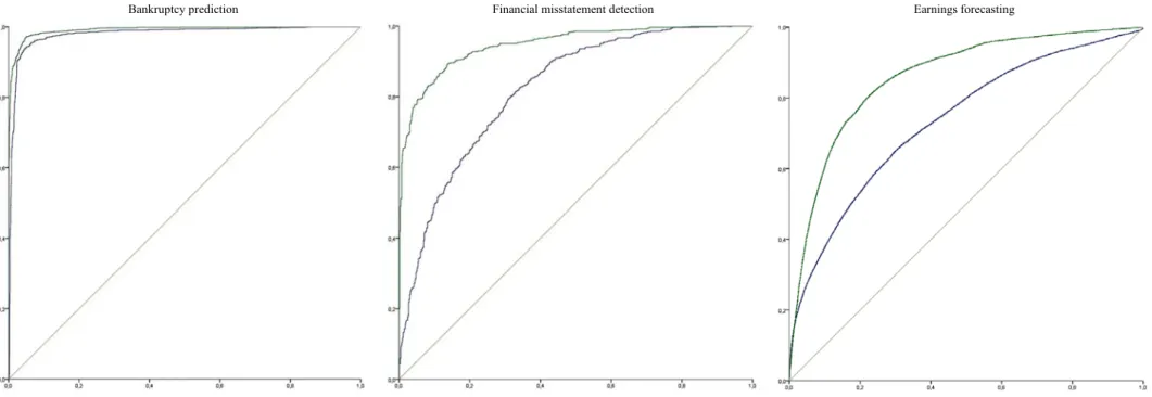
In addition to demonstrating the gains in accuracy that can be obtained with the new methodology, the three experiments show how ratio-based models can grossly misrepresent distributions. In fact, the improvements brought by the new methodology are mainly due to the fact that predicted class frequencies now resemble model-building frequencies. Figure 1 compares ROC curves of ratio-based and second-stage models, where the dominance of the latter and the asymmetry of the former are visible.
23
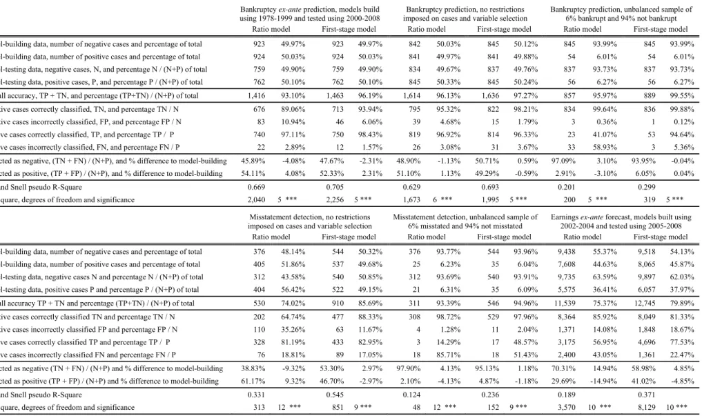
Table 5 tests the robustness of results to the relaxing of restrictions imposed by the experimental design. Sets of predictors are now the best possible sets, and the number of cases available for modelling now depends only on the number of missing values, no longer being constrained to be the same for ratio-based and first-stage models.
-- Table 5 --
Under these new conditions, three types of models are compared:
Ex-ante predictive accuracy is tested using bankruptcy prediction and earnings forecasting.
Two cases of imbalanced samples are examined, where the proportion of the minority class (bankruptcy and misstatement) is 6% of the original number of cases, and the number of cases in the opposite class is unchanged.
The best possible bankruptcy prediction and misstatement detection models are built from balanced sampling designs.
It is verified that ex-ante accuracy is similar to balanced sampling accuracy. For the two imbalanced designs, accuracy deteriorates visibly, with the minority class being ignored. An increase in accuracy is observed in the best possible misstatement detection models.
V. Conclusion
Invariably, ratios are the predictors used in multivariate modelling tasks where accounting information is required. Such use, however, raises difficulties posed by the need to select ratios among many alternatives, by the erratic and not well-behaved distributions of ratios, and by their propensity to misrepresent essential characteristics of the data being modelled. The paper has developed a theoretical basis from which a model-building methodology to bypass the mentioned inadequacies of ratios is derived. Experiments have shown that the new
24
methodology preserves ratios’ meaning while delivering markedly more accurate, unbiased and robust models.
In addition to expanding the use of accounting-based models for tasks that have so far failed to achieve a usable level of accuracy, the reported gains in effectiveness strengthen the conviction that the apparent irrelevance of accounting information may result from the use of poorly specified and inadequately constructed models.
So, before other causes are examined, limitations of accounting-based models should be attributed to the uncritical use of ratios. The multiplicative behaviour of ratios, which aptly leads to size-removal in financial analysis, makes ratios unsuitable for modelling. Ignorance about this incompatibility of ratios, coupled with the use of modelling designs which are incongruous with the objectives pursued when modelling, are the reasons for the limited effectiveness of accounting-based models.
Developments reported in the paper are the consequence of explicitly considering the effect of firm size. When size is modelled as a statistical effect, it is easy to explain why ratios remove size from cross-sections of financial statement numbers, and it is equally easy to show that size can be removed by modelling algorithms.
It is suggested in the paper that models should be built in two stages. First, the reduced set of line items able to explain the relationship optimally is found. At the second stage, adequately transformed ratios are formed from the reduced set. The final model is estimated using the transformed ratios. In addition to gains in effectiveness, modelling becomes less arbitrary because predictors are now selected from a smaller, well-defined list of candidates, and ad-hoc remedies, such as the pruning of extreme cases, are no longer necessary.
25
The methodology is limited in scope, as it aims to improve model accuracy and robustness, and reduce biases, which are minor concerns when the aim is to test research hypotheses. Also, only cross-sectional and size-independent relationships are considered, and accounting identities and other interactions between line items are ignored. The paper is therefore an initial step and the notional approximation from which the new methodology is constructed may at a later stage be refined and adapted to other purposes.
Reference list
Ak, B., Dechow, P., Sun, E. and Wang, A. (2013), "The use of financial ratio models to help investors predict and interpret significant corporate events", Australian Journal of Management, Vol. 38 No. 3 pp. 553-598.
Altman, E. (1968), “Financial ratios, discriminant analysis and the prediction of corporate bankruptcy”, The Journal of Finance, Vol. 23 No. 4 pp. 589-609.
Altman, E. (1983), Corporate Financial Distress: a Complete Guide to Predicting, Avoiding, and Dealing with Bankruptcy, Wiley, New York.
Altman, E. and Sabato, G. (2007), “Modelling credit risk for SMEs: evidence from the U.S. market”, Abacus, Vol. 43 No. 3, pp. 332–357.
Amania, F. and Fadlallab, A. (2017), “Data mining applications in accounting: a review of the literature and organizing framework”, International Journal of Accounting Information Systems, Vol. 24 pp. 32–58.
Balcaen, S. and Ooghe, H. (2006), “35 years of studies on business failure: an overview of the classic statistical methodologies and their related problems”, The British Accounting Review , Vol. 38 No. 1 pp. 63–93.
26
Barnes, P. (1990), “The prediction of takeover targets in the U.K. by means of multiple discriminant analysis”, Journal of Business Finance and Accounting, Vol. 17 No. 1 pp. 73-84.
Beneish, M. (1999), “The detection of earnings manipulation”, Financial Analysts Journal, Vol. 55 No. 5 pp. 24–36.
Bird, R., Gerlach, R. and Hall, A. (2001), “The prediction of earnings movements using accounting data: an update and extension of Ou and Penman”, Journal of Asset Management, Vol. 2 No. 2 pp. 180–195.
Casey, R., Gao, F., Kirschenheiter, M., Li, S. and Pandit, S. (2016), “Do compustat financial statement data articulate?”, Journal of Financial Reporting , Vol. 1 No. 1 pp. 37–59.
Clout, V., Falta, M. and Willett, R. (2016), “Earnings in firm valuation and their value relevance”, Journal of Contemporary Accounting and Economics, Vol. 12 No. 3 pp. 223–240.
Cosslett, S., Manski, C. and McFadden, D. (1981), “Efficient estimation of discrete choice models”, in Structural Analysis of Discrete Data with Econometric Applications, Vol. 3 pp. 51-111, The MIT Press, Cambridge (MA).
Dechow, P., Weili, G., Larson, C. and Sloan, R. (2011), “Predicting material accounting misstatements”, Contemporary Accounting Research , Vol. 28 No. 1 pp. 17–82.
Du Jardin, P. (2009), “Bankruptcy prediction models: how to choose the most relevant variables?”, Bankers, Markets & Investors, Vol. 98 pp. 39–46.
Eilifsen, A. and Messier, W. (2000), “The incidence and detection of misstatement: a review of and integration of archival research”, Journal of Accounting Literature, Vol. 19 pp. 1-43.
Falta, M. and Willett, R. (2011), “Multiplicative regression models of the relationship between accounting numbers and market value”, working paper, available at SSRN.
Holthausen, R. and Larcker, D. (1992), “The prediction of stock returns using financial statement information”, Journal of Accounting and Economics, Vol. 15 No. 2 pp. 373-411.
27
Ijiri, I., and Simon, H. (1964), “Business firm growth and size”, The American Economic
Review, Vol. 54 No. 2 pp. 77–89.
John, J., and Draper, N. (1980), “An alternative family of transformations”, Journal of the Royal
Statistical Society, Series C Vol. 29 No. 2 pp. 190–197.
Johnson N., Kotz, S. and Balakrishnan, N. (1994), “Lognormal distributions”, in Continuous Univariate Distributions, Vol. 1, Wiley, New York.
Kotz, S., Balakrishnan, N. and Johnson, N. (2005), Continuous Multivariate Distributions: Models and Applications, Vol. 1, Wiley, New York.
Lau, H. Lau, A. and Gribbin, D. (1995), “On modelling cross-sectional distributions of financial ratios”, Journal of Business Finance and Accounting, Vol. 22 No. 4 pp 521–549.
Leone, A., Minutti-Meza, M. and Wasley M. (2017), “Influential observations and inference in accounting research”, Simon Business School Working Paper FR 14-06.
Lev B., and Gu, F. (2016), The End of Accounting and the Path Forward for Investors and Managers, Wiley, New York.
Liou, F. (2008), “Fraudulent financial reporting detection and business failure prediction models, a comparison”, Managerial Auditing Journal Vol. 23 No. 7 pp. 650-662.
Manski, C. and MacFadden, D. (1981), Structural analysis of discrete data with econometric
applications. The MIT Press, Cambridge (MA).
McLeay, S. (1986), “The ratio of means, the mean of ratios and other benchmarks”, Finance,
Journal of the French Finance Society, Vol. 7 No. 1 pp. 75-93.
McLeay, S. and Trigueiros, D. (2002), “Proportionate growth and the theoretical foundations of financial ratios.” Abacus, Vol. 38 No. 3 pp. 297–316.
Ohlson, J. (1980), “Financial ratios and the probabilistic prediction of bankruptcy”, Journal of Accounting Research , Vol. 18 No. 1 pp. 512–534.
28
Ohlson, J., and Kim, S. (2015), “Linear valuation without OLS: the Theil-Sen estimation approach”, Review of Accounting Studies, Vol. 20 No. 1 pp. 395-435.
Ou, J., and Penman, S. (1989), “Financial statement analysis and the prediction of stock returns”,
Journal of Accounting and Economics , Vol. 11 No. 4 pp. 295-329.
Ou, J. (1990), “The Information content of non-earnings accounting numbers as earnings predictors”, Journal of Accounting Research, Vol. 28 No. 1 pp. 144–163.
Palepu, K. (1986), “Predicting takeover targets, a methodological and empirical analysis”, Journal of Accounting and Economics , Vol. 8 No. 1 pp. 3-35.
Singh, A. and Whittington, G. (1968), Growth, Profitability and Valuation, Cambridge University Press.
So, J. (1987), “Some empirical evidence on the outliers and the non-Normal distribution of financial ratios”, Journal of Business Finance and Accounting, Vol. 14 No. 4 pp. 483–496.
Sun, J., Li, H., Huang, Q. and He, K. (2014), “Predicting financial distress and corporate failure: a review from the state-of-the-art definitions, modelling, sampling, and featuring approaches”,
Knowledge-Based Systems, Vol. 57 pp. 41-56.
Taffler, R. (1982), “Forecasting company failure in the UK using discriminant analysis and financial ratio data”, Journal of the Royal Statistical Society, Vol. A-145 No. 3 pp. 342-58.
Tian, S., Yu, Y. and Guo, H. (2015), “Variable selection and corporate bankruptcy forecasts”,
Journal of Banking and Finance , Vol. 52-C pp. 89-100.
Tippett, M. (1990), “An induced theory of financial ratios”, Accounting and Business Research, Vol. 21 No. 81 pp. 77-85.
Trigueiros, D. (1995), “Accounting identities and the distribution of ratios”, British Accounting
29
Watson, C. (1990), “Multivariate distributional properties, outliers, and transformation of financial ratios”, The Accounting Review , Vol. 65 No. 3 pp. 682-695.
Wilcox, R. (2010), Fundamentals of Modern Statistical Methods, Springer, New York.
Xu, W., Xiao Z., Dang X., Yang D. and Yang, X. (2014), “Financial ratio selection for business failure prediction using Soft Set theory”, Knowledge-Based Systems , Vol. 63 pp. 59-67.
Xie, Y. and Manski, C. (1989), “The logit model and response-based samples”, Sociological Methods and Research, Vol. 17 No. 3 pp. 283–302.
Zmijewski, M. (1984), “Methodological issues related to the estimation of financial distress prediction models”, Journal of Accounting Research, Vol. 22 pp. 59-82.
Table 1
Line items used in experiments
CHE Cash and Short-Term Investments * RE Retained Earnings * RECT Receivables (total) * SEQ Shareholders' Equity (total)
INVT Inventories (total) REVT Revenue (total) *
ACT Current Assets (total) * XOPR Operating Expense (total) *
WCAP Working Capital * COGS Cost of Goods Sold
PPENT Property Plant and Equipment (total, net) GP Gross Profit (loss) *
INTAN Intangible Assets (total) XSGA Selling, General and Administrative Expenses
AT Assets (total) * DP Depreciation and Amortization (total)
AP Account Payable/Creditors (trade) OIADP Operating Income after Depreciation *
XACC Accrued Expenses XINT Interest and Related Expense
TXP Income Taxes Payable TXT Income Tax (total) *
LCT Current Liabilities (total) * IB Income Before Extraordinary Items
DLTT Long-Term Debt (total) * NI Net Income (loss)
LT Liabilities (total) * OANCF Net Cash Flow from Operating Activities * BKVL Book Value of Common and Preferred Stock CAPX Capital Expenditure
PSTK Preferred Stock EPS Earnings per Share (basic, before extraordinary items) CSTK Common/Ordinary Stock * DVPS Dividends per Share (ex-date, fiscal) *
The table lists the 32 line items plus 2 pre-existing ratios tested for inclusion at the first stage of the new methodology, where both current values and changes (8) in relation to prior year are tested, and also the components of ratios tested for inclusion in ratio-based models. Asterisks show items selected at the first stage by any one of the three experiments. Item values, abbreviations and names are taken from the Compustat file, except BKVL which is computed from other items in the same file.
Table 2 Bankruptcy prediction
Ratio model First-stage model
Model-building data, number of not bankrupt cases and percentage of total 845 50.12% 845 50.12% Model-building data, number of bankrupt cases and percentage of total 841 49.88% 841 49.88% Model-testing data, not bankrupt, N, and percentage N / (N+P) of total 837 49.76% 837 49.76% Model-testing data, bankrupt, P, and percentage P / (N+P) of total 845 50.24% 845 50.24% Overall correctly classified, TP + TN, and percentage (TP+TN) / (N+P) of total 1,601 95.18% 1,619 96.25% Number of not bankrupt correctly classified, TN, and percentage TN / N 782 93.43% 810 96.77% Number of not bankrupt incorrectly classified, FP, and percentage FP / N 55 6.57% 27 3.23% Number of bankrupt correctly classified, TP, and percentage TP / P 819 96.92% 809 95.74% Number of bankrupt incorrectly classified, FN, and percentage FN / P 26 3.08% 36 4.26%
Precision, TP / ( TP + FP) 93.71% 96.77%
Recall (sensitivity), TP / (TP + FN) 96.92% 95.73%
Predicted as not bankrupt, (TN + FN) / (N+P), and % difference to model-building 48.04% -2.08% 50.30% 0.18% Predicted as bankrupt, (TP + FP) / (N+P), and % difference to model-building 51.96% 2.08% 49.70% -0.18%
Cox and Snell pseudo R-Square 0.595 0.682
Chi-Square, degrees of freedom and significance 1,526 5 *** 1,931 5 ***
ROC curve, predicted probability and standard error 0.979 0.002 0.991 0.001
X1, ratio of Working Capital to Assets (total) -1.309 ***
X2, ratio of Retained Earnings to Assets (total) -0.028 *
X3, ratio of Operating Income after Depreciation to Assets (total) -4.343 *** X4, ratio of Book Value of Common and Preferred Stock to Liabilities (total) -1.015 ***
X5, ratio of Revenue to Assets (total) 0.023
Logarithm of absolute value of Working Capital, minus 7 for negative values 0.075 *
Logarithm of Assets (total) -9.55 ***
Logarithm of Liabilities (total) 9.66 ***
Logarithm of absolute value of Retained Earnings, minus 7 for negative values -0.402 ** Logarithm of absolute value of Operating Income after Depreciation, minus 7 for neg. v. -0.401 ***
Constant term 1.934 *** 6.539 ***
Top to bottom: sample size, accuracy, predicted class frequencies and differences in relation to model-building class frequencies, goodness-of-fit statistics, and model coefficients. All line items are descaled by10 before transformed. ‘Logarithm’ refers to base 10 logarithm. All zero values are kept as zero. ‘T’ means correctly classified, ‘F’ means incorrectly classified. Significances are shown as asterisks: ‘***’ is p 0.001, ‘**’ is p 0.01 and ‘*’ is p 0.05.
Table 3
Financial misstatement detection
Ratio model First-stage model
Model-building data (1976-1999), number of not misstated and percentage of total 376 48.20% 376 48.20% Model-building data (1976-1999), number of misstated and percentage of total 405 51.80% 405 51.80% Model-testing data (2000-2008), not misstated, N, and percentage N / (N+P) of total 312 43.57% 312 43.57% Model-testing data (2000-2008), misstated, P, and percentage P / (N+P) of total 404 56.42% 404 56.42% Overall correctly classified, TP + TN, and percentage (TP+TN) / (N+P) of total 530 74.02% 602 84.08% Number of not misstated correctly classified, TN, and percentage TN / N 202 64.74% 272 87.18% Number of not misstated incorrectly classified, FP, and percentage FP / N 110 35.26% 40 12.82% Number of misstated correctly classified, TP, and percentage TP / P 328 81.19% 330 81.68% Number of misstated incorrectly classified, FN, and percentage FN / P 76 18.81% 74 18.32%
Precision, TP / ( TP + FP) 74.89% 89.19%
Recall (sensitivity), TP / (TP + FN) 81.19% 81.68%
Predicted as not misstated, (TN + FN) / (N+P), and % difference to model-building 38.83% -9.37% 48.32% 0.12% Predicted as misstated, (TP + FP) / (N+P), and % difference to model-building 61.17% 9.37% 51.68% -0.12%
Cox and Snell pseudo R-Square 0.335 0.596
Chi-Square, degrees of freedom and significance 312 12 *** 707 9 ***
ROC curve, predicted probability and standard error 0.821 0.011 0.947 0.005
DSRI, Days Sales in Receivables index, see caption 0.178 *
SGI, Sales growth = Revenue / Revenue prior year 0.435 *
DEPI, Depreciation to Property, Plant and Equipment, see caption 0.921 ** SGAI, Sales, General and Administrative Expenses index, see caption 0.439 *
LVGI, Leverage index, see caption 0.737 **
Ratio of Net Income to Revenue 0.120 **
Receivables growth = Receivables / Receivables in prior year -0.062 * Current Ratio = Current Assets (total) / Current liabilities (total) 0.142 *
Ratio of Revenue to Assets (total) 1.140 ***
Ratio of Cash and Short Term Investments to Assets (total) -2.298 ***
Ratio of Inventories to Assets (total) 1.574 *
Ratio of Liabilities (total) to Assets (total) -4.426 ***
Logarithm of Cash and Short-Term Investments -1.733 ***
Logarithm of Cash and Short-Term Investments, change ∆ in relation to prior year 0.481 *
Logarithm of Receivables (total) 0.549 **
Logarithm of Assets (total) 11.31 ***
Logarithm of Long-Term Debt 0.230 ***
Logarithm of Liabilities (total) -11.82 ***
Logarithm of Liabilities (total), change ∆ in relation to prior year 3.760 ***
Logarithm of Common/Ordinary Stock (Capital) -1.80 ***
Logarithm of Revenue (total) 4.186 ***
Constant term -1.118 -15.47 ***
Caption of Table 2 applies here. DSRI=(RECT/REVT) / (RECT/REVT) prior year; DEPI=DEP/(DEP+PPENT) prior year / DEP/(DEP+PPENT); SGAI=(XSGA/REVT) / (XSGA/REVT) prior year; LVGI=((DLTT+LCT)/AT) / ((DLTT+LCT)/AT) prior year.
Table 4 Earnings’ direction forecast
Ratio model First-stage model
Model-building data, number of not increases and percentage of total 41,875 64.66% 41,875 64.66% Model-building data, number of increases and percentage of total 23,303 35.34% 23,303 35.34% Model-testing data, not increases, N, and percentage N / (N+P) of total 41,762 64.66% 41,796 64.66% Model-testing data, increases, P, and percentage P / (N+P) of total 22,826 35.34% 22,841 35.34% Overall correctly classified, TP + TN, and percentage (TP+TN) / (N+P) of total 48,008 74.33% 52,006 80.46% Number of not increases correctly classified, TN, and percentage TN / N 37,266 89.23% 35,828 85.72% Number of not increases incorrectly classified, FP, and percentage FP / N 4,496 10.77% 5,968 14.28% Number of increases correctly classified, TP, and percentage TP / P 10,742 47.06% 16,178 70.83% Number of increases incorrectly classified, FN, and percentage FN / P 12,084 52.94% 6,663 29.17%
Precision, TP / (TP + FP) 70.49% 73.05%
Recall (sensitivity), TP / (TP + FN) 47.06% 70.83%
Predicted as a not increase, (TN + FN) / (N+P), and % difference to model-building 76.41% 12.16% 65.74% 1.49% Predicted as an increase, (TP + FP) / (N+P), and % difference to model-building 23.59% -12.16% 34.26% -1.49%
Cox and Snell pseudo R-Square 0.178 0.342
Chi-Square, degrees of freedom and significance 12,773 10 *** 27,297 10 ***
ROC curve, predicted probability and standard error 0.753 0.002 0.86 0.002
Ratio of Cash flow from Operating Activities to Liabilities (total) -0.091 **
Ratio of Income Tax to Liabilities (total) -3.449 ***
Ratio of Retained Earnings to Liabilities (total) -0.023 ***
Ratio of Net Income to Assets (total) -0.063 **
Ratio of Liabilities (total) to Assets (total) 0.055 **
Ratio of Gross Profit to Assets (total) -0.201 ***
Growth in the Revenue to Assets (total) ratio (Ou, 1990) 0.030 ** ROR, Income Before Extraordinary Items to Shareholders Equity prior year (Ou, 1990) -0.008 **
ROR in prior year (Ou, 1990) 0.005 *
Logarithm of Assets (total) -0.685 *** -0.614 ***
Logarithm of Liabilities (total) 0.643 ***
Log-Modulus of Retained Earnings -0.106 ***
Log-Modulus of Retained Earnings, change ∆ in relation to prior year 0.036 ***
Log-Modulus of Gross Profit -0.094 ***
Log-Modulus of Gross Profit, change ∆ in relation to prior year 0.053 ***
Log-Modulus of Income Tax -0.060 ***
Logarithm of 1,000 times Dividends per Share ex-date, fiscal year-end -0.208 ***
Logarithm of 1,000 times Dividends per Share, change ∆ in relation to prior year 0.110 ***
Log-Modulus of Cash-Flow from Operating Activities -0.043 ***
Constant term 5.080 *** 0.702 ***
5
Bankruptcy prediction Financial misstatement detection Earnings forecasting
6
Table 5 Further evidence
Bankruptcy ex-ante prediction, models build using 1978-1999 and tested using 2000-2008
Bankruptcy prediction, no restrictions imposed on cases and variable selection
Bankruptcy prediction, unbalanced sample of 6% bankrupt and 94% not bankrupt Ratio model First-stage model Ratio model First-stage model Ratio model First-stage model Model-building data, number of negative cases and percentage of total 923 49.97% 923 49.97% 842 50.03% 845 50.12% 845 93.99% 845 93.99% Model-building data, number of positive cases and percentage of total 924 50.03% 924 50.03% 841 49.97% 841 49.88% 54 6.01% 54 6.01% Model-testing data, negative cases, N, and percentage N / (N+P) of total 759 49.90% 759 49.90% 834 49.67% 837 49.76% 837 93.73% 837 93.73% Model-testing data, positive cases, P, and percentage P / (N+P) of total 762 50.10% 762 50.10% 845 50.33% 845 50.24% 56 6.27% 56 6.27% Overall accuracy, TP + TN, and percentage (TP+TN) / (N+P) of total 1,416 93.10% 1,463 96.19% 1,614 96.13% 1,636 97.27% 857 95.97% 889 99.55% Negative cases correctly classified, TN, and percentage TN / N 676 89.06% 713 93.94% 795 95.32% 822 98.21% 834 99.64% 836 99.88% Negative cases incorrectly classified, FP, and percentage FP / N 83 10.94% 46 6.06% 39 4.68% 15 1.79% 3 0.36% 1 0.12% Positive cases correctly classified, TP, and percentage TP / P 740 97.11% 750 98.43% 819 96.92% 814 96.33% 23 41.07% 53 94.64% Positive cases incorrectly classified, FN, and percentage FN / P 22 2.89% 12 1.57% 26 3.08% 31 3.67% 33 58.93% 3 5.36% Predicted as negative, (TN + FN) / (N+P), and % difference to model-building 45.89% -4.08% 47.67% -2.31% 48.90% -1.13% 50.71% 0.59% 97.09% 3.10% 93.95% -0.04% Predicted as positive, (TP + FP) / (N+P), and % difference to model-building 54.11% 4.08% 52.33% 2.31% 51.10% 1.13% 49.29% -0.59% 2.91% -3.10% 6.05% 0.04%
Cox and Snell pseudo R-Square 0.669 0.705 0.629 0.693 0.201 0.299
Chi-Square, degrees of freedom and significance 2,040 5 *** 2,256 5 *** 1,673 6 *** 1,995 5 *** 200 5 *** 319 5 *** Misstatement detection, no restrictions
imposed on cases and variable selection
Misstatement detection, unbalanced sample of 6% misstated and 94% not misstated
Earnings ex-ante forecast, models built using 2002-2004 and tested using 2005-2008 Ratio model First-stage model Ratio model First-stage model Ratio model First-stage model Model-building data, number of negative cases and percentage of total 376 48.14% 544 50.32% 376 93.77% 544 93.96% 9,438 55.37% 9,518 54.13% Model-building data, number of positive cases and percentage of total 405 51.86% 537 49.68% 25 6.23% 35 6.04% 7,608 44.63% 8,065 45.87% Model-testing data, negative cases N and percentage N / (N+P) of total 312 43.58% 540 50.85% 312 93.69% 540 93.91% 9,735 63.59% 9,897 62.03% Model-testing data, positive cases P and percentage P / (N+P) of total 404 56.42% 522 49.15% 21 6.31% 35 6.09% 5,575 36.41% 6,057 37.97% Overall accuracy TP + TN and percentage (TP+TN) / (N+P) of total 530 74.02% 910 85.69% 311 93.39% 546 94.96% 11,539 75.37% 12,745 79.89% Negative cases correctly classified TN and percentage TN / N 202 64.74% 477 88.33% 308 98.72% 529 97.96% 8,364 85.92% 8,049 81.33% Negative cases incorrectly classified FP and percentage FP / N 110 35.26% 63 11.67% 4 1.28% 11 2.04% 1,371 14.08% 1,848 18.67% Positive cases correctly classified TP and percentage TP / P 328 81.19% 433 82.95% 3 14.29% 17 48.57% 3,175 56.95% 4,696 77.53% Positive cases incorrectly classified FN and percentage FN / P 76 18.81% 89 17.05% 18 85.71% 18 51.43% 2,400 43.05% 1,361 22.47% Predicted as negative (TN + FN) / (N+P) and % difference to model-building 38.83% -9.32% 53.30% 2.97% 97.90% 4.13% 95.13% 1.18% 70.31% 14.94% 58.98% 4.85% Predicted as positive (TP + FP) / (N+P) and % difference to model-building 61.17% 9.32% 46.70% -2.97% 2.10% -4.13% 4.87% -1.18% 29.69% -14.94% 41.02% -4.85%
Cox and Snell pseudo R-Square 0.331 0.545 0.124 0.236 0.189 0.371
Chi-Square, degrees of freedom and significance 313 12 *** 851 9 *** 48 12 *** 152 9 *** 3,570 10 *** 8,129 10 *** Caption of Table 2 applies here except for model coefficients omitted here. First-stage transformations and other modelling characteristics are the same as those used in the corresponding, previous models.