Oliveira, L. M. R. and Cardoso, A. J. M.: "Three-Phase, Three-limb, steady-state transformer
model: the case of a YnZn connection", Proceedings of the IASTED International Conference
"Power and Energy Systems", pp. 467-472, Marbella, Spain, September 19-22, 2000.
THREE-PHASE, THREE-LIMB, STEADY-STATE TRANSFORMER MODEL:
THE CASE OF A YNZN CONNECTION
LUÍS M.R.OLIVEIRA(1)(2) A.J.MARQUES CARDOSO(1) (1) Universidade de Coimbra, Departamento de Engenharia Electrotécnica
Pólo II - Pinhal de Marrocos, P-3030 Coimbra, Portugal
(2) Escola Superior de Tecnologia da Universidade do Algarve
Campus da Penha, P-8000-117 Faro, Portugal
Abstract: This paper presents the development and
im-plementation of a digital simulation model of a three-phase, three-leg, three-winding power transformer. The proposed model, implemented in MATLAB environment, is based on the simultaneous analysis of both magnetic and electric lumped-parameters equivalents circuits, and it is intended to study its adequacy to incorporate, at a later stage, the influences of the occurrence of windings inter-turn short-circuit faults. Both simulation and laboratory tests results, obtained so far, for a three-phase, 6 kVA transformer, demonstrate the adequacy of the model under normal operating conditions.
Keywords: Transformers; modelling and simulation;
cou-pled electromagnetic model; Park's Vector Approach.
1. INTRODUCTION
Transformers constitute the largest single component of the transmission and distribution equipment market. In 1995, the estimated value of the world market for power transformers was US$11.85 billions [1]. In 2000, US$16 billion worth of high voltage power and distribution trans-formers will be sold and purchased throughout the world [2]. Therefore it is quite obvious the need for the devel-opment of on-line diagnostic techniques, that would aid in transformers maintenance. A survey of the most important methods, actually in use, for condition monitoring and di-agnostics of power transformers, presented in [3], stresses the need for the development of new diagnostic tech-niques, which can be applied without taking transformers out of service, and which can also provide a fault severity criteria, in particular for determining transformers winding faults.
Preliminary experimental results, presented in [3], concerning the use of the Park's Vector Approach, has demonstrated the effectiveness of this non-invasive tech-nique for diagnosing the occurrence of inter-turn short-circuits in the windings of operating three-phase trans-formers. The on-line diagnosis is based on identifying the appearance of an elliptic pattern, corresponding to the transformer supply current Park's Vector representation,
whose ellipticity increases with the severity of the fault and whose major axis orientation is associated to the faulty phase.
In order to obtain a deeper knowledge in the study of inter-turn short-circuits occurrence, and also to acquire a generalised perspective of this phenomenon, it becomes necessary to develop a digital computer simulation model of three-phase power transformers. Obviously, before the faults are included in the simulation, it is essential to ob-tain an adequate steady-state transformer model, for its normal behaviour, which is the scope of this paper.
For this type of studies, an open-structure transformer model is necessary, i.e., a model in which it would be pos-sible to manipulate the windings composition, and it seems [4] that the traditional EMTP transformer models [5, 6] are not suitable for these purposes.
The duality based models [7-12], which transform the magnetic circuit into an equivalent electric network, re-sults in complicated electrical circuits, requiring a high number of elements, becoming cumbersome for most studies [13]. On the other hand, the coupled electromag-netic models [13-20], where the concept of duality is not used, allows to define and simulate the transformer in its natural technology, so that the cause-and-effect relation-ships can be closely investigated [13].
Although many three-phase transformer models have been presented in the literature, there is a surprisingly lack of studies for the case of a Ynzn connection. For all these reasons, this paper presents the development of a coupled electromagnetic transformer model, for the case of a Ynzn connection, implemented in the MATLAB environment.
2. MODEL DEVELOPMENT
The coupled electromagnetic model consists in the combination of both magnetic and electrical equivalent circuits, in order to obtain the flux-current relationships. A magneto-quasi-static condition of the transformer is as-sumed.
2.1. Magnetic Equivalent Circuit
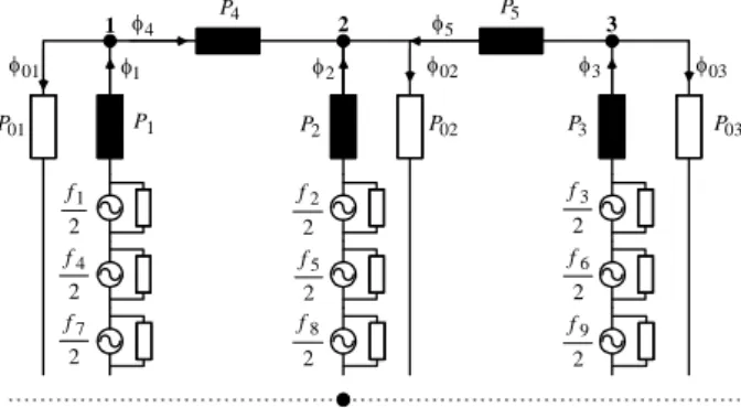
Fig. 1 presents the phase, limb, three-winding, core-type transformer. The unit under study has the particularity of having the highest voltage windings nearest the core. Assuming a slightly greater magnetomo-tive force (MMF) in these windings, a typical flux distri-bution, valid for concentric and non-interleaving wind-ings, is sketched in Fig. 1, which can be classified into the following categories [13,14]:
a) Magnetic fluxes which links windings of the same limb and windings of others limbs, and have a mag-netic path which is mainly confined to the core mate-rial (φi).
b) Leakage fluxes which links only one winding, and have a magnetic path which is mainly confined in the air space between the windings (φσi).
c) Columns leakage fluxes (zero sequence fluxes), which links the windings of the same limb, but fails to link with the windings of other limbs. The mag-netic path for these fluxes is the core limbs and the air surrounding the windings (φ0i).
Based on the flux distribution, and taking advantage of the vertical symmetry of the transformer [19], it is possi-ble to represent the transformer by an equivalent magnetic circuit, Fig. 2, consisting of magnetomotive forces, related with each winding, and lumped permeances, which are di-rectly related to the above defined fluxes. In Fig. 2, the permeances in black correspond to the segments of the magnetic core material (each segment have the same satu-ration level), being non-linear, whereas the white per-meances are related to the air space, being assumed as lin-ear. Under nominal steady-state operation, the leakage re-luctances are several times greater than the magnetic core reluctances, being assumed that they are in parallel with the MMF.
As a first approach, let's consider only the excited windings and neglect the leakage fluxes associated with each winding. In a similar manner to that presented in [19], which consider a five-legged transformer model, the flux-MMF relation (φ-f) can be expressed as:
i i f f f a a a a a a a a a f A⋅ = ⇒ ⎥ ⎥ ⎥ ⎦ ⎤ ⎢ ⎢ ⎢ ⎣ ⎡ ⋅ ⎥ ⎥ ⎥ ⎦ ⎤ ⎢ ⎢ ⎢ ⎣ ⎡ = ⎥ ⎥ ⎥ ⎦ ⎤ ⎢ ⎢ ⎢ ⎣ ⎡ φ φ φ φ 3 2 1 33 23 13 23 22 12 13 12 11 3 2 1 (1) where
(
)
[
P P P P D]
P a 1 1 22 33 232 2 1 11= 1− − (2a) D P P P P a 1 2 12 33 2 1 12 = (2b) D P P P P a 1 3 12 23 2 1 13=− (2c)(
)
[
P P P D]
P a 2 2 11 33 2 1 22= 1− (2d)Fig. 1: Flux distribution in a three-phase, three-limb, three- -winding, core-type transformer.
Fig. 2: Equivalent magnetic circuit.
D P P P P a 2 3 11 23 2 1 23= (2e)
(
)
[
P P P P D]
P a 3 3 11 22 122 2 1 33= 1− ⋅ − (2f) 2 12 33 2 23 11 33 22 11 P P P P P P P D= A= ⋅ ⋅ − ⋅ − ⋅ (2g) and 01 4 1 11 P P P P = + + (3a) 4 12 P P =− (3b) 02 5 4 2 22 P P P P P = + + + (3c) 5 23 P P =− (3d) 03 5 3 33 P P P P = + + (3e)The nodal MMF's between each node and the n point
of the equivalent circuit become:
⇒ ⎥ ⎥ ⎥ ⎦ ⎤ ⎢ ⎢ ⎢ ⎣ ⎡ ⋅ ⎥ ⎥ ⎥ ⎦ ⎤ ⎢ ⎢ ⎢ ⎣ ⎡ ⋅ ⎥ ⎥ ⎥ ⎦ ⎤ ⎢ ⎢ ⎢ ⎣ ⎡ = ⎥ ⎥ ⎥ ⎦ ⎤ ⎢ ⎢ ⎢ ⎣ ⎡ − 3 2 1 3 2 1 1 33 23 23 22 12 12 11 3 2 1 0 0 0 0 0 0 0 0 2 1 f f f P P P P P P P P P P f f f n n n i in B f f = ⋅ ⇒ (4)
from which the yoke fluxes can be computed:
(
f n f n)
P4 1 2 4 = − φ (5)(
f n f n)
P5 3 2 5 = − φ (6) 01 φ φ02 2 φ 4 φ φ5 03 φ 1 σ φ 4 σ φ 7 σ φ 2 σ φ 5 σ φ 8 σ φ 6 σ φ 3 σ φ 9 σ φ 1 φ φ3 3 φ 2 φ 1 φ 4 φ φ5 01 φ φ02 φ03 2 1 f 2 4 f 2 7 f 4 P P5 2 2 f 2 5 f 2 8 f 1 2 3 n 01 P P1 P2 P02 P3 P03 2 3 f 2 6 f 2 9 fRecognising that f =N1i and λ=N1φ, the main linkage fluxes, which do not take into account the leakage fluxes, can be expressed, from (1), as:
w
w A i
λ p = 2 ⋅
1
N (w=1,2,3) (7) The total linkage fluxes can now be computed, introduc-ing the leakage fluxes, as follows:
w w w w w λ L i L i λ = p + σ ⋅ = ⋅ (w=1,2,3) (8)
being Lσw the diagonal leakage inductance matrix.
2.2. Electric Equivalent Circuit
For the Ynzn5 connection, the electric equivalent
cir-cuit is shown in Fig. 3, assuming a three-phase balanced resistor load. The equations that describe the terminal conditions at each winding can be expressed as:
dt d w w w w R i λ v = ⋅ + (w=1,…,9) (9)
From the inspection of Fig. 3, it follows that:
⎪ ⎩ ⎪ ⎨ ⎧ ⋅ − = − = ⋅ − = − = ⋅ − = − = 6 9 4 5 8 6 4 7 5 L L cn L L bn L L an i R v v v i R v v v i R v v v (10a) ⎪ ⎩ ⎪ ⎨ ⎧ = = = 3 3 2 2 1 1 i i i i i i L L L ⎪ ⎩ ⎪ ⎨ ⎧ − = = − = = − = = 9 4 6 8 6 5 7 5 4 i i i i i i i i i L L L (10b)
Using (9) and (10) the following differential equation is obtained: L w v R i λ ⋅ − = ∗ dt d (11) where:
[
]
T ) ( ) ( ) ( ... ... 9 4 8 6 7 5 3 2 1 λ − λ λ − λ λ − λ λ λ λ = ∗ w λ (12)[
]
T Cn Bn An v v v 0 0 0 = v (13)]
) 2 ( ) 2 ( ) 2 ( ... ... diag L s L s L s R R R R R R p R p R p R + + + ⎢⎣ ⎡ = R (14)[
]
T L L L L L L i i i i i i 1 2 3 4 5 6 = L i (15)being Rp and Rs the primary and secondary winding
resis-tances, respectively.
In order to maintain a trade off between complexity and accuracy, an approximation was made to include the excitation losses, connecting three linear resistance branches across the terminals of the excited windings.
Fig. 3: Ynzn5 connection.
2.3. Resultant Coupled Electromagnetic Model
When the transformer's secondary is loaded there are three MMF's in each limb. It is now necessary to expand
(1), as follows: ⎥ ⎥ ⎥ ⎦ ⎤ ⎢ ⎢ ⎢ ⎣ ⎡ − + − + − + ⋅ ⎥ ⎥ ⎥ ⎦ ⎤ ⎢ ⎢ ⎢ ⎣ ⎡ = ⎥ ⎥ ⎥ ⎦ ⎤ ⎢ ⎢ ⎢ ⎣ ⎡ φ φ φ 6 2 5 2 3 1 5 2 4 2 2 1 4 2 6 2 1 1 33 23 13 23 22 12 13 12 11 3 2 1 L L L L L L L L L i N i N i N i N i N i N i N i N i N a a a a a a a a a (16)
which leads to:
∗ ⋅ = w L Γ λ i (17) where: 1 66 56 46 36 26 16 56 55 45 35 25 15 46 45 44 34 24 14 36 35 34 33 23 13 26 25 24 23 22 12 16 15 14 13 12 11 − ⎥ ⎥ ⎥ ⎥ ⎥ ⎥ ⎥ ⎥ ⎦ ⎤ ⎢ ⎢ ⎢ ⎢ ⎢ ⎢ ⎢ ⎢ ⎣ ⎡ = L L L L L L L L L L L L L L L L L L L L L L L L L L L L L L L L L L L L Γ (18) with: 1 11 2 1 11=N a +Lσ L (19) 12 2 1 12 N a L = (20) 13 2 1 13 N a L = (21) ) ( 12 11 2 1 14 N N a a L = − (22) ) ( 13 12 2 1 15 N N a a L = − (23) ) ( 11 13 2 1 16 N N a a L = − (24) 2 22 2 1 22=N a +Lσ L (25) 23 2 1 23 N a L = (26) ) ( 22 12 2 1 24 N N a a L = − (27) ) ( 23 22 2 1 25 N N a a L = − (28) ) ( 12 23 2 1 26 N N a a L = − (29) 3 33 2 1 33=N a +Lσ L (30) ) ( 23 13 2 1 34 N N a a L = − (31) 1 v 2 v 3 v 1 L i 2 L i 3 L i 4 v 5 v 6 v 4 i 5 i 7 v 8 v 9 v 8 i 6 i i9 7 i iL4 5 L i 6 L i A B C n a b c n n an v bn v cn v 1 i 2 i 3 i L R L R L R
) ( 33 23 2 1 35 N N a a L = − (32) ) ( 13 33 2 1 36 N N a a L = − (33) 7 5 11 12 22 2 2 44 =N (a −2a +a )+Lσ +Lσ L (34) ) ( 23 22 13 12 2 2 45 N a a a a L = − − + (35) ) ( 12 23 11 13 2 2 46 N a a a a L = − − + (36) 8 6 22 23 33 2 2 55=N (a −2a +a )+Lσ +Lσ L (37) ) ( 13 33 12 23 2 2 56 N a a a a L = − − + (38) 9 4 33 13 11 2 2 66 =N (a −2a +a )+Lσ +Lσ L (39)
The influence of the no-load losses conductances, Gfe,
can now be introduced in (17):
v G λ Γ
iL = ⋅ w∗ + fe⋅ (40)
being Gfe a 6×6 matrix, where only the first 3×3 diagonal sub-matrix has non-zero values [4].
2.4. Algorithm
Since the inductances depend on the fluxes, a predic-tor-corrector algorithm is used. First, by using the induc-tance matrix calculated in the previous iteration, the link-age fluxes are obtained:
[
]
∗ ∗ ⋅ ⋅ − ⋅ ⋅ − = fe w w I R G v RΓ λ λ dt d (41) being I a 6×6 identity matrix.Afterwards, the main linkage fluxes are derived, using (8), and subsequently, the fluxes in the columns are com-puted. Next, the MMF's are obtained, from the inverse
form of (1), and the nodal MMF's, from (4). With the
nodal MMF's, the yoke fluxes are determined, through (5)
and (6), and then the permeances are evaluated. The in-ductance matrix can now be updated and the currents are obtained through (40).
2.5. Model Parameters Definition
The following procedures for the model parameters definition is based on the assumption that no geometrical, magnetic and electrical data are available, and all the pa-rameters have to be evaluated, which, otherwise, repre-sents a quite common situation in the real industrial envi-ronment.
The windings and the no-load losses resistances are obtained through a DC test and a conventional open-circuit test, respectively.
It is assumed that there is an individual leakage induc-tance associated with each winding, which is determined from the conventional single-phase short-circuit test, were
lσp= lσs= lcc/2 (p.u.). Additionally, it can be found that the
short-circuit inductance, obtained from a three-phase short-circuit test, for the case of the Ynzn5 connection, is
very close to lσp +2lσs (p.u.), in accordance to the flux
dis-tribution of Fig. 1. Moreover, the non-standard tests pro-posed in [21] also confirm the computed values.
The non-linear permeances are obtained by the follow-ing expression:
l A
P=μ fe (42)
were Afe is the effective iron cross-sectional area and l is
the mean-length of the transformer segment under consid-eration. More specifically, for the permeances of Fig. 2, l
is the half length of the limbs and the full mean-length of the yoke segments, due to the vertical symmetry of the transformer [19]. To obtain the effective iron cross-sectional area, the geometrical dimensions of the core are to be affected by a lamination factor of 0.95 [16, 22].
The B-H curve can be obtained by performing a non-standard open-circuit test, in which one winding of each lateral limb has to be excited in equal but in opposite di-rections, in order to force the flux in the central limb to be zero [15, 16]. The resultant voltage and currents wave-forms have to be digitally acquired, for a high level of saturation, from which the B-H characteristic can be
evaluated. The ideal magnetic characteristic of the mate-rial can be determined from the mean line of the hysteresis loop [23]. A 10th-order polynomial is used to accurately fit the μ-B relationship, obtained from the ideal B-H curve. Therefore, the non-linear permeances can be com-pletely defined.
On the other hand, a zero-sequence series test, at low saturation level, provides the values for the linear per-meances P01, P02 and P03 [16].
3. MODEL VALIDATION
For the model validation a three-phase, three-limb transformer, of 6 kVA, 220/127 V, was used. The trans-former has four-windings per limb, although only three of them are used for the case of the Ynzn connection. The
primary winding and one of the two secondary windings, per limb, were modified by addition of a number of tap-pings connected to the coils, allowing for the introduction of different percentages of shorted turns at several loca-tions in the winding, for subsequent studies of inter-turn short-circuits occurrence [3].
The transformer model, for the case of a Ynzn5
con-nection, was tested under steady-state load conditions. A three-phase, star connected, balanced resistor of 96 Ω per phase, was coupled to the secondary side, being the pri-mary side energised by a three-phase voltage system, at the transformer nominal values.
in2 iL4 iL5 iL6 in2 iL4 iL5 iL6 in1 iL1 iL2 iL3 in1 iL1 iL2 iL3 primary secondary primary secondary
The harmonic characteristics of the transformer excita-tion currents are significantly different under non-sinusoidal input voltages as compared to the non-sinusoidal supply voltages case [24]. Additionally, under load operat-ing conditions, the harmonic content of the supply volt-ages also affects, in a minor extent, all the current wave-forms. Therefore, both harmonic magnitudes and har-monic phases of the supply voltages were taken into ac-count in the conducted simulation study.
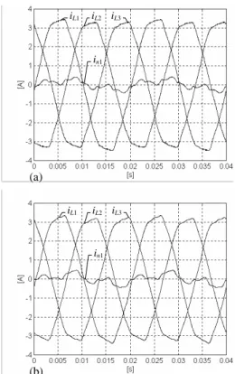
The experimental and simulated primary side currents waveforms are shown in Fig. 4(a) and Fig. 4(b), respec-tively, which are shown to be in relatively good agree-ment. The neutral current has a dominant third harmonic component, which is primarily due to the saturation ef-fects.
The experimental and simulated secondary side cur-rents waveforms, presented in Fig. 5(a) and Fig. 5(b), re-spectively, are also shown to be in good agreement. For this type of connection, and due to the flattened supply voltages, the secondary currents present peaked wave-forms. Since the supply voltages and the load resistors are approximately balanced, the magnitudes of both experi-mental and simulated secondary neutral currents are neg-ligible.
The experimental primary side current Park’s Vector pattern, under steady-state load conditions, shown in Fig 6(a), differs slightly from the circular locus expected
(a)
(b)
Fig. 4: Primary side currents waveforms for the case of a
Ynzn5 connection and a pure resistive load:
(a) experimental; (b) simulated.
for ideal conditions, due to, among others, the supply voltage harmonic content and the minor reluctance seen from the central limb, with respect to the lateral limbs. The corresponding simulated Park's Vector pattern, shown in Fig. 6(b), is in relatively good agreement with the ex-perimental one. The exex-perimental and simulated secon-dary side current Park’s Vector patterns are also shown in Fig. 6(a) and Fig. 6(b), respectively.
By performing the pertinent modifications in the elec-tric equivalent circuit, it would be possible to study any other three-phase electrical connection, including auto-transformers. The cases of Ynyn, Yyn and Dyn transformer connections were also implemented, which yield good re-sults.
(a)
(b)
Fig. 5: Secondary side currents waveforms for the case of a
Ynzn5 connection and a pure resistive load:
(a) experimental; (b) simulated.
(a) (b)
Fig. 6: Primary and secondary side currents Park's Vector pat-terns for the case of a Ynzn5 connection and a pure
4. CONCLUSIONS
This paper describes the development and implementa-tion of a coupled electromagnetic model for the case of a three-phase, three-leg, three-winding transformer, with a
Ynzn connection. The model is based on the simultaneous
analysis of both magnetic and electric lumped-parameters equivalents circuits, which allows to define and simulate the transformer in its natural technology. Furthermore, with this approach, it is possible to manipulate the wind-ings composition, which constitutes an essential requisite for the study of inter-turn short-circuit faults.
All the parameters required for the model can be evaluated from experimental tests and from the relative dimensions of the core, which are usually available. The
Ynzn connected transformer model was validated under
steady-state load conditions. Both simulation and experi-mental tests results demonstrate the adequacy of the model, under normal operating conditions.
Further work is currently in progress, concerning the modelling and simulation of the behaviour of three-phase transformers, under the influence of winding inter-turn short-circuit faults. Additionally, some refinements of the proposed model will be introduced, with the aim of deal-ing with the simultaneous occurrence of winddeal-ing faults, unbalanced supply voltages, unbalanced loads, or even the surrounding presence of power electronics equipment.
ACKNOWLEDGEMENT
The authors wish to acknowledge the financial support of the Portuguese Foundation for Science and Technol-ogy, under Project Number PRAXIS/P/EEI/14151/1998.
REFERENCES
[1] S. Aubertin, Opportunity knocks, International Power
Generation, 20(2), 1997, 47-48.
[2] E. Blauvert, Report on high voltage power transformers,
Power Engineering International, 8(1), 2000, 18-20.
[3] A. J. M. Cardoso and L. M. R. Oliveira, Condition moni-toring and diagnostics of power transformers, International
Journal of COMADEM, 2(3), 1999, 5-11.
[4] L. M. R. Oliveira and A. J. M. Cardoso, Modelling and simulation of three-phase power transformers, Proceedings of the 6th International Conference ELECTRIMACS 99, Lisbon, Portugal, vol. 2/3, 1999, 257-262.
[5] H. W. Dommel, Transformer models in the simulation of electromagnetic transients, Proceedings of the 5th Power Systems Computation Conference, Cambridge, England, Paper 3.1/4, 1975.
[6] V. Branwajn; H. W. Dommel and I. I. Dommel, Matrix representation of three phase N-winding transformers for steady-state and transient studies, IEEE Trans. Power
Ap-par. & Syst., 101(6), 1982, 1369-1378.
[7] E. P. Dick and W. Watson, Transformer models for tran-sients studies based on field measurements, IEEE Trans.
Power Appar. & Syst., 100(1), 1981, 409-417.
[8] C. M. Arturi, Transient simulation and analysis of a three-phase five-limb step-up transformer following an out-of-phase synchronization, IEEE Trans. PWRD, 6(1), 1991, 196-203.
[9] G. R. Slemon, Magnetoelectric devices: transducers,
trans-formers and machines, (New York, John Wiley & Sons,
1966).
[10] A. Narang and R. H. Brierley, Topology based magnetic model for steady-state and transient studies for three-phase core type transformers, IEEE Trans. on Power Systems, 9(3), 1994, 1337-1349.
[11] X. Chen and S. S. Venkata, A three-phase three-winding core-type transformer model for low-frequency transient studies, IEEE Trans. PWRD, 12(2), 1997, 775-782. [12] B. A. Mork, Five-legged wound-core transformer model:
derivation, parameters, implementation and evaluation,
IEEE Trans. PWRD, 14(4), 1999, 1519-1526.
[13] R. Yacamini and H. Bronzeado, Transformer inrush calcu-lations using a coupled electromagnetic model, IEE Proc.
Sci. Meas. Technol., 141(6), 1994, 491-498.
[14] W. K. Macfayden; R. R. S. Simpson; R. D. Slater and W. S. Wood, Method of predicting transient-current patterns in transformers, Proc. IEE, 120(11), 1973, 1393-1396. [15] H. L. Nakra and T. H. Barton, Three phase transformer
transients, IEEE Trans. Power Appar. & Syst., 93(6), 1974, 1810-1819.
[16] M. Elleuch and M. Poloujadoff, Three phase, three limb transformer model for switching transient calculations. Part I: Parameter definition and identification, Acta Technica
Csav, 1, 1988, 100-117.
[17] M. Elleuch and M. Poloujadoff, Three phase, three limb transformer model for switching transient calculations. Part II: Study of inrush currents for symmetrical and unsymmet-rical connections, Acta Technica Csav, 2, 1988, 196-207. [18] M. Elleuch and M. Poloujadoff , A contribution to the
modelling of three phase transformers using reluctances,
IEEE Trans. on Magnetics, 32(2), 1996, 335-343.
[19] X. S. Chen and P. Neudorfer, Digital model for transient studies of a three-phase five-legged transformer, IEE Proc.
Pt. C, 139(4), 1992, 351-359.
[20] X. Chen, A three-phase multi-legged transformer model in ATP using the directly-formed inverse inductance matrix,
IEEE Trans. PWRD, 11(3), 1996, 1554-1562.
[21] O. G. C. Dahl, Electric circuits, theory and applications,
Vol. I: Short-circuit currents and steady-state theory, (New
York, McGraw-Hill Book Company, Inc., 1928).
[22] J. M. Prousalidis; N. D. Hatziargyriou and B. C. Papadias, The geometrical transformer model: Parameter estimation method, 21st EMTP Users Group Meeting, Greece, 1992. [23] I. Marongiu and E. Pagano, I Transformatori (appunti dalle
lezioni), (Napoli, Liguori Editori, 1994, in Italian).
[24] A. H . Chowdhury; W. M. Grady and E. F. Fuchs, An in-vestigation of the harmonic characteristics of transformer excitation current under nonsinusoidal supply voltage,