Three-phase phononic materials
R. Cimrman
a,∗, E. Rohan
aa
Department of Mechanics & New Technologies Research Centre, Faculty of Applied Sciences, University of West Bohemia, Univerzitn´ı 22, 306 14 Plzeˇn, Czech Republic
Received 29 September 2008; received in revised form 25 February 2009
Abstract
We consider a strongly heterogeneous material consisting of three phases: an elastic matrix, medium-size inclu-sions periodically embedded in the elastic matrix; these incluinclu-sions are constituted by small rigid incluinclu-sions coated by a very compliant material. The dependence on scale of elasticity coefficients of the deformable medium-size inclusions is treated in the context of linear elasticity by the homogenization procedure providing a limit model that inherently describes band gaps in acoustic wave propagation. The band gaps occur for certain intervals of long wavelengths for which a frequency-dependent “mass density” tensor is negative. We illustrate the theoretical results with numerical simulations.
c
2009 University of West Bohemia. All rights reserved.
Keywords:three-phase material, homogenization, rigid inclusion, acoustic band gaps
1. Introduction
We present an approach to modelling the phononic materials. These materials are similar to better known photonic crystals, cf. [4, 8, 13], but the main interest lies in modelling the propa-gation of elastic waves instead of light waves. Both the phononic and photonic materials exhibit forbidden frequency ranges of incident waves, for which the sound/light waves cannot propa-gate: the structure is blocked from free vibrations. In the context of sound wave propagation the forbidden frequency ranges are calledacoustic band gaps. This wave dispersion feature has a lot of serious practical applications, such as acoustic wave guides, or silencers. Such smart materials are already being produced and their properties experimentally verified, cf. [11]; this raises the need for proper modelling tools able to predict their behaviour.
In this article we treat a strongly heterogeneous material consisting of three phases: an elastic matrix, medium-size inclusions periodically embedded in the elastic matrix; these inclu-sions are constituted by small rigid incluinclu-sions coated by a very compliant material (rubber, or epoxy resin). Considering the rigid inclusions is a new contribution and generalizes the two-phase material analyzed in [2, 3, 10]. The elasticity coefficients of the deformable medium-size inclusions depend on the scale. This is treated in the context of linear elasticity by the homog-enization procedure providing a limit homogenized model that inherently describes band gaps in acoustic wave propagation.
The homogenization based prediction of the band gap distribution (i.e. analysis of the effec-tive mass tensor eigenvalues) is relaeffec-tively simple and effeceffec-tive in comparison with the “standard computational approach” based on a finite scale heterogeneous model, which requires to eval-uate all the Brillouin zone for the dispersion diagram reconstruction; as the consequence, it
leads to a killing complexity, namely when the inverse problem (optimal design) is considered. This is the main advantage of the homogenization based two-scale modeling. As an important restriction, this modeling approach is relevant for the long wave propagation, see [10].
We should point out that while band-gaps never occur in homogeneous or weakly hetero-geneous materials, the “homogenized” material is rather a mathematical model of seemingly homogeneous material with “hidden” components — the underlying heterogeneous structure responsible for the dispersion is inherited by the model in terms of its effective parameters (the inertia mass and elasticity); this was discussed newly in [9], where a “generalized” Newton’s second law was presented.
The model proposed in Section 3 is implemented in our open-source software SfePy, [5]. Numerical examples are presented in Section 5; mainly the influence of the rigid inclusion size on the band gap distribution is shown.
2. Problem setting
We consider a strongly heterogeneous material occupying an open bounded domainΩ ⊂ R3 consisting of three phases, see Fig. 1. The first phase is an elastic matrix, the second phase corre-sponds to medium-size inclusions periodically embedded in the elastic matrix. These inclusions themselves are constituted by small rigid inclusions coated by a very compliant material (rub-ber). The rigid inclusions represent the third phase. The domainΩis constituted as a periodic lattice structure generated by unit periodic reference cellY =]0,1[3 scaled byε. The rigid in-clusionY3⊂Y has the boundaryΓ3and is coated byY2, so thatY2∩Y3=∅and(Y2∪Y3)⊂Y,
Y2∩Y3= Γ3; the matrix part isY1=Y \(Y2∪Y3), see Fig. 2. We denoteY2+3=Y \Y1.
Fig. 1. Strongly heterogeneous material Fig. 2. Periodic reference cell
In Section 2.1 we define the three-phase strongly heterogeneous medium (SHM), then in Section 2.2 we recall the equations governing stationary waves in SHM developed in [10], and finally, in Section 3 we describe the resulting homogenized model, also based on results in [10].
2.1. Strongly heterogeneous material
The material properties, being attributed to material constituents of the three phases, vary pe-riodically with position. Throughout the text all quantities varying with this microstructural periodicity are denoted with superscriptε. Using the reference cellY we generate the decom-position ofΩas follows
Ωε 2 =
k∈Kε
ε(Y2+k), whereKε={k∈Z|ε(k+Y2)⊂Ω},
Ωε 3 =
k∈Kε
ε(Y3+k), Ωε1= Ω\(Ωε2∪Ωε3),
so thatΩ = Ωε
Properties of a three dimensional body made of the elastic material are described by the elasticity tensorcε
ijkl, wherei, j, k, l= 1,2, . . . ,3. As usual we assume both major and minor symmetries ofcε
ijkl(cεijkl=cεjikl=cεklij).
The key assumption of the modelling is thatthe material densityis comparable in subdo-mainsΩε
2∪Ωε3 andΩε1, while the stiffness coefficients in the medium-size inclusionsΩε2 are significantly smaller than in the matrix Ωε
1. The stiffness of the small inclusionsΩε3 is much higher than in Ωε
2 so that it can be considered as rigid. In reality, stiffness of a material is corelated with its mass. Thus, because of small density of the material inΩε
2, the role ofΩε3is an added mass so that the assumption of comparable densities inΩε
2∪Ωε3 andΩε1 is fulfilled. Thestrong heterogeneityis related to the geometrical scale of the underlying microstructure by coefficientε2, as follows:
ρε(x) =
⎧ ⎨
⎩
ρ1 inΩε 1,
ρ2 inΩε 2,
ρ3 inΩε 3,
cε ijkl(x) =
⎧ ⎨
⎩
c1
ijkl inΩε1,
ε2c2
ijkl inΩ ε 2,
(1/ε2)c3
ijkl inΩε3,
(1)
whereρ3 ≫ρ2. We shall consider positive densities: let0< ρ, ρ∈
R, we assumeρ < ρε(x)<
ρa.e. inΩ. Further, we assume standard ellipticity and boundedness of the elastic coefficients: letS+be the set of all symmetric real second order tensors in
R3, then∀eij,eˆij ∈S+,∃μ, μ >0 such that
μ eijeij≤cαijkleijekl and cαijkleijeˆkl≤μ eijeˆij, α= 1,2,3. (2)
2.2. Modelling the stationary waves
We consider a stationary wave propagation in the SHM, see [10]. For simplicity we restrict the model to the description of clamped structures loaded by volume forces. Let us assume harmonic single-frequency volume forces,
F(x, t) =f(x)eiωt, (3)
where f = (fi), i = 1,2,3 is the local amplitude and ω is the frequency. We consider a dispersive displacement field with the local magnitudeuε
Uε(x, ω, t) =uε(x, ω)eiωt. (4)
This allows us to study the steady periodic response of the medium, as characterized by the displacement fielduεwhich satisfies the following boundary value problem:
−ω2ρε
uε−divσε=f inΩ,
uε= 0 on∂Ω, (5)
where the stress tensorσε= (σε
ij)is expressed in terms of the linearized strain tensoreε= (eεij) by the Hooke’s lawσε
ij =c ε
ijklekl(uε). The problem (5) can be formulated in the weak form as follows: Finduε∈H1
0(Ω)such that
−ω2
Ω
ρε uε·v+
Ω
cε
ijklekl(uε)eij(v) =
Ω
f·v for allv∈H10(Ω), (6)
whereH1
3. Homogenized model
We wish to associate the SHM model (6) with a homogeneous model relevant to the macro-scopic scale. For this taskmethods of homogenizationare widely accepted. Due to thestrong heterogeneityin the elastic coefficients the homogenized model exhibits dispersive behaviour; this phenomenon cannot be observed when standard two-scale homogenization procedure is applied to a medium with scale-independent material parameters, as pointed out in [1]. In [3] the unfolding operator method of homogenization [6, 7] was applied with the strong hetero-geneity assumption (1); it can be shown thatuε →uasε→0, whereuis the “macroscopic” displacement field describing behaviour of the homogenized medium. Here we just record the resulting system of coupled equations which describe the structure behaviour at two scales, the “macroscopic” one and the “microscopic” one, since the theoretical considerations remain the same as in [10].
First we define the homogenized coefficients involved in the homogenized model of wave propagation. The “frequency-dependent coefficients” are determined just by material properties of the inclusion Y2+3 and by the material densityρ1, whereas the elasticity coefficients are related exclusively to the matrix compartmentY1.
Frequency-dependent homogenized coefficients involved in the macroscopic momentum equation are expressed in terms of eigenelements of the following spectral problem.
3.1. Spectral problem
Let us define a space of functions that describerigid body motions(RBM) inY3and are zero on the boundary ofY2+3:
S0(¯y, Y3, Y2+3) ={v∈H01(Y2+3)| ∃(¯sij,¯v) : vi= ¯vi+ ¯sij(yj−y¯j), ∀y∈Y3}, (7)
where(¯sij,¯v)is the spin–translation couple and¯yis the barycentre ofY3. We shall employ the following notation:
aYm(u,v) =
Ym
cm ijkle
y kl(u)e
y ij(v),
̺Ym(u,v) =
Ym
ρm u·v,
form= 2,3. The spectral problem for eigenelements(λr,ϕr) ,λr∈
R,ϕr ∈S
0(¯y, Y3, Y2+3), noting thataY3(ϕ
r,v)≡0due to RBM constraint inY3, is:
aY2(ϕ
r,
v) =λr[̺ Y2(ϕ
r,
v) +̺Y3(ϕ
r,
v)] , ∀v∈S0(¯y, Y3, Y2+3), (8)
where
̺Y2(ϕ
r,ϕs) +̺ Y3(ϕ
r, ϕs) =δ
rs. (9)
It is easy to see that the orthogonality in (9) holds and0 < λr ∈
R; indeed,aY2(·,·)is the
elliptic bilinear form onH1(Y). In the sequel we shall need theeigenmomentummr= (mr i),
mr=
Y2
ρ2ϕr+
Y3
3.2. Homogenized coefficients
The homogenized coefficients can be computed in much the same way, as it was done for just two-phase composite, cf. [3, 10], when the role of Y2 is substituted by the unionY2+3. We recover the following tensors, all depending onω2:
• mass tensorM∗ = (M∗
ij)
M∗
ij(ω 2) = 1
|Y|
Y
ρδij−
1
|Y|
r≥1
ω2
ω2−λrm r im
r
j ; (11)
• applied load tensorB∗= (B∗
ij)
B∗
ij(ω 2) =δ
ij−
1
|Y|
r≥1
ω2
ω2−λrm r i
Y2
ϕr
j . (12)
The elasticity coefficientsare related to the perforated matrix domain, thus being indepen-dent of the inclusions material:
C∗
ijkl=
1
|Y|
Y1
c1 pqrse
y rs(w
kl+Πkl)e
pq(wij+Πij), (13)
whereΠkl= (Πkl
i) = (ylδik)andwkl∈H1#(Y1)are the corrector functions satisfying
Y1
c1 pqrse
y rs(w
kl+Πkl)ey
pq(v) = 0 ∀v∈H1#(Y1). (14)
AboveH1#(Y1)is the restriction ofH1(Y1)to the Y-periodic functions (periodicity w.r.t. the
homologous points on the opposite edges of∂Y).
3.3. Macromodel
The global equation— the macromodel — involves the homogenized coefficients. We find u∈H1
0(Ω)such that
−ω2
Ω
(M∗(ω2)·u)·v+
Ω
Cijkl∗ ekl(u)eij(v) =
Ω
(B∗(ω2)·f)·v, ∀v∈H1
0(Ω). (15)
Heterogeneous structures with finite scale of heterogeneities exhibit the frequencyband gaps for certain frequency bands. As the main advantage of this homogenized model, by analyzing the dependenceω→M∗(ω)one can determine distribution of the band gaps with significantly less effort than in case of analyzing them in the standard way, see e.g. [12]. In [10] an exhaustive description of band gaps computations is given, some of which is summarized in Section 4.
4. Band gaps
In the context of our homogenization-based modelling of phononic materials, the band gaps are frequency intervals for which the propagation of waves in the structure is disabled or restricted in the polarization.
1. propagation zone— all eigenvalues ofM∗
ij(ω)are positive: then homogenized model (15) admits wave propagation without any restriction of the wave polarization;
2. strong band gap– all eigenvalues ofM∗
ij(ω)are negative: then homogenized model (15) doesnotadmit any wave propagation;
3. weak band gap— tensorM∗
ij(ω)is indefinite, i.e. there is at least one negative and one positive eigenvalue: then propagation is possible only for waves polarized in a manifold determined by eigenvectors associated with positive eigenvalues. In this case the notion of wave propagation has a local character, since the “desired wave polarization” may depend on the local position inΩ.
We denote the smallest and the highest eigenvalues of M∗
ij(ω)byγ
▽(ω)andγ△(ω),
respec-tively.
4.1. Computing the band gaps
Distribution of the band gaps is based on analyzing the eigenvalues of tensorM∗(ω)
which is a nonlinear function (11) of ω. Therefore, in general, it can be done numerically using a finite element (FE) approximation of eigenvalue problem (8), see Section 4.2. Thus we obtain a finite numbernhof the approximated eigenvalues and their associated eigenfunctions(λr,φr),
r= 1, . . . , nh; herenhis the number of free displacement degrees of freedom (dofs) for a given FE mesh.
From the theoretical analysis of a similar homogenized “phononic” problem, which was done for rectangular domainY2and the Laplace operator it follows that the homogenized coef-ficient analogous to the mass tensor (11) is expressed in terms of series containing integrals of the type (10), which vanish “exactly” for some modes. Due to this let us define theeigenmode cut-off thresholdc >0and introduce theset of non-zero modes
Ih(c)≡ {1≤k≤nh| |mkh|> c}, (16)
wheremk
his evaluated according to (10), i.e.
mkh=
Y2,h
ρ2φr+
Y3,h
ρ3φr.
(17)
Then, denoting the averaged densityρ¯, the homogenized mass tensor is computed by
M∗
ij(ω) =δijρ¯−
ω2 |Y|
k∈Ih(c) 1
ω2−λkm k
i,hmkj,h, i, j= 1,2,3. (18)
4.2. Discrete eigenvalue problem: enforcing RBM constraints
The FE-discretized counterpart of (8) is to seek(λr,φr
),λr∈
R,φr∈Sh0(¯y, Y3, Y2+3)and
vTAφr
=λrvTMφr
, ∀v∈Sh0(¯y, Y3, Y2+3), (19)
Let us assume to have the standard matricesA¯, M¯, corresponding to FE-discretized
op-eratorsaY2(u, v)and̺Y2+3(u,v), such that the fixed zero displacements onΓ2+3are already
eliminated. Correspondingly, let us define alsov¯,φ¯. To enforce the RBM constraint the
fol-lowing splitting can be used:
¯ v=
v
f
vr , A¯ =
A
f f Af r
Arf Arr , (20)
where the suffixf relates to the free dofs andrto the RBM-constrained dofs. Analogously we split alsoφ¯,M¯. The constrained dofs in a pointycan be expressed as
vr(y) =
⎡
⎣
0 y3 −y2 1 0 0
−y3 0 y1 0 1 0
y2 −y1 0 0 0 1
⎤
⎦
θ
v0 ≡R(y)θ+Iv0≡T(y)s, (21)
wheres =
θ v0 T
, R(y)θ is a linearized rotation ofy w.r.t. 0 by a spinθ andv0 is a
translation. In 2D,R(y)θ≡
−y2 y1 T
θandθis a scalar. Repeating this for each FE mesh node, we can writevr=Ts,φr=Tr. The eigenvalue problem (19) can thus be written as
vT f s
TTT A
f f Af r
Arf Arr
φf
Tr =λ
r vT f s
TTT M
f f Mf r
Mrf Mrr
φf
Tr . (22)
The multiplications by the constraint matrixTcan now be carried out to arrive at (19) with
v=
v
f
s , φ=
φf
r , A=
A
f f Af rT
TTA
rf TTArrT ,
M=
M
f f Mf rT
TTM
rf TTMrrT . (23)
5. Numerical examples
The numerical examples presented below were computed using our finite element code SfePy, [5], that is freely available at http://sfepy.org. Changes in the band gap distribution due to
1. varying the cut-off thresholdc,
2. symmetry / nonsymmetry of the rigid inclusionY3 placement inY2+3, and thus also the underlying FE mesh,
3. varying the size of the rigid inclusionY3
are shown. In all the examples the domainY ∈R2was[−1,1]2, andY
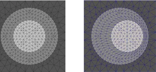
2+3was a circle centered at[0,0]T with radius0.8, see Fig. 3. Material properties were defined as follows:
material subdomain Lam´e coefficients [1010Pa] density [104kg/m3] aluminium Y1 λ1= 5.898,μ1= 2.681 ρ1= 0.2799
epoxy Y2 λ2= 0.1798,μ2= 0.148 ρ2= 0.1142 lead Y3 λ3= 4.074,μ3= 0.5556 ρ3= 1.1340
The FE-discretized eigenvalue problem (8) was solved inY2+3with the clamped boundary
∂Y2+3 (= ∂Y¯2 ∩∂Y¯3) and with the RBM constraint in Y3, see Section 4.2. The computed eigenvalues and eigenvectors(λr,φr)
were then used to construct the mass tensorM∗(ω)given by (18) and to evaluate the band gap distribution for a given frequency range according to the signs of the eigenvalues ofM∗(ω), see Section 4. The eigenmomentum cut-off thresholdcwas
chosen as
c= 0.1 max
k=1...nh |mkh|,
with exception of Section 5.1, where it was the subject of a parametric study. Similarly, the radius of the rigid inclusion wasr(Y3) = 0.45with exception of Section 5.3.
Note: When plotting the eigenvaluesγ▽(ω),γ△(ω)we transform them byarctanfunction
to zoom to the interesting behaviour near zero.
Fig. 3. FE meshes; left: symmetricY2+3, right: shiftedY3. The eigenvalue problem is computed in the circular domainY2+3only
5.1. Cut-off threshold
Forf ∈[0,25]kHz we have conducted a parametric study by settingc= 10qmax
k=1...nh|m
k h| forq = −3 + 0.5j,j = 0, . . . ,6using the mesh with unsymmetricY3 placement, see Fig. 3 (right). In this case we hadnh= 307eigenmomenta out of which the following numbers were under threshold:
j 0 1 2 3 4 5 6
masked 28 104 222 285 301 305 306
The resulting band gaps andγ▽(ω)
,γ▽(ω)
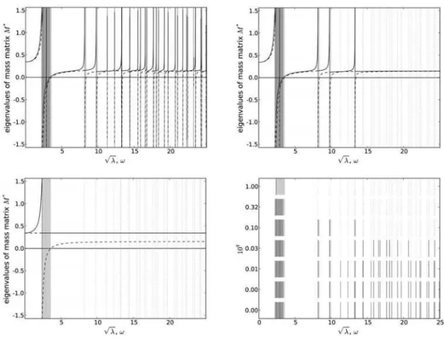
plots are shown in Fig. 4 forj = 0,4,6. It can be seen that forj= 4, i.e.c= 0.1 maxk=1...nh|m
k
h|the band gaps are almost the same as forj= 0, but the spurious oscillations inγ▽(ω),γ▽(ω)are removed. These results support our choice of
cin the other examples.
5.2. Inclusion symmetry
Fig. 4. Band gap distribution; top left: j = 0, top right: j = 5, bottom left: j = 10, bottom right: overview for allq=−3 + 0.5j,j= 0, . . . ,6;arctanγ▽(ω): dashed lines,arctanγ△(ω): solid lines, strong band gaps: gray, weak band gaps: light gray, propagation zone: white, resonance frequencies: solid vertical lines, resonance frequencies masked byc: dotted vertical lines
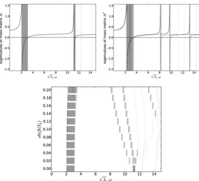
material too. For f ∈ [0,15]kHz a sequence of simulations was performed, starting with a perfectly symmetric shape, see Fig. 3 (left). The rigid inclusionY3was then shifted in steps of 0.02 along thexaxis up to the final position (shift = 0.2) depicted in Fig. 3 (right).
As predicted, no weak band gaps appear in Fig. 5 (top left), corresponding to the symmetric shape, as opposed to Fig. 5 (top right), corresponding to the most shifted Y3. All the cases, including the intermediateY3positions, are summarized in Fig. 5 (bottom).
5.3. Size of the rigid inclusion
The sizes of the rigid inclusionr(Y3)were varied for both the symmetric and unsymmetricY3 placements, see Fig. 6; the results are summarized in Fig. 7 forf ∈ [0,25]kHz. These results suggest that increasing the inclusion size causes broadening of the band gap corresponding to the lowest eigen-frequency computed by (19), and also growth of the separation between the first and the subsequent band gaps. The latter observation is more pronounced in the symmetric case.
6. Conclusion
Fig. 5. Band gap distribution on two FE meshes; top left: symmetric, bottom: summary for all Y3 positions, top right: max. shift; arctanγ▽(ω): dashed lines,arctanγ△(ω): solid lines, strong band gaps: gray, weak band gaps: light gray, propagation zone: white, resonance frequencies: solid vertical lines, resonance frequencies masked byc: dotted vertical lines
Fig. 7. Band gap distribution for varyingr(Y3); left: symmetric, right: shiftedY3position; strong band gaps: gray, weak band gaps: light gray, propagation zone: white, resonance frequencies: solid vertical lines, resonance frequencies masked byc: dotted vertical lines
from [10] to a three-phase phononic material (elastic matrix, inclusions made of small rigid bodies coated by a very compliant material). Introducing therigid inclusionsinto the model is the main new result of the paper. It was motivated by the need to satisfy the key assumption of the modelling: that the material density has to be comparable in both the matrix and the inclusions, while the stiffness coefficients in the inclusions should be significantly smaller than in the matrix. The rigid inclusions, thus, represent an added mass in the soft (and light) medium-size inclusions.
The principal ingredient of the homogenization procedure is the scale dependence of the elastic coefficients in the mutually disconnected inclusions — this leads to acoustic band gaps due to thenegative effective massphenomenon appearing in the upscaled model.
The main advantage of the homogenization based two-scale modeling lies in the fact, that the homogenization based prediction of the band gap distribution for stationary or long guided waves is relatively simple and effective, cf. [10], in comparison with the “standard computa-tional approach” based on a finite scale heterogeneous model, which requires to evaluate all the Brillouin zone for the dispersion diagram reconstruction; as the consequence, it leads to a killing complexity. Moreover, in [10] a correspondence between our band gap diagrams and the classical dispersion diagrams was discussed.
We demonstrated in several numerical examples that these band gaps can be effectively computed. We studied how the prediction of the band gap distribution changes when varying the rigid inclusion size and other parameters.
Acknowledgements
The work has been supported by the Czech Science Foundation, grant GA ˇCR 101/07/1471, and the Czech Government project 1M06031.
References
[1] J. L. Auriault and G. Bonnet. Dynamique des composites elastiques periodiques.Arch. Mech., (37):269–284, 1985.
[3] A. ´Avila, G. Griso, B. Miara, and E. Rohan. Multi-scale modelling of elastic waves — theoretical justification and numerical simulation of band gaps.Multiscale Modeling and Simulation, SIAM, 2007.
[4] G. Bouchitt´e and D. Felbacq. Homogenization near resonances and artificial magnetism from dielectrics.C. R. Acad. Sci. Paris, Ser. I(339):377–382, 2004.
[5] R. Cimrman et al. SfePy home page. http://sfepy.kme.zcu.cz, http://sfepy.org, 2008.
[6] D. Cioranescu, A. Damlamian, and G. Griso. Periodic unfolding and homogenization.C. R. Acad. Sci. Paris, I(335):99–104, 2002.
[7] A. Damlamian. An elementary introduction to periodic unfolding.GAKUTO International series Math. Sci. Appl., 24:119–136, 2005. Multi scale problems and Asymptotic Analysis.
[8] D. Felbacq and G. Bouchitt´e. Theory of mesoscopic magnetism in photonic crystals.Phys. Rev. Lett., 94:183–902, 2005.
[9] G. W. Milton and J. R. Willis. On modifications of newton’s second law and linear continuum elastodynamics.Proc. R. Soc. A, (483):855–880, 2007.
[10] E. Rohan, B. Miara, and F. Seifrt. Numerical simulation of acoustic band gaps in homogenized elastic composites.accepted to Int. J. Eng. Sci., 2009. doi:10.1016/j.ijengsci.2008.12.003. [11] Ping Sheng, X. X. Zhang, Z. Liu, and Chan C. T. Locally resonant sonic materials.Physica B:
Condensed Matter, 338(1–4):201–205, 2003.
[12] O. Sigmund and J. S. Jensen. Systematic design of phononic band-gap materials and structures by topology optimization.Phil. Trans. R. Soc. London, A(361):1 001–1 019, 2003.