CONTROL AND ESTIMATION ALGORITHMS FOR MULTIPLE-AGENT SYSTEMS

(1)

BY

MILOˇS STANKOVI ´C

Dipl. Ing., University of Belgrade, 2002

DISSERTATION

Submitted in partial fulfillment of the requirements

for the degree of Doctor of Philosophy in Systems and Entrepreneurial Engineering in the Graduate College of the

University of Illinois at Urbana-Champaign, 2009

Urbana, Illinois

Doctoral Committee:

Assistant Professor Duˇsan Stipanovi´c, Chair

Associate Professor Ramavarapu S. Sreenivas, Co-Chair Associate Professor Carolyn Beck

Professor P.R. Kumar Professor Mark Spong

(2)

Abstract

In this thesis we study crucial problems within complex, large scale, networked control systems and mobile sensor networks. The first one is the problem of decomposition of a large-scale system into several interconnected subsystems, based on the imposed information structure constraints. After associating an intelligent agent with each subsystem, we face with a problem of formulating their local estimation and control laws and designing inter-agent communication strategies which ensure stability, desired performance, scalability and robustness of the overall system. Another problem addressed in this thesis, which is critical in mobile sensor networks paradigm, is the problem of searching positions for mobile nodes in order to achieve optimal overall sensing capabilities.

Novel, overlapping decentralized state and parameter estimation schemes based on the consensus strategy have been proposed, in both continuous-time and discrete-time. The algorithms are proposed in the form of a multi-agent network based on a combination of local estimators and a dynamic consensus strategy, assuming possible intermittent observa-tions and communication faults. Under general condiobserva-tions concerning the agent resources and the network topology, conditions are derived for the stability and convergence of the algorithms. For the state estimation schemes, a strategy based on minimization of the steady-state mean-square estimation error is proposed for selection of the consensus gains; these gains can also be adjusted by local adaptation schemes. It is also demonstrated that there exists a connection between the network complexity and efficiency of denoising, i.e., of suppression of the measurement noise influence. Several numerical examples serve to illustrate characteristic properties of the proposed algorithm and to demonstrate its appli-cability to real problems.

(3)

Furthermore, several structures and algorithms for multi-agent control based on a dy-namic consensus strategy have been proposed. Two novel classes of structured, overlapping decentralized control algorithms are presented. For the first class, an agreement between the agents is implemented at the level of control inputs, while the second class is based on the agreement at the state estimation level. The proposed control algorithms have been illustrated by several examples. Also, the second class of the proposed consensus based control scheme has been applied to decentralized overlapping tracking control of planar formations of UAVs. A comparison is given with the proposed novel design methodology based on the expansion/contraction paradigm and the inclusion principle.

Motivated by the applications to the optimal mobile sensor positioning within mobile sensor networks, the perturbation-based extremum seeking algorithm has been modified and extended. It has been assumed that the integrator gain and the perturbation amplitude are time varying (decreasing in time with a proper rate) and that the output is corrupted with measurement noise. The proposed basic, one dimensional, algorithm has been extended to two dimensional, hybrid schemes and directly applied to the planar optimal mobile sensor positioning, where the vehicles can be modeled as velocity actuated point masses, force actuated point masses, or nonholonomic unicycles. The convergence of all the proposed algorithms, with probability one and in the mean square sense, has been proved. Also, the problem of target assignment in multi-agent systems using multi-variable extremum seeking algorithm has been addressed. An algorithm which effectively solves the problem has been proposed, based on the local extremum seeking of the specially designed global utility functions which capture the dependance among different, possibly conflicting objectives of the agents. It has been demonstrated how the utility function parameters and agents’ initial conditions impact the trajectories and destinations of the agents. All the proposed extremum seeking based algorithms have been illustrated with several simulations.

(4)

Acknowledgments

I express my deepest gratitude to my PhD advisor, Professor Duˇsan Stipanovi´c, for his sup-port, encouragement, inspiration and thoughtful guidance. I also thank the other members of my thesis committee: Professor Carolyn Beck, Professor P.R. Kumar, Professor Mark Spong and Professor Ramavarapu S. Sreenivas for their help and valuable suggestions which greatly contributed to the quality of the thesis.

I would like to thank my father Professor Srdjan Stankovi´c for inspiring me, both sci-entifically and spiritually, and giving me support all the way through my life. Also, many thanks to my mother Helena and sister Maja for their love and care.

In addition, thanks are also due to all my friends whose company and discussions I always enjoyed.

I thank the Boeing Company for providing me with the financial means to complete the studies.

Finally, special thanks go to the love of my life Simonida. It is our love that gave me strength and inspiration, and made this work worthwhile.

(5)

Introduction

Recent technological advances and integrated communications have critically influenced standard control systems to evolve to, so called, networked control systems. These systems are, in general, distributed, large scale, complex systems which comprise of sensors, actua-tors, controllers and processes which may all operate in an asynchronous manner and are all connected through some form of communication network. Applications are numerous, such as space and terrestrial exploration, formations of robots, aircraft or automobiles, tele-operation, remote diagnostics and troubleshooting, remote surgery, collaborations over the Internet etc. (relevant survey is provided e.g., in [5]).

It is desirable to approach networked control systems related problems in a decentral-ized way and treat them by decomposing a large scale complex system into many (possibly overlapping) interconnected subsystems, where each subsystem has a decision maker (in-telligent agent) associated with it. The decentralized approach is imposed naturally in the networked control systems, having in mind that local agents, nowadays, can have great processing power and can locally implement estimation, control and other calculations. The agents usually coordinate and communicate only with a small subset of other agents. This way, there is no need for sending large amount of data through the network, which is usually prone to delays, losses, quantization effects, noise, etc. Other desirable proper-ties of decentralized systems are their modularity, scalability, adaptability, flexibility and robustness.

(9)

be considered in the context of mobile sensor networks. These networks typically consist of a large number of mobile nodes deployed in the environment being sensed and controlled. Recent technological advances will allow fabrication and commercialization of inexpensive very small scale autonomous, potentially mobile electromechanical devices containing a wide range of sensors. When grouped together, these sensors can offer access to a great quantity of information about our environment, which can bring a revolution in the amount of control an individual has over his environment, with numerous applications (e.g. [26],[5],[85]).

1.1 Literature Review

Decentralized or distributed state or parameter estimation is of fundamental importance for large scale, complex, networked systems, representing one of the key factors for their proper functioning in numerous contexts. Depending on the available resources, agents have access to different measurements, different a priori information, such as system models and sensor characteristics, and different inter-agent communication channels. A class of decentralized estimators has been directly obtained starting from parallelization of the globally optimal Kalman filter; typically, such estimators possess a fusion center which generates the global estimates (e.g., see [8, 29, 116]). An insight into the basic principles and structures of decentralized estimation can be found in e.g. [74, 75, 80, 103, 84, 112]. Also, different aspects of decentralized, multi-agent control systems are covered by a vast literature within the frameworks of computer science, artificial intelligence, network and system theory; for some aspects of multi-agent control systems see e.g. [26, 17, 112, 71].

One of the general design methodologies for overlapping decentralized estimation and control has been derived from the inclusion principle, using the expansion/contraction paradigm, where a complex system is expanded, decomposed into subsystems, and con-tracted back into the original system space after designing local estimators or controllers for the extracted subsystems, e.g., [33, 35, 36, 80, 90].

Many deterministic and stochastic iterative algorithms naturally admit a distributed parallel implementation, where a number of agents perform computations and exchange of messages with a certain common goal. As early as in the 1980s, important results were

(10)

obtained in the area of distributed asynchronous iterations in parallel computation and distributed optimization (e.g. [105, 13, 107, 9, 15, 46]). The majority of the cited references share a common general methodology: they all use some kind of agreement or dynamic consensus strategy. The decentralized state estimation problem itself is deeply embedded in this line of thought either implicitly, through the very definition of the consensus algorithms (e.g., see [72]), or explicitly, where a dynamic consensus averaging strategy between multiple agents is used to obtain the required estimates (e.g., see [56, 110, 111]).

One application of the mentioned methodologies that has received increasing interest for conducting research is the analysis and control of formations of Unmanned Autonomous Vehicles (UAVs). Recently, a number of important results in this area has been reported in various publications (e.g., see [11, 23, 25, 39, 47, 101, 104, 68, 70, 82, 3, 112] and references reported therein).

Within mobile sensor networks paradigm, the critical problem is the problem of searching optimal sensing positions for mobile nodes, where the extremum seeking (ES) methodology can be directly applied. Extremum seeking represents a nonmodel based method for adap-tive control which deals with systems where the reference-to-output map is uncertain but is known to have an extremum. In 1950s and 1960s this approach was popular as “extremum control” or “self-organizing control” (see e.g. [41, 51, 52]). A significant contribution to this field has been made in the last years by Krsti´c and his co-workers, who succeeded both to clarify the main conceptual aspects of this methodology and to present interesting and use-ful applications (see [7, 20, 42, 109, 40, 115, 114]). They presented stability analysis for the extremum seeking systems with sinusoidal perturbations in both continuous and discrete-time case using averaging and singular perturbations providing sufficient conditions for the plant output to converge to a neighborhood of the extremum value. In [50] some stability results have been presented for the case when the sinusoidal perturbation is replaced with a stationary stochastic process. The problem of multi-target assignment, addressed in Section 4.7, based on designing global utility functions ([2, 1, 102]) involves the multi-variable ES algorithm proposed and analyzed in [6].

There is a vast literature related to the problems of performance and stability limitations of control/estimation over unreliable communication links/networks. It has been treated

(11)

using several tools and models involving coding/decoding over band-limited channels, quan-tization effects, delays, packet dropouts, etc. (for a relevant survey see e.g. [5])

1.2 Dissertation Outline and Contributions

The focus of this thesis is on two aspects of the mentioned problems: a) decomposing a complex/large-scale system into (possibly overlapping) subsystems and formulating local estimation and control laws, which, along with suitably defined inter-agent communication schemes (possibly over wireless, sensor networks), ensure stability, acceptable performance and robustness of the overall system; b) developing algorithms, suitable for mobile sen-sor networks, for placement of mobile nodes to the positions which enable optimal sens-ing/communication capabilities.

In Chapter 2 novel decentralized overlapping state and parameter estimation algorithms are presented. In Section 2.1 a state estimation algorithm for complex systems, in both continuous and discrete-time ([98], [97], [96]), is proposed on the basis of: 1) structured, overlapping system decomposition; 2) implementation of local state estimators by intelli-gent aintelli-gents, according to their own sensing and computing resources; 3) application of a consensus strategy providing the global state estimates to all the agents in the network. In discrete-time case, lossy inter-agent communication network is assumed, i.e., intermittent observations and communication faults are allowed. Stability of the proposed algorithms is analyzed. A strategy aimed at obtaining the consensus gains on the basis of minimization of the overall mean-square error is proposed. It is also shown, by using characteristic network topologies, that asymptotic denoising, i.e., measurement noise elimination when the num-ber of nodes is large, can be achieved in the case of the network connectivity increasing at a sufficient rate with the number of nodes. A number of characteristic examples are given within all the sections in order to illustrate the theoretically derived conclusions.

Section 2.2 is devoted to decentralized parameter estimation by consensus based stochas-tic approximation ([94], [95]). The proposed algorithm is based on: (a) local recursive es-timation schemes of stochastic approximation type which utilize local measurements; (b) a consensus strategy aimed at improving reliability and noise immunity of the estimates.

(12)

The asymptotic behavior of the algorithm is analyzed, including different choices of the algorithm gains, different probabilities of getting local measurements and sending inter-agent messages, network connectedness ensuring convergence, as well as important aspects of consensus-based denoising.

Chapter 3 is devoted to the problem of overlapping decentralized control of complex systems by using a multi-agent strategy, where the agents (subsystems) communicate in order to achieve agreement upon a control action by using a dynamic consensus methodology [86]. Several new control structures are proposed based on the agreement between the agents upon the control variables. In the most general setting, it is assumed that each agent is able to formulate its local feedback control law starting from the local information structure constraints in the form of a general four-term dynamic output controller. The subsystem inputs generated by the agents by means of the local controllers enter the consensus process which generates the control signals to be applied to the system by some a priori specified agents. In the general case, the consensus scheme, determining, in fact, the control law for the whole system, is constructed on the basis of an aggregation of the local dynamic controllers. It is shown how the proposed scheme can be adapted to either static local output feedback controllers, or static local state feedback controllers. Also, an alternative to this approach is proposed, based on the introduction of a dynamic consensus at the level of state estimation introduced in Section 2.1. The control signal is obtained by applying the known global LQ optimal state feedback gain to the locally available estimates. A number of selected examples illustrate the applicability of all the proposed consensus based control schemes. In Section 3.4 a novel design methodology for decentralized overlapping tracking control of planar formations of UAVs based on the expansion/contraction paradigm [100] is presented and compared with the proposed consensus based control scheme applied to the formations control problem. The benefits of the consensus based scheme are verified having in mind much better responses and tracking performance.

Motivated by the critical problem within mobile sensor networks paradigm of searching optimal sensing positions, the extremum seeking algorithm with sinusoidal perturbation is analyzed in Chapter 4. The standard discrete-time ES algorithm has been extended and modified in the following way ([87], [89], [88]): a) the amplitudes of the sinusoidal

(13)

perturbation signals, as well as the gains of the integrator blocks, are time varying and tend to zero at a pre-specified rate; b) the output of the system is corrupted with measurement noise. In general, the first assumption opens up a possibility to obtain convergence of the whole scheme to a unique extremum point and not to its neighborhood which depends on the perturbation amplitude even in the deterministic context. The second assumption, i.e., the inclusion of the additive stochastic component in the extremum seeking loop, allows important generalizations and applications of the extremum seeking methodology to a large number of real adaptation problems in control and signal processing. Conditions for the local convergence to the extremum point in the mean-square sense and with probability one are derived. It is also shown how the extremum seeking scheme can be applied to noise source localization problems and an adaptive state estimation problem where the observation noise influence is minimized and, thus, can be used for the optimal positioning of mobile sensors. Using a generalization of the methodology developed for the 1D case, the convergence to the extremal points has been proved for the planar, hybrid ES algorithms, adopted for the control of: a) velocity actuated vehicles; b) force actuated vehicles; c) nonholonomic vehicles (unicycles). Section 4.7 is devoted to the problem of multi-target assignment in multi-agent systems where the agents need to cover the minima of all the measured functions. An algorithm based on designing a global utility function, which would capture the dependence among different agents’ objectives, and finding it’s local extremum is proposed. It is shown that the scheme can be considered as a multi-variable ES algorithm where the agents seek the local extremum of the proposed global utility function (the closest one to the agents’ initial positions, taking into account parameters of the applied utility function). All the proposed ES based schemes have been illustrated through several examples.

Finally, in Chapter 5 we review the results presented in this thesis and give some direc-tions for the future research.

(14)

Chapter 2

Consensus Based State and

Parameter Estimation

In this chapter consensus based state and parameter estimation algorithms are presented. Section 2.1 is devoted to decentralized overlapping state estimation schemes while in Section 2.2 decentralized overlapping parameter estimation scheme based on stochastic approxima-tion is presented.

2.1 Consensus Based Decentralized Overlapping State

Esti-mator in Lossy Network

In this section both continuous-time and discrete-time consensus based decentralized over-lapping state estimation schemes are proposed. First, the main definitions of the problems, together with the description of the proposed estimation algorithm are given. Formally speaking, the algorithm is composed of a set of overlapping decentralized Kalman filters put together within a multi-agent network by using a first-order dynamic consensus strat-egy. Stability of the proposed schemes is discussed. It is proved that it is possible to find, under general conditions concerning the local estimators and the network topology, such a consensus scheme which ensures asymptotic stability of the whole estimator. A strategy aimed at obtaining the gains of the consensus scheme by minimizing the total mean-square

(15)

estimation error with respect to the unknown consensus gains is also described. The problem of denoising of the obtained estimates with respect to the measurement noise is presented, with an emphasis on the connection between the suppression of the measurement noise influence and complexity of the multi-agent network.

2.1.1 Continuous-Time Case

Let us first consider the continuous-time case, where we assume that the inter-agent network is perfect (without any losses) and that the local measurements are not interrupted. 2.1.1.1 Problem and Algorithm Definition

We represent a continuous-time large scale linear stochastic system in standard form

S : ˙x = Ax + Γe,

y = Cx + v, (2.1)

where x = (x1, . . . , xn)T, y = (y1, . . . , yp)T, e = (e1, . . . , em)T and v = (v1, . . . , vp)T are

its state, output, input and measurement noise vectors, respectively, while A, Γ and C are constant n×n, n×m and p×n matrices, respectively. It is assumed that e and v are mutually independent white zero-mean stochastic processes with covariances E{e(t)e(τ )T_{} = Qδ(t −}

τ ) and E{v(t)v(τ )T_{} = Rδ(t − τ ), respectively.}

We will consider the problem of decentralized estimation in which N autonomous agents have the goal to generate their estimates ξi _{of the state x of S, i = 1, . . . , N , on the basis}

of: (1) locally available measurements; (2) specific a priori knowledge they possess about the system; and (3) real-time communication between the agents.

Formally, we assume that the i-th agent has a possibility to observe the pi-dimensional

vector y(i) = (y_li

1, . . . , ylpii )

T_{, composed of the components of y with indices specified by the}

agent’s output index set I_iy = {li₁, . . . , li_p_i}, li₁, . . . , l_pi_i ∈ {1, . . . p}, li₁ < . . . < l_pi_i, pi ≤ p.

According to (2.1), y(i) _{= C}(i)_x(i)_{+ v}(i)_{, where x}(i) _{is an n}

i-dimensional vector composed of

the components of x selected by the agent’s state index set Ix

i = {j1i, . . . , jnii}, j i 1, . . . , jnii ∈ {1, . . . n}, ji 1< . . . < jnii, ni ≤ n, C (i) _{is a constant p}

(16)

noise vector with covariance R(i)δ(t−τ ), representing a part of v. Accordingly, we define the n_i×n_i matrix A(i) _{which contains the elements of A selected by the pairs of indices specified}

by Ix

i × Iix, and the matrix Γ(i), composed of ni rows of Γ selected by Iix. Consequently,

the local system models available to the agents are defined by

Si : ˙x(i) = A(i)x(i)+ Γ(i)e,

y(i) _{= C}(i)_x(i)_{+ v}(i)_, _(2.2)

i = 1, . . . , N ; systems Si represent overlapping subsystems of S. Notice that decomposition

of S into overlapping subsystems does not have to rely necessarily on a decomposition of the matrices from (2.1): the parameter matrices in (2.2) can also be obtained as a result of approximate modelling and local identification, approximate aggregation, etc. (see e.g. [80, 99, 19]).

We will assume that the agents are able to generate the overlapping local state estimates ˆ

x(i) _{of the vectors x}(i) _{using steady state Kalman filters [4]. Since the final goal of all the}

agents is to get the estimates of the entire state vector x of S, additional strategies can be added to the local estimators (e.g., see [75, 103, 80, 29, 8]). However, all such approaches require a kind of centralized strategy or special, model dependent communications between the agents.

We propose an estimation algorithm based on the introduction of a consensus scheme specifying communications between the agents (see e.g. [107, 105, 23, 39, 49, 51, 58, 73, 72]). Namely, the estimate ξi _{of x generated by the i-th agent is given by}

E_i: ˙ξi = A_iξi+ ΣNj=1

j6=i

K_ij(˜ξi,j− ξi) + L_i(y(i)− C_iξi), (2.3)

i = 1, . . . , N , where: Ai is an n × n matrix whose ni × ni elements are equal to those of

A(i)_{, but are placed at the indices specified by I}x

i × Iix, while the remaining elements are

zeros; Ci is, similarly, a pi× n matrix with pi× ni elements equal to those of C(i), placed at

row-indices specified by I_iy (notice that C(i)x(i) = Cix); Li is an n × pi matrix whose ni× ni

elements are equal those of the steady state gains L(i) _{in the local Kalman filters for S} i,

(17)

placed at row-indices specified by I_ix; Kij are constant n × n gain matrices; ˜ξi,j represents

the noisy estimate ξj _{communicated by the j-th node, i.e. ˜}_ξi,j _{= ξ}j _{+ w}

ij, where wij is

the n-dimensional zero-mean white communication noise between the nodes j and i, with covariance E{wij(t)wij(τ )T} = Wijδ(t − τ ), i, j = 1, . . . , N .

It is possible to observe that the proposed algorithm represents a combination of decen-tralized overlapping Kalman filters and a first order consensus scheme which tends to make the local estimates ξi _{as close as possible (e.g. [73, 72, 58]). Notice that the estimator E}

i

reminds structurally of the distributed optimization algorithm proposed in [107, 105, 13], and the parallel estimator proposed in [82].

Furthermore, we will assume that K_ij = diag {kij₁, . . . , knij}, where kνij ≥ 0, ν = 1, . . . , n,

i, j = 1, . . . , N , and that kijν = hijνgijν, hijν, gijν ≥ 0, where gijν directly reflects structural

properties of S and S_j and the uncertainty in the local estimates ˆx(j)_{, while h}ij

ν reflects

properties of communication links.

Therefore, the whole multi-agent network can be represented as a collection of n directed graphs (digraphs) with N nodes corresponding to the agents and edges with gains kνij,

specifying transmission of particular components of the vectors ξi_{between the nodes. Let G} ν

represent the digraph connected to the ν-th component xν of x, ν = 1, . . . , n; its Laplacian

LGν _{is defined as L}Gν _{= [L}Gν

ij ], LGijν = kνij, i 6= j, LGiiν = −

P

j,j6=ikijν, i, j = 1, . . . , N [27].

2.1.1.2 Stability

Let Ξ = ((ξ1₎T_{, . . . , (ξ}N₎T₎T_{; then, from (2.3) we have}

E : ˙Ξ = ΦΞ + ΛY + K_ΞΣ, (2.4) where Φ = [Φij], Φij = Kij, i 6= j, Φii = Ai − LiCi− P j,j6=iKij, Λ = diag{L1, . . . , LN}, KΞ = diag{ ˜K1, . . . , ˜KN}, ˜Ki = £ Ki1 Ki2 · · · KiN ¤ , Kii = 0, Y = ((y1)T, . . . , (yN)T)T, Σ = (w₁₁T , . . . , wT_1N, wT₂₁, . . . , w_2NT , . . . , wT_{N 1}, . . . , wT_{N N})T, wii = 0, i, j = 1, . . . , N,. We will

investigate stability of E in the sense of stability of Φ. The basic starting assumptions are: (A.2.1.1) the local estimators ¯E_i are asymptotically stable, i.e., the matrices A(i)₋

(18)

(A.2.1.2) For each Gν, ν = 1, . . . , n, there is at least one center node µ (from which

every node is reachable, e.g. [48]), satisfying ν ∈ Ix µ.

In order to demonstrate stabilizability of E by a proper choice of the consensus gains, we will introduce the following notation: hijν = h0_ij ≥ 0 for ν ∈ I_ix, and hijν = h00_ij ≥ 0 for

ν ∈ ¯Ix

i = {1, . . . , n} \ Iix, ν = 1, . . . , n. We will also introduce Gij1 = diag{g_νiji

1, . . . , g ij νi ni} and Gij₂ = diag{g_νij_¯i 1, . . . , g ij ¯ νi n−ni}, where ν i 1, . . . , νnii ∈ I x i and ¯ν1i, . . . , ¯νn−ni i ∈ ¯I x i , as well as K_ij1,0 = h0 ijGij1 and Kij2,0 = h00ijGij2.

We will also adopt the following additional assumptions: (A.2.1.3) SN_i=1I_ix= {1, 2, . . . , n};

(A.2.1.4) S_{i,j=1,...,N ;i6=j}(Ix i

T Ix

j) 6= ∅.

Assumptions (A.2.1.3) and (A.2.1.4) imply that all the components of the state vector x of S are estimated, and that there is at least one component estimated by more than one local estimator.

Theorem 2.1.1 Let the assumptions (A.2.1.1), (A.2.1.2), (A.2.1.3) and (A.2.1.4) hold. Then, for any given h00

ij ≥ 0 and gijν ≥ 0, it is possible to find such h0ij ≥ 0 that the estimator

E is asymptotically stable, i, j = 1, . . . , N , ν = 1, . . . , n. Proof: Matrix Φ in (2.4) is cogredient to Φ0 =

·

Φ11 Φ12 Φ21 Φ22 ¸

, in which the blocks con-taining A(i)− L(i)C(i), i = 1, . . . , N , are grouped together at the main block-diagonal in such a way that Φ11 _{= [Φ}11

ij], Φ11ij = Kij1,1, i 6= j, Φ11ii = A(i)− L(i)C(i)−

P j,j6=iKij1,0, so that Φ12_{= [Φ}12 ij], Φ12ij = Kij1,2, i 6= j, Φ12ii = 0, Φ21= [Φ21ij], Φ21ij = Kij2,1, i 6= j, Φ21ii = 0 and Φ22 _{= [Φ}22 ij], Φ22ij = Kij2,2, i 6= j, Φ22ii = − P j,j6=iKij2,0; i, j = 1, . . . , N ; by Kij1,1, Kij1,2, Kij2,1

K_ij2,2 we denote the submatrices of Kij obtained by deleting its elements with indices from

¯ Ix

i × ¯Ijx, ¯Iix× Ijx, Iix× ¯Ijx and Iix× Ijx, respectively.

Take such h00

ij ≥ 0, i, j = 1, . . . , N , that (A.2.1.2) is satisfied, and analyze the submatrix

Φ22_{(which depends on h}00

ij, and not on h0ij). Assumption (A.2.1.2) implies that each digraph

¯

Gν opposite to Gν, ν = 1, . . . , n (obtained by reversing the direction of the arcs of Gν), has

only one closed strong component (a maximal induced strongly connected subdigraph with no arcs leaving its node set [27, 48]). Consequently, those submatrices of Φ0 _{which represent}

Laplacians of Gν, ν = 1, . . . , n, are cogredient to lower-block-triangular matrices with two

(19)

at the origin and the remaining ones in the left-half plane, and the second is a diagonally dominant Metzler matrix, which is, therefore stable [48, 49, 79]. The center nodes of G_ν (or the globally reachable nodes of ¯Gν) have to belong to the set of nodes of the unique closed

strong component of ¯Gν. Therefore, one concludes that Φ22 is composed of the submatrices

of Φ0 _{that are obtained from the irreducible Metzler matrices by deleting their rows and}

columns with indices corresponding to the nodes of the strong components of ¯Gν. These

irreducible submatrices are, in general, cogredient to

LD_ν =            − X j,j6=1 α1j α12 . . . α_{1 ˜}_N α₂₁ − X j,j6=2 α_2j . . . α_{2 ˜}_N . . . α_{N 1}˜ α_{N 2}˜ . . . − X j,j6= ˜N α_{N j}˜            ,

where ˜N ≤ N , αij ≥ 0, α21> 0 [24, 48, 27]. Deleting the first row and first column of LDν

we obtain a matrix in which the first row is strictly diagonally dominant, having in mind that α21> 0 as a consequence of irreducibility of LDν . Consequently, this matrix is Metzler

and quasidominant diagonal, which implies that it is Hurwitz (see e.g. [79]). Therefore, the whole matrix Φ22 is Hurwitz, having in mind assumptions (A.2.1.3) and (A.2.1.4).

Assuming now that h0_ij = 0, i, j = 1, . . . , N , we obtain that Φ12 = 0 and that Φ11 is asymptotically stable, having in mind that the matrices A(i)_{− L}(i)_C(i)_{, i = 1, . . . , N , are}

Hurwitz by assumption; this implies that the whole matrix Φ is Hurwitz. Retaining the same h00

ij as above and choosing such h0ij ≥ 0 that (A.2.1.2) is satisfied, we directly conclude

that there exists such ε > 0 that the system E is asymptotically stable as long as h0 ij ≤ ε,

having in mind the continuous dependence between of eigenvalues of Φ on the values of h0 ij

[30, 24]. Therefore, a stabilizing consensus scheme exists, and the theorem is proved. Remark 2.1.1 It is straightforward to prove that in the case of nonoverlapping subsys-tems the proposed estimator is stable under the conditions (A.2.1.1), (A.2.1.2) and (A.2.1.4) for all nonnegative hijν.

(20)

·

A₁− h₁₂I h₁₂I h21I A2− h21I

¸

, where A1 and A2 are n × n Hurwitz matrices and h12, h21≥ 0 (in

this case gijν = 1, i, j = 1, 2, ν = 1, . . . , n). According to Theorem 2.1.1, for h12 = 0, Φ is

Hurwitz for any h21> 0; it remains Hurwitz for h12 positive and small enough.

If A1 = A2, it follows directly that det{Φ + jωI} 6= 0 for all real ω and all h12, h21> 0.

This implies stability, having in mind that Φ is stable for h12 = h21 = 0 and that the

mapping of the parameters into the eigenvalues is continuous.

If A2 = 0, the same determinant condition requires det{(−h21+ jω)A1− ω2I − jω(h12+

h21)I} 6= 0. If −σ + jΩ is any eigenvalue of A1, this condition gives h21σ − jh21Ω − jωσ −

ωΩ − ω2_{− jω(h}

12+ h21) 6= 0, which is true for any h12, h21 > 0 and all real ω. Therefore,

Φ is again stable.

In general, when A1 6= A2 and A1, A2 6= 0, such a direct analysis becomes more

compli-cated, but it is possible to conclude that only special structures of A1 and A2 can impose

important restrictions on the stabilizing values of h12 and h21.

2.1.1.3 Optimization

In this section we will demonstrate that the consensus parameters can be determined by minimizing the steady-state mean-square estimation error.

Inserting Y = ΨX + V in (2.4), where X = (xT, . . . , xT)T, Ψ = diag{C1, . . . , CN} and

V = ((v(1)₎T_{, . . . , (v}(N )₎T₎T _{is a white noise term with zero mean and covariance matrix}

R_V (which can be derived from R), one obtains from (2.1) and (2.4)

SE : Z =˙ · A 0 ˜ Φ Φ ¸ Z + BZΘ = ΦZZ + BZΘ (2.5) where Z = (xT_{, (Ξ − X)}T₎T_{, ˜}_{Φ = col{(A}

1− A), . . . , (AN − A)} (col{.} denotes the

block-column matrix composed of the listed elements), BZ= diag{−˜Γ, Λ, KΞ}, ˜Γ = col{Γ, . . . , Γ}

and Θ = (eT_{, V}T_{, Σ}T₎T_{. Obviously, SE represents a stochastic system with the white noise}

Θ as a stochastic input. We will distinguish two cases. If ΦZ is Hurwitz, the steady-state

covariance PZ of Z is defined by the positive semi-definite solution of the Lyapunov equation

(21)

where RZ is the covariance matrix of Θ, which can easily be derived. If ˜Φ = 0, the system

itself can be unstable, but the steady-state covariance P of Ξ − X can be directly obtained in the case of stable Φ by an appropriate splitting of (2.6).

If we define the vector H containing all the unknown parameters of the consensus scheme in E, we can formulate the following optimization problem:

min

H J = minH Tr P ; (2.7)

solutions to this problem (which is, in general, not convex) can provide convenient consensus parameters for the proposed estimation scheme. The problem can be simplified by compos-ing H only from the weights hijν, assuming that the parameters gijν for ν ∈ Ijx, j = 1, . . . , N,

are proportional to some measure of the accuracy of the ν-th component of the j-th agent’s state vector estimate. It has been found to be convenient to adopt that gijν is proportional

to the ν-th diagonal element of the inverse of the estimation error covariance matrix of the corresponding local Kalman filter.

Example 2.1.2 Let S be represented by a fourth order model with A = · A11 A12 A21 A22 ¸ , where A11 = · −1 0 −1 −2 ¸ , A12 = · 0 0 −1 0 ¸ , A21 = · 0 0.1 0.1 0 ¸ , A22 = · 0 1 −3 −5 ¸ , with Γ = I and Q = I. Assume that Agent 1 gets the measurements using C = C1 = [ 1 0 0 0 ] with

R = R1, and Agent 2 using C = C2 = [ 0 0 0 1 ] with R = R2, and that both agents

possess the knowledge of the entire state model; the communication noise is characterized by W12 = 0.01 and W21= 0.01. Assuming that the consensus gains are K12= h12G12 and

K₂₁= h₂₁G₂₁, where G₁₂and G₂₁are diagonal matrices composed of the diagonal elements of the steady state estimation error covariances P(2) _{and P}(1) _{of the local Kalman filters,}

parameters h12≥ 0 and h21≥ 0 are to be determined by optimization. Table 2.1 shows the

results obtained for R2 = 1 and different values of R1. The criterion values J show high

robustness of the proposed estimator. Both gains are higher for lower measurement noise levels; however, h21 decreases much more rapidly, and for high values of R1 becomes close

to zero, having in mind that the mean-square error of the local estimator ¯E1 becomes high.

(22)

h12 h21 J

R1=1 1521.9 855.5 1.9819

R1=10 898.4 49.56 2.0102

R1=100 170.2 1.927 2.0109

R1=1000 110.2 0.026 2.0110

Table 2.1: Optimization results for different measurement noise levels

while the third observes the system using C₃ = · 1 0 0 0 0 0 0 1 ¸ and R₃ = · R1 0 0 R₂ ¸ . Optimiza-tion provides now six parameters, two per agent; the obtained results are: k12 = 0.155,

k13 = 0.355, k21 = 0.460, k23 = 0.300, k31 ≈ 0 and k32 ≈ 0, taking, as above, diagonal

matrices Gij equal to the main diagonals of the corresponding local estimation error

co-variance inverses. Obviously, the scheme behaves as predicted: Agent 3, with the globally optimal Kalman estimator, does not need any help, so that the weights of the edges leading to it are approximately zero. On the other hand, Agents 1 and 2 take the more accurate estimates obtained from Agent 3 with higher gains.

When the local estimators are built using the local second-order state models defined only by the submatrices A11and A22, respectively, we obtain h12= 0.6311 and h21= 0.8088,

with J = 2.0271, assuming R1 = R2 = 1, leading to the conclusion that the estimator is

robust also with respect to modelling errors (see Table 2.1). Figure 2.1 depicts the form of the corresponding criterion function, which is in this case obviously convex.

Example 2.1.3 In this example we consider two agents in two situations: in the first, the subsystem models are disjoint, while in the second the subsystem models are of third order, and are, obviously, overlapping. We assume now that S is composed of A11 =

· 1 1 −1 0.2 ¸ , A₁₂= · 0 0 −1 0 ¸ , A₂₁= · 0.1 0 0 1 ¸ , A₂₂= · −0.1 1 −0.3 −5 ¸

, and that in situation I Agent 1 utilizes A11, and Agent 2 utilizes A22. In situation II, we assume overlapping subsystems, with

A1 =    1 1 0 0 −1 0.2 −1 0 0.1 0 −0.1 0 0 0 0 0    and A2=    0 0 0 0 0 0.2 −1 0 0 0 −0.1 1 0 1 −0.3 −5  

. With the same noise levels as above, we obtained for situation I k1 = 0.001 and k2 = 0.1791, with J = 35.43, and for situation

(23)

0 1 2 3 0 1 2 3 2.02 2.03 2.04 2.05 2.06 2.07 h 12 h 21 Criterion Function

Figure 2.1: Criterion function of overlapping decompositions with respect to the disjoint ones.

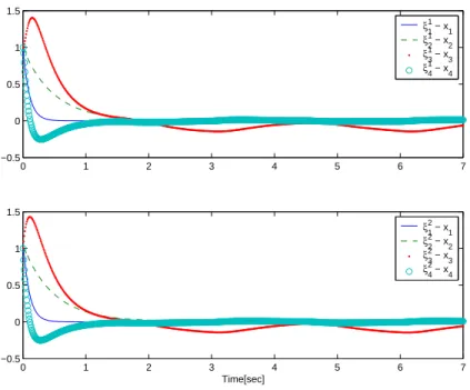
Example 2.1.4 In this case we consider the problem not explicitly addressed in this thesis: we will assume that the system has two deterministic inputs u1 and u2, so that we

have in S (model (4.12)) the additional term    1 0 0 0 0 0 0 1    h_u 1 u₂ i

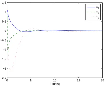
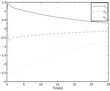
. We take disjoint case as in the Example 2.1.2, and assume that Agent 1 knows only u₁ (square wave), and that Agent 2 knows only u2 (sine wave). The estimator E is applied, with the usual modification taking

care of the locally known deterministic inputs within the local Kalman filters (the consensus scheme remains unaltered) [4].

The given Figures 2.2 and 2.3 represent the estimation errors of ξ1 and ξ2 as functions

of time in the case when k1 = k2= 0 (Fig. 2.2), and in the case when the consensus scheme

exists with k1 = k2 = 10 (Fig. 2.3). It is obvious that the consensus scheme efficiently

reduces the estimation error in spite of the lack of the a priori knowledge about the inputs. 2.1.1.4 Denoising by Consensus

The aim of this subsection is to give an insight into an interesting aspect of the proposed algorithm: its capability to reduce the measurement noise influence as a function of both the number of nodes and the network connectivity. Convergence rate of the schemes for

(24)

0 1 2 3 4 5 6 7 −0.5 0 0.5 1 1.5 ξ₁1_{− x} 1 ξ₂1_{− x} 2 ξ₃1_{− x} 3 ξ₄1_{− x} 4 0 1 2 3 4 5 6 7 −0.5 0 0.5 1 1.5 Time[sec] ξ₁2_{− x} 1 ξ₂2 − x₂ ξ₃2_{− x} 3 ξ₄2_{− x} 4

Figure 2.2: Estimation error for k1= k2 = 10

0 1 2 3 4 5 6 7 0 0.2 0.4 0.6 0.8 1 1.2 1.4 ξ₁1_{− x} 1 ξ₂1_{− x} 2 ξ₃1_{− x} 3 ξ₄1_{− x} 4 0 1 2 3 4 5 6 7 −0.5 0 0.5 1 1.5 Time[sec] ξ₁2_{− x} 1 ξ₂2 − x₂ ξ₃2_{− x} 3 ξ₄2 − x₄

(25)

consensus averaging has been studied in [110, 111]. Pursuing another line of thought, we will analyze asymptotic denoising capabilities of the proposed estimator using simple, yet representative examples of networks with different connectivities.

Case A) Consider first the case when the algorithm E in (2.4) consists of N identical local estimators of the state x of S and a consensus scheme with ˜K = [Kij], Kij = kI, i 6= j,

Kii= −(N − 1)kI, i, j = 1, . . . , N , k > 0 (fully connected graphs). Assuming that wij = 0,

the steady-state estimation error covariance matrix PN satisfies

Φ1P_N+ P_NΦ1T + Q_N = 0, (2.8)

where Φ1 _{= ˜}_{A + ˜}_{K, ˜}_{A = diag { ¯}_{A, . . . , ¯}_{A}, ¯}_{A = A − LC (L is the local steady-state}

optimal Kalman gain), and QN = [QN,ij], QN,ij = ΓQΓT, i 6= j, QN,ii = ΓQΓT +

LRLT, i, j = 1, . . . , N . If T1 =    I I · · · I I −(N − 1)I · · · I · · · I · · · −(N − 1)I    , we have T₁−1KT˜ 1 =

diag{0, −N kI, . . . , −N kI}. Applying T₁−1 and T1 to (2.8), we obtain for N large enough

that the diagonal n × n blocks P_ND,i of PD

N = T1−1PNT1, i = 1, . . . , N become: PND,1≈ N ˆP ,

where ˆP is the solution of the Lyapunov equation ¯

A ˆP + ˆP ¯AT + ΓQΓT = 0, (2.9)

and P_ND,i≈ _2kN1 LRLT_{, i = 2, . . . , N .}

If the average performance index of an estimator is defined as ¯JN = _N1TrPN, we obtain

¯ J_N = 1 NTrP D N ≈ Tr ˆP + 1 2kNTr(LRL T_),

so that ¯J = limN →∞J¯N = Tr ˆP . Obviously, the estimation scheme, averaging different

realizations of the measurement noise, is able to achieve complete asymptotic denoising, since, according to (2.9), the term LRLT is eliminated from the standard local Lyapunov equation

¯

(26)

for the covariance matrix P∗ of one independent local estimator.

Case B) In the case of the consensus matrix with minimal connectivity which still satisfies (A.2.1.2), we have ˜K =

   −kI kI · · · 0 0 −kI kI · · · 0 · · · kI 0 · · · 0 −kI       

N (directed ring). Matrix T2 transforming ˜K to its Jordan form retains from T1 only the first block-column block, so

that P_ND,1 is the same as in Case A). However, we have

( ¯A + λiI)P_ND,i+ P_ND,i( ¯A + λiI)∗+ LRLT = 0, (2.11)

for i = 2, . . . , N , where F∗ _{denotes the conjugate transpose of F and λ}

i are the nonzero

distinct eigenvalues of the consensus matrix (which all lie on a circle with center at (−k, 0) and radius k). According to [78], we have

¯

JN = _N1 TrPN ≥ Tr ˆP + n λmin(LRL T₎

2σmax( ¯A + λiI)

, (2.12)

where λ_min(.) denotes the minimal eigenvalue and σ_max(.) the maximal singular value of an indicated matrix. Consequently, the estimator does not ensure complete asymptotic denois-ing, in spite of the fact that the underlying graph is strongly connected. This conclusion can be readily extended to double directed rings, as well as to all graphs with Laplacians in the form of circulant matrices with a predefined fixed number M of edges entering each node. Namely, in this case we have that maxi|λi| ≤ 2kM , so that the conclusions related

to (2.11) can still be applied (see [28] for properties of circulant matrices). However, the criterion ¯JN still decreases with k. It is interesting that in the simple case of consensus

averaging treated in [110, 111], asymptotic denoising is achieved whenever the underlying undirected graph is connected.

Case C) In general, it appears that the problem of defining the relationship between the network connectivity and the asymptotic denoising achievable by the proposed estimator is difficult. Consider here, however, a special case in which

Tr P_ND,i≤ κi

(27)

where 0 ≤ κi≤ κ < ∞, i = 2, . . . , N . Then, ¯ J ≤ Tr ˆP + lim N →∞ κ (N − 1) N X i=2 1 |λi|. (2.14)

Let 1/|λm1| ≥ . . . ≥ 1/|λmi| ≥ . . . ≥ 1/|λmN|, i = 1, . . . , N . Assuming that for any ε > 0

there exists a positive integer N0 such that 1/|λmi| < ε for all i > N0, we obtain ¯J = Tr ˆP

as in Case A), since the second term in (2.14) tends to zero when N → ∞.

In particular, in the case of Laplacians in the form of circulant matrices treated already in Case B), we have that

λi = k(−M (N ) + M (N )_X

l=1

e−j2πN(i−1)l), (2.15)

i = 2, . . . , N , and that (2.11) holds, where M (N ) represents the number of edges entering each node, which is here supposed to depend on N [28]. It is possible to see that in the case when limN →∞M (N ) = ∞ we have that maxi|λi| = ∞, and that the above

assumption about the nature of the sequence {1/|λmi|} holds, so that, accordingly, (2.14)

implies complete asymptotic denoising.

The given examples show that complete asymptotic denoising results from sufficient graph connectedness.

Communication noise. When the communication noise exists, the Lyapunov equation for the estimation error covariance contains an additional term depending on the matrix Wij = W . Then, for example, one can show that in the case of the fully connected graph

(Case A)) ¯ J = lim N →∞ 1 NTrPN = Tr ˆP1+ k 2TrW. where ¯ A ˆP1+ ˆP1A¯T + ΓQΓT + k2W = 0.

The whole scheme works better than the set of N independent local Kalman filters in spite of the communication noise if Tr ˆP1+k₂TrW < TrP∗, where P∗ is the solution of the Lyapunov

(28)

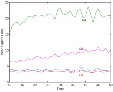
Example 2.1.5 The estimator in this example consists of a set of identical local Kalman filters estimating the whole state of the fourth order system described in Example 2.1.2 (C = I), connected by a consensus scheme. The average criterion ¯J_N = 1

NTrPN has

been calculated as a function of the number of nodes N for the network topologies from Case A) (solid lines) and Case B) (dotted lines); the consensus gain k has been taken as a parameter. The horizontal line corresponds to Tr ˆP , the lower bound obtained by using (2.9). The presented results (Fig. 2.4) fully confirm the given theoretical analysis.

0 10 20 30 40 50 60 70 0.6 0.62 0.64 0.66 0.68 0.7 0.72 0.74 N k=1 k=5 k=50

Figure 2.4: Average criterion as a function of N

2.1.2 Discrete-Time Case

Now, we will consider a discrete-time version of the proposed consensus based estimation scheme, where we will assume that the inter-agent network is lossy, i.e. that communication faults can happen, with some predefined probabilities, and that the local measurements are intermittent.

(29)

2.1.2.1 Problem Definition

Let a finite-dimensional discrete-time stochastic system be represented by

S : x(t + 1) = F x(t) + Ge(t),

y(t) = Hx(t) + v(t) (2.16)

where t is the discrete-time instant, x = (x₁, . . . , x_n)T_{, y = (y}

1, . . . , yp)T, e = (e1, . . . , em)T

and v = (v1, . . . , vp)T are its state, output, input and measurement noise vectors,

respec-tively, while F , G and H are constant n × n, n × m and p × n matrices, respectively. It is assumed that {e(t)} and {v(t)} are white zero-mean sequences of independent vector random variables with covariance matrices Q and R, respectively.

Similarly as in the continuous-time case, we will assume that the i-th agent has a possibility to observe the pi-dimensional vector y(i) = (yli

1, . . . , ylipi)

T_{, composed of the set}

of components of y with indices contained in the agent’s output index set I_iy = {li

1, . . . , lpii},

li

1, . . . , lpii ∈ {1, . . . p}, l

i

1 < . . . < lipi, pi ≤ p. We will assume further that the i-th agent

possesses the local system model S_i defined as

Si: x(i)(t + 1) = F(i)x(i)(t) + G(i)e(t),

y(i)_{(t) = H}(i)_x(i)_{(t) + v}(i)_(t), _(2.17)

i = 1, . . . , N , where x(i) is an ni-dimensional vector composed of the components of x

selected by the agent’s state index set Ix

i = {j1i, . . . , jini}, j i 1, . . . , jnii ∈ {1, . . . n}, j i 1 < . . . < ji ni, ni ≤ n, and v

(i) _{is a measurement noise vector containing the components of v selected}

by I_iy, having the covariance matrix R(i) _{(which can be readily obtained from R); F}(i)_{, G}(i)

and H(i) _{are n}

i× ni, ni× m and pi× ni matrices, respectively.

Starting from the local model Si and the accessible measurements y(i), the i-th agent

is supposed to be able to generate autonomously the local estimate ˆx(i) _{of the vector x}(i)_.

The following local estimator will be assumed to be implementable by the i-th agent: ¯

(30)

where L(i)is the steady state Kalman gain given by L(i) = P(i)H(i)T[H(i)P(i)H(i)T+R(i)]−1, P(i) _{is a solution of the algebraic Riccati equation}

P(i) = F(i)[P(i)− L(i)H(i)P(i)]F(i)T + G(i)QG(i)T, (2.19)

while γ_i(t) is a scalar equal to 1 when the i-th agent receives measurements y(i)_{, and 0}

otherwise ([81]). It is natural to assume that subsystems S_i are defined in such a way that the pairs (F(i)_{, G}(i)_Q1₂_{) are stabilizable and the pairs (F}(i)_{, H}(i)_{) detectable, so that}

the matrices F(i)_{− L}(i)_H(i)_{, the state matrices of the estimators (2.18), are asymptotically}

stable and P(i) _{> 0, i = 1, . . . , N , ([4, 81]). The estimator based on the steady-state gain}

L(i) _{has been selected for the sake of clarity of presentation aimed dominantly at structural}

aspects of the proposed estimator; even better performance can be expected in practice from estimators with time varying gains (see e.g. [81]). In general, the local estimators can be designed using any methodology, in such a way that the general requirements formulated below are satisfied (robust estimators, fault detection filters, etc).

In a similar way as in the continuous-time case, we propose the following algorithm, based on the introduction of a discrete-time consensus scheme:

Ei : ξi(t|t) = ξi(t|t − 1) + γi(t)Li[y(i)(t) − Hiξi(t|t − 1)],

ξi(t + 1|t) =

P_N

j=1Cij(t)Fjξj(t|t) (2.20)

i = 1, . . . , N , where ξ_i is an estimate of x generated by the i-th agent, F_i is an n × n matrix with n_i× n_i nonzero elements that are equal to those of F(i)_{, but are placed at the}

indices defined by Ix

i × Iix, while Hi and Li are pi× n and n × pi matrices, respectively,

obtained from H(i) _{and L}(i) _{in the same way as F}

i is obtained from F(i). We will assume

that Cij(t), i, j = 1, . . . , N , are n × n time-varying gain matrices defining communications

between the nodes, given in the form Cij(t) = kij(t)Kij(t), where kij(t) = 1 when the

directed communication link from the node j to the node i exists, and kij(t) = 0 otherwise;

Kij(t) are diagonal matrices with nonnegative elements, giving appropriate weights to the

(31)

i, j = 1, . . . , N, i 6= j, are mutually independent scalar sequences of independent binary random variables, satisfying P {k_ij(t) = 1} = p_ij and P {k_ij(t) = 0} = 1 − p_ij for i 6= j, as well as that kii(t) = 1, i = 1, . . . , N . Also, we will assume that {γi(t)} is a sequence of

independent binary random variables independent of {kij(t)}, i, j = 1, . . . , N, i 6= j, such

that P {γi(t) = 1} = piiand P {γi(t) = 0} = 1−pii. We will also introduce the random vector

Ξt composed of N2 binary components: N (N − 1) elements kij(t) (i, j = 1, . . . , N, i 6= j)

and N elements γi(t). This vector is, by assumption, generated on the basis of Bernoulli

trials, i.e., {Ξt} represents a sequence of independent random vectors; let πr be the time

invariant probabilities of all possible realizations Ξ[r] of Ξt, r = 1, . . . , ν, ν = 2N 2

.

Define the nN ×nN consensus matrix ˜C(t) = [C_ij(t)], i, j = 1, . . . , N , and assume that it is row-stochastic for all t, i.e. ˜C(t) is a non-negative matrix in which the sum of the elements in each row is equal to one ([30]). This assumption is in accordance with the definition of discrete-time consensus schemes presented in e.g. [39, 72, 107, 57]. Having in mind uncertainty of the communication links, this assumption practically implies recalculation or re-scaling of the sub-matrices Kij(t) composing the consensus matrix ˜C(t) for each new

realization of kij(t), i, j = 1, . . . , N . This re-scaling does not impose any difficulty and can

be easily done locally by each agent in many different ways. One of the straightforward possibilities is to adopt initial diagonal positive semidefinite matrices Kij(0) = Kij0, i, j =

1, . . . , N , according to some predefined criterion (e.g. accuracy of the local estimation), and to obtain ˜C(t) for each t by dividing all the elements of each row of the matrix ˜C0_{(t) =}

[kij(t)K_ij0], i, j = 1, . . . , N , by the sum of all the elements of the same row, i.e. ˜C(t) =

¯c(t) ˜C0_{(t), where ¯c(t) = diag{}P jk1j(t)(K1j0)1, . . . , P jk1j(t)(K1j0 )N, . . . , P jkN j(t)(KN j0 )1,

. . . ,P_jkN j(t)(K_{N j}0 )N}−1and (Kij0)lrepresents the l-th element at the diagonal of the block

K0

ij = diag{(Kij0)1, . . . , (Kij0)N}.

The proposed estimator is strictly scalable as far as the calculation of ξi(t|t) in (2.20) is

concerned, since it does not depend on the number of agents; on the other hand, calculation of ξ_i(t + 1|t) remains scalable as long as each agent communicates with a bounded number of neighbors. Consequently, scalability of the algorithm can be violated only when the structure of the consensus matrix ˜C(t) is such that the number of connections per node tends to infinity when N tends to infinity.

(32)

Let us introduce the following notation: ˜FE= diag{F1, . . . , FN}, ˜Φ = diag{Φ1, . . . , ΦN},

Φ_i = F_i − L_iH_i, and ˜A(t) = ˜C(t) ˜Φ. Introducing ˆX(t|t) = vec{ξ₁(t|t), . . . , ξ_N(t|t)} and ˆ

X(t + 1|t) = vec{ξ1(t + 1|t), . . . , ξN(t + 1|t))}, we can obtain a compact formulation of the

proposed algorithm ˆ

X(t|t) = ˆX(t|t − 1) + ˜L[Y (t) − ˜H ˆX(t|t − 1)] ˆ

X(t + 1|t) = ˜C(t) ˜FEX(t|t),ˆ (2.21)

where Y (t) = vec{y(1)(t), . . . , y(N )(t)}, ˜L = diag{L1, . . . , LN} and ˜H = diag{H1, . . . , HN}

(vec{., .} represents a column vector obtained by concatenation of the column vectors in the braces). Further, for the prediction error ε(t + 1|t) = ˆX(t + 1|t) − X(t + 1), where X(t) = vec{x(t), . . . , x(t)}, we obtain ε(t + 1|t) = ˜A(t)ε(t|t − 1) + ˜C(t)( ˜FE − ˜F )X(t) +

˜

C(t)˜Γ(t) ˜L ˜HV (t) − E(t), where ˜F = diag{F, . . . , F }, V (t) = vec{v(1)_{(t), . . . , v}(N )_{(t)} and}

E(t) = vec{e(t), . . . , e(t)}. Consequently, we obtain the following state space system-estimator model: Z(t + 1) = " ˜ F 0 ˜ C(t)( ˜FE− ˜F ) ˜A(t) # Z(t) + " ˜ G 0 − ˜G ˜C(t) ˜L ˜H # N (t), (2.22)

where Z(t) = vec{X(t), ε(t|t − 1)} and N (t) = vec{E(t), V (t)}. Furthermore, we obtain

¯

Z(t + 1) = ˜B(t) ¯Z(t), (2.23)

where ¯Z(t) = E{Z(t)} and ˜B(t) = " ˜ F 0 ˜ C(t)( ˜FE − ˜F ) ˜A(t) # and

col{P (t + 1)} = ( ˜B(t) ⊗ ˜B(t))col{P (t)} + ( ˜D_[r]⊗ ˜D_[r])col{W }] (2.24)

where P (t) = E{Z(t)Z(t)T_{} and ˜}_{D(t) =}

" ˜ G 0 − ˜G ˜C(t)] ˜L ˜H # and W = E{N (t) N (t)T_{} =} diag{Q∗_{, ˜}_{R}, where Q}∗ ₌    Q · · · Q .. . Q · · · Q  

 and ˜R = diag{R(1)_{, . . . , R}(N )_{}. (col{.} denotes a}

vector obtained by concatenating columns of an indicated matrix and the sign ⊗ denotes the Kronecker’s product).

(33)

2.1.2.2 Stability

In the stability analysis of the proposed estimator, we will use the following results from the matrix analysis.

Lemma 2.1.1 [60] Let f (.) be a matrix norm having the property f (A) ≤ f (B) for two n × n matrices A and B satisfying A ≤ B (A ≥ 0 means that all the elements of A are nonnegative). Let g(.) be any matrix norm and let A be partitioned into square blocks Aii.

Then, h(A) is a matrix norm, where

h(A) = f       g(A11) · · · g(A1k) .. . ... g(Ak1) · · · g(Akk)       . (2.25)

Lemma 2.1.2 ([30], Lemma 5.6.10) Let A be an n × n matrix and ε > 0. Then, there exists a matrix norm kAk such that

ρ(A) ≤ kAk ≤ ρ(A) + ε, (2.26)

where ρ(A) is the spectral radius of a matrix A (ρ(A) = maxi|λi(A)|, where λi(A) are the

eigenvalues of A).

A norm satisfying the requirement (2.26) is the norm kAkτ = kDτUTAU Dτ−1k∞,

where U is an orthogonal matrix in the representation A = U ∆UT_{, where ∆ is an}

up-per triangular matrix (according to the Schur’s theorem), Dτ = diag{τ, τ2, τ3, . . . , τn} and

kAk∞= maxi

P_n

j=1|aij| (for A = [aij], i, j = 1, . . . , n). Inequality (2.26) is satisfied for any

given ε > 0 by choosing τ ≥ 0 large enough.

The following two theorems give sufficient conditions for stability of the proposed algo-rithm in the sense of convergence to zero of the estimation error mean and boundedness of the mean-square error. The analysis is based on the definition of a new, specially con-structed norm according to Lemma 2.1.1, adapted to the partition of the consensus matrix

˜

C(t) into the blocks Cij(t), and the methodology from [81, 54, 55].

(34)

are realizations of Cjk(t) and Φj(t) obtained by choosing Ξt= Ξ[r], and let ρ(Φ[r]_k ) < b[r]_k < ∞, k = 1, . . . , N , together with ν X r=1 πrmax j N X k=1 ρ(C_jk[r])b[r]_k < 1. (2.27)

Then, limt→∞E{ε(t|t − 1)} = 0 if the system (2.16) is asymptotically stable. If the system

(2.16) is not asymptotically stable, limt→∞E{ε(t|t − 1)} = 0 if, additionally, ˜FE = ˜F .

Proof: Consider the matrix ˜A_[r] and define its norm k ˜A_[r]k? in the following way:

k ˜A_[r]k? = ° ° ° ° ° ° ° ° °      kC₁₁[r]Φ[r]₁ kτ · · · kC_1N[r]Φ[r]_Nkτ .. . ... kC_{N 1}[r]Φ[r]₁ k_τ · · · kC_{N N}[r] Φ[r]_Nk_τ      ° ° ° ° ° ° ° ° ° ∞ , (2.28)

having in mind properties of the norm k.k∞, and Lemma 2.1.1. For particular terms in

(2.28) we have that kC_jk[r]Φ[r]_k kτ ≤ ρ(C_jk[r])kΦ[r]_k kτ, having in mind that kC_jk[r]kτ = ρ(C_jk[r]) for

diagonal matrices C_jk[r]. Moreover, it is always possible to find such a ¯τ > 0 that for any τ > ¯τ we have kΦ[r]_k k_τ ≤ ρ(Φ[r]_k ) + ε, for any given ε > 0. Making ε small enough we always have that ρ(Φ[r]_k ) + ε ≤ b[r]_k (having in mind that the assumption ρ(Φ[r]_k ) < b[r]_k is in the form of a strict inequality). Therefore, kΦ[r]_k kτ ≤ b[r]_k , and consequently,

k ˜A_[r]k? ≤ max j N X k=1 ρ(C_jk[r])b[r]_k ,

so that the matrix Pν_r=1πrA˜[r] is Hurwitz if (2.27) holds, implying that the model for the

mean (2.23) is asymptotically stable if ˜F is Hurwitz. The second statement of the Theorem follows trivially from the definition of the matrix ˜B_[r], since E{X(t)} and E{ε(t|t − 1)} become decoupled. Thus the result.

Theorem 2.1.3 The proposed estimator provides kS(t)k < ∞, where S(t) = E{ε(t|t − 1)ε(t|t − 1)T_{}, ∀t ∈ I, (I is the set of all integers), if ρ(Φ}[r]

k ) < b [r] k < ∞, k = 1, . . . , N , ν X r=1 πr[max j N X k=1 ρ(C_jk[r])b[r]_k ]2 < 1 (2.29)