Marcos Octávio da Silva Estrela
Licenciado em Ciências da Engenharia Eletrotécnica e de Computadores
DC Traction system cost estimation tool taking
into account losses minimization
Dissertação para obtenção do Grau de Mestre em Engenharia Electrotécnica e de Computadores
Orientador: Professor Doutor João Martins, Professor Associado, Universidade Nova de Lisboa
Júri
Presidente: Professor Doutor Luis Oliveira Vogais: Professor Doutor João Murta Pina
Copyright © Marcos Octávio da Silva Estrela, Faculdade de Ciências e Tecnologia, Univer-sidade NOVA de Lisboa.
A Faculdade de Ciências e Tecnologia e a Universidade NOVA de Lisboa têm o direito, perpétuo e sem limites geográficos, de arquivar e publicar esta dissertação através de exemplares impressos reproduzidos em papel ou de forma digital, ou por qualquer outro meio conhecido ou que venha a ser inventado, e de a divulgar através de repositórios científicos e de admitir a sua cópia e distribuição com objetivos educacionais ou de inves-tigação, não comerciais, desde que seja dado crédito ao autor e editor.
Este documento foi gerado utilizando o processador (pdf)LATEX, com base no template “novathesis” [1] desenvolvido no Dep. Informática da FCT-NOVA [2].
Ac k n o w l e d g e m e n t s
I would like to express my gratitude to all that allowed me to achieve this objective in my life, it represents an end of a succeeded journey.
Firstly, I would like to thank my advisor Professor João Martins, for the opportunity, knowledge and for believed me to develop this dissertation.
A profound acknowledgment to my family and girlfriend for the strength and uncon-ditional support provided along these years. I owe you this thesis for having taught me to believe that with effort everything can be achieved and giving up is not a solution.
I wish to thank to all in Efacec, where I worked while developing this dissertation, whose share me knowledge and support me to develop this work. A special thanks to Eng. Miguel Leão for all the knowledge and consistently feedback provided during this process.
My journey through this university is finishing, so, many thanks to Faculdade de Ciências e Tecnologias of Universidade Nova de Lisboa for the opportunity to enlarge my knowledge and to allow met all the people during these years. Also thanks for all the challenges, it allowed me to grow and being the person I am today.
Finally, to all my friends who where part of this journey, that provide me continuous encouragement throughout my years of study and for all the good moments spent during this time. Thank you.
A b s t r a c t
This dissertation proposes a tool that will give support to the design of DC traction systems. The tool simulates a simplified model, with three substations and the goal is to find the system configuration that minimizes the distribution system (catenary) losses.
The existing software tools allow to simulate power traction systems, although, it is usual to take long time to optimize them and carries difficulties to find optimal solutions. The tool presented in this work, developed in a simulation software, allows modeling a system, where a vehicle operates in a line, fed by a traction supply system composed by three traction substations. It becomes possible to simulate the system, considering all the assumptions and simplifications, getting mechanical and electrical results. The methodology allows to size the traction groups, the section for parallel feeder cable and the length of each electrical section, using the best location for the intermediate substa-tion.
A comparative study between two scenarios is proposed and it is presented a method to globally simulate the system, verifying the best configuration between the several hy-pothesis. Thus giving the best solution for the system in analysis.
R e s u m o
Esta dissertação propõe uma ferramenta que dará suporte aos estudos de tração ali-mentados a corrente continua. O algoritmo desta ferramenta simula um modelo sim-plificado com três subestações e o objetivo é encontrar a configuração de sistema que minimiza as perdas no sistema de distribuição (catenária).
As ferramentas existentes permitem simular sistemas de tração de potência, apesar de, usualmente ser um processo demoroso e que apresenta dificuldades para encontrar soluções ótimas.
A ferramenta apresentada nesta dissertação, desenvolvida com um software de si-mulação, permite modelar um sistema, onde um veiculo opera ao longo de um troço de via, alimentado por três subestações de tração. Considerando todas as simplificações inerentes ao desenvolvimento, permite a possibilidade de simular o modelo, extraindo resultados mecânicos e eléctricos da operação. A metodologia permite dimensionar os grupos retificadores das subestações, a secção do cabo paralelo de tração, bem como o comprimento das secções elétricas, através da posição ótima da subestação intermédia.
Um estudo comparativo entre dois cenários é proposto e é apresentado um método para globalmente simular o sistema, verificando a melhor configuração entre as várias hipóteses. Portanto, dando a melhor solução para o sistema em análise.
Palavras-chave: modelação, tração, energia, transportes, optimização, Simulink®, Ma-tlab®.
C o n t e n t s
List of Figures xiii
List of Tables xvii
Acronyms xix 1 Introduction 1 1.1 Motivation . . . 1 1.2 Objectives . . . 3 1.3 Dissertation Structure. . . 4 2 State-of-the-Art 5 2.1 Introduction . . . 5
2.1.1 Physical parameters of a system . . . 6
2.1.2 Track gradient . . . 8
2.1.3 Train Mass . . . 9
2.1.4 Maximum Acceleration and Braking . . . 9
2.1.5 Regenerative braking . . . 10
2.1.6 Location of the power substations . . . 11
2.2 Existing Simulating tools . . . 11
2.2.1 Existing simulating tools . . . 13
2.2.2 Projects designed by software simulators. . . 16
2.3 Genetic Algorithms . . . 17
3 Proposed design methodology 19 3.1 Model . . . 20
3.1.1 General synthesis methodology . . . 26
3.1.2 Dynamic variables modelling . . . 34
3.1.3 Electrical system modelling . . . 35
3.2 Financial evaluation . . . 40
3.3 GA Method . . . 41
3.3.1 Genetic algorithm . . . 41
4.1 Resume of the cases studies . . . 43
4.1.1 Case Study input data . . . 44
4.1.2 Results from the simulation . . . 49
4.1.3 Case Study 1: [PFC120]. . . 53
4.1.4 Case Study 2: [PFC400]. . . 64
4.1.5 Case Study comparative analysis . . . 69
4.1.6 Cost estimation using Matrix Method - Global Finder Simulation. 71 4.1.7 Cost estimation using GA Method . . . 80
5 Conclusions and Future Work 81 5.1 General Conclusions . . . 81
5.2 Future Work . . . 82
L i s t o f F i g u r e s
1.1 Tram Citadis 401 in Bernburb Street of Dublin. . . 2
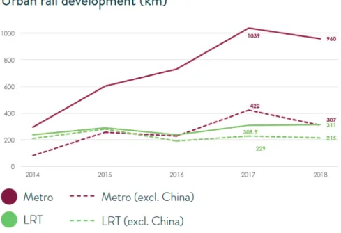
1.2 Urban Rail development in km for Metro and Light Rail Transportation rail (LRT) systems . . . 2
1.3 Vehicle operating in a 750Vdc traction system, adapted from [11]. . . 3
2.1 DC traction system general structure, adapted from [11]. . . 5
2.2 Overhead contact system and rails circuit . . . 6
2.3 Yizhuang line map from Beijing metro system, from [6]. . . 7
2.4 Timetable graphic representation, adapted from [20]. . . 8
2.5 Load Power along a sloping route . . . 9
2.6 Immediate energy exchange between trains by regenerative braking, from [29]. 10 2.7 Process during the operation simulation . . . 12
2.8 Trainsrunner design interface, from [23] . . . 14
2.9 eTrax design interface, from [28] . . . 14
2.10 Flowchart of GA System, adapted from [12]. . . 18
3.1 High Level Simulation process flow . . . 20
3.2 DC traction system considered . . . 21
3.3 Representation of the interface between Excel and the simulation software . 21 3.4 S200 high floor light rail vehicle, from [25]. . . 22
3.5 Simulink blocks used to model the speed control system using a PID . . . 23
3.6 Example of the speed control results . . . 24
3.7 Headway between two vehicles. Adapted from [14] . . . 24
3.8 High level simulink model representation . . . 25
3.9 Optimized variables used in simulation, (LOC and PFC).. . . 26
3.10 Example of consumption profile from three substations located consecutively in a track . . . 27
3.11 Substation single line diagram . . . 28
3.12 DC traction system . . . 29
3.13 Representation of possible TPS2 locations in percentage value of the total length of the route . . . 30
3.14 Inside overview of a typical traction power substation [Adapted from Siemens] 32 3.15 Typical Electrification of railway [Adapted from [26]] . . . 32
3.16 Cross section of a feeder underground cable . . . 33
3.17 Example of a Traction Transformer, from Efacec Power Solutions Linkdin page. 33 3.18 Typical traction and braking effort curves . . . 34
3.19 First electrical section circuit modelled in simulink . . . 36
3.20 Second electrical section circuit modelled in simulink . . . 36
3.21 Electrical schematic model . . . 37
3.22 Example of power diagram from three substations . . . 38
4.1 Image of the inserted speed profile . . . 44
4.2 Traction Effort limitation curve from the vehicle . . . 47
4.3 Speed limits and Speed performed by the vehicle . . . 49
4.4 Position performed by the vehicle . . . 50
4.5 Acceleration performed by the vehicle . . . 50
4.6 Power required by the vehicle along the track . . . 51
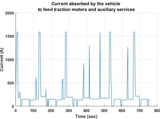
4.7 Current required by the vehicle used to feed traction motors and auxiliary services . . . 52
4.8 Impact of the variation of TPS2 on the drop voltage in contact line . . . 53
4.9 SC1: Substations Power Diagram locating TPS2 at 30% of the route . . . 54
4.10 SC1: Substations Power Diagram locating TPS2 at 40% of the route . . . 55
4.11 SC1: Substations Power Diagram locating TPS2 at 80% of the route . . . 55
4.12 Energy consumption by TPS1 along the track . . . 56
4.13 Energy consumption by TPS2 along the track . . . 57
4.14 Energy consumption by TPS3 along the track . . . 57
4.15 Current delivered by substations using a 120sq. mm cable as feeder cable and locating TPS2 at 30% of the route . . . 58
4.16 Current delivered by substations using a 120sq. mm cable as feeder cable and locating TPS2 at 80% of the route . . . 59
4.17 Catenary losses using a 120sq. mm cable as feeder cable and locating TPS2 at 30% of the route . . . 60
4.18 Catenary losses using a 120sq. mm cable as feeder cable and locating TPS2 at 40% of the route . . . 60
4.19 Catenary losses using a 120sq. mm cable as feeder cable and locating TPS2 at 80% of the route . . . 61
4.20 SC1: 3rd configuration - First electrical section contact wire current flow . . 62
4.21 Study case 1: Investment cost and estimated losses along the time . . . 62
4.22 SC2: Impact of the variation of TPS2 on the drop voltage in contact line . . . 64
4.23 Current delivered by substations using 400sq. mm cable as feeder cable and locating TPS2 at 30% of the route . . . 65
4.24 Current delivered by substations using 400sq. mm cable as feeder cable and locating TPS2 at 40% of the route . . . 66
L i s t o f F i g u r e s
4.25 Current delivered by substations using 400sq. mm cable as feeder cable and
locating TPS2 at 80% of the route . . . 66
4.26 SC1: 3rd configuration - First electrical section contact wire current flow . . 67
4.27 Study case 2: Investment in cable and estimated losses cost along 25 years of operation . . . 68
4.28 Case studies 1 and 2: Impact of using different configurations on catenary losses along 25 years operation. . . 69
4.29 Study case 1 and 2: Investment cost, estimation losses cost and the relative best solution . . . 70
4.30 Surface graph that shows the impact of the variables variation on the estimated losses . . . 72
4.31 Achieved best configuration overview. . . 73
4.32 Route map overview . . . 73
4.33 Best configuration: Contact wire drop voltage . . . 74
4.34 Best configuration: Substations Power diagram . . . 74
4.35 Current delivered by substations using 240sq. mm cable as feeder cable and locating TPS2 at 40% of the route. . . 75
4.36 Catenary Losses using the achieved best configuration . . . 76
4.37 Achieved optimal solution estimative cost evolution: Investment feeder cable and catenary losses . . . 77
4.38 Comparison estimative cost evolution: Investment feeder cable and catenary losses . . . 78
L i s t o f Ta b l e s
2.1 Usual input data used by existing simulator tools . . . 12
2.2 Main Features of existing simulator tools . . . 15
3.1 Two-way table that represents the sample space relatively the system configu-rations . . . 26
3.2 Parallel feeder cable used in the software tool . . . 30
3.3 Substation Equipments considered and respective unitary prices . . . 31
3.4 Considered cables and respective unitary prices . . . 31
3.5 Tariff for sale to final customers in MV [Translated from ERSE, 2018b] . . . . 40
3.6 Parameters bounds used in function @ga . . . 41
4.1 Input speed profile . . . 45
4.2 Stations considered in simulation . . . 45
4.3 Vehicle considered in simulation . . . 46
4.4 Traction Effort . . . 46
4.5 Operation modes input data . . . 47
4.6 Potential locations for substation TPS2 according the lenght of the route. . . 48
4.7 Configuration considered in the Case Study 1 . . . 53
4.8 Individual and total energy consumption for each configuration . . . 56
4.9 Estimated Catenary losses and respective cost . . . 59
4.10 Configuration considered in the case study 2 . . . 64
4.11 Individual and total energy consumption for each configuration . . . 65
4.12 Catenary Losses and respective estimated cost for 25 years of operation . . . 65
4.13 Best relative solution detailed cost. . . 70
4.14 Best configuration for 25 years operation . . . 73
4.15 Substations Consumptions . . . 75
4.16 Resulted Losses . . . 76
4.17 Best configuration parameters final costs . . . 79
Ac r o n y m s
AC Direct Current.
D12 Distance between substations TPS1 and TPS2. D23 Distance between substations TPS2 and TPS3. DC Direct Current.
GA Genetic Algorithm.
LOC Substation TPS2 location code reference. LRT Light Rail Transit.
PFC Section of Parallel Feeder Cable code reference. PID Proportional-Integral-Derivative.
PK Point Kilometric.
RMS Root Mean Square.
ST Station.
C
h
a
p
t
e
r
1
I n t r o d u c t i o n
1.1
Motivation
The current outlook of the world relatively the high consumption of fossil fuels and the warn of the decrease in the amount of reserves, becomes fundamental to optimize as most as possible the transportation railway systems and avoid losses.
This dissertation offers a complementary tool to study and understand a DC traction system.
The software tool of this dissertation offers not only a complementary tool to existing simulator tools, but also an opportunity to study and understand a DC traction system. The possibility of identifying possible optimal solutions for a traction system, in par-ticular through an economic analysis of its operation is the main motivation for this dissertation.
This type of systems has many advantages, such being relatively eco-friendly, easier to handle, that allows easy speed control, high efficiency and low maintenance.
DC traction systems usually use light rails or trams, as their rolling stock, to operate the lines. As example, in figure1.1can be seen the tram operating in Dublin city [8]. To feed these vehicles a power supply system is used, which is the main scope of this dissertation. These systems are considered convenient, sustainable and environmentally friendly. Higher prices for energy resources and the growing number of passengers that are shifting away from private transport to public transportation shows that it is becoming increasingly important to optimize these systems [1].
2018 was a successful year for urban rail infrastructure, despite a 6% slowdown of growth pace. 121 urban rail projects were completed on all continents, totaling 1270 km, com-pared to 1348 km in the previous year. It is registered that, 75 individual metro infras-tructures projects were completed in 39 cities, in a total of 960 km. For Light rail market,
it is registered that 46 single infrastructure projects were completed in 40 cities, in a total of 309 km [31]. These numbers are presented in figure1.2.
This dissertation proposes the development of a methodology that allows to optimize a DC traction system, as to the position of the middle substation and the section for the parallel feeder cable.
Figure 1.1: Tram Citadis 401 in Bernburb Street of Dublin.
Figure 1.2: Urban Rail development in km for Metro and Light Rail Transportation rail (LRT) systems
1 . 2 . O B J E C T I V E S
1.2
Objectives
This dissertation will focus on an automated software tool that allows to estimate the minimum cost for a DC traction system (estimated energy supply system and losses costs). The first objective is to create an automated process that allows achieving the optimum system configuration. To find this optimum configuration, the process will have to simulate an operation condition and extract electromechanical results. In figure
1.3is possible to see a scheme that shows a vehicle operating in a 750 Vdc traction system, which uses an energy distribution system and two common traction substations. The second objective is to identify and evaluate the situations where it is profitable to use a higher section for parallel feeder cable. Using a higher section will lead a decrease of losses in the catenary circuit, for the same operation conditions.
Figure 1.3: Vehicle operating in a 750Vdc traction system, adapted from [11].
In resume the thesis objectives are:
• Develop a DC traction system model that allows to simulate an operation with one vehicle and three substations and extract the respective electromechanical results.
• Develop a methodology to use the simulation results, from first point, and estimate the best system configuration taking into account losses minimization;
• Elaborate a comparative analysis that shows the system configuration impact on catenary losses.
1.3
Dissertation Structure
This dissertation is divided in five chapters. The first chapter is an introduction to the project, explaining and justifying the purpose of this dissertation and detailing the respective structure.
The second chapter introduces the main characteristics about DC traction systems using relevant published literature. Then is presented some railway simulator tools, describing their methodology and showing their features.
The electric traction system model and the calculation methods is shown in third chapter, including reference values for traction supply equipment.
In chapter four is showed the simulation results in order to analyses and evaluate the used calculation model. It is showed a comparative study between system configurations, evaluating the best configuration.
For last, in chapter five is presented the final conclusions of this dissertation and it is showed the suggestions for a future work.
C
h
a
p
t
e
r
2
S ta t e - o f -t h e -A rt
This chapter presents the conclusions from published research literature and present the most used railway simulator tools.
2.1
Introduction
This section shows some research that has been published in the recent years. To get a sustainable urban rail transportation, each detail has to be taken into account during the traction system design.
The DC traction power system is composed of the consumers, which is mainly the vehicles that operate in the track, and the power supply system, composed of: substations and the distribution system (catenary), as shown in figure2.1.
In the DC traction system of urban rail transportation, substations are the facilities that provides the 750V or 1500V voltage for the vehicles to run and they are placed along the route spaced, usually, between one and three, for 750V and between three and six, for 1500V [11].
The traction distribution system is mainly composed of the catenary circuit and rails circuit. The catenary system is composed of a contact wire and usually by a parallel feeder cable, that allows for provide a higher current flow to fed the vehicles. The conductor material, are usually copper or aluminum. Figure2.2shows a catenary and rails systems.
Figure 2.2: Overhead contact system and rails circuit
2.1.1 Physical parameters of a system
Physical parameters that influence the traction system performance have been ex-plored and are presented below. The performance are evaluated by the operation effi-ciency, considering mainly by the trip time and the consumption.
• Operation schedule and timetable. These parameters define the exploration ca-pacity of the line;
• Track gradient. Positive and negative slopes of the track;
• Vehicle mass. Representing the vehicle tare plus the respective capacity during an operation;
• Limitation on acceleration and deceleration values. Fundamental parameter from vehicle kinematics, that might influence directly the operation consumption.
2 . 1 . I N T R O D U C T I O N
• Regenerative braking. It is an energy recovery mechanism that allows the vehicles that are braking to generate electricity back to distribution system and being used by other vehicles, saving energy from the power source;
• Traction Power Substations locations.
To show the importance of these parameters it was explored a report made in 2016, where some simulation results was achieved using real data from Beijing Yizhuang line, which belongs to Beijing metro system, in China. The line has around 23 km of railway. It started operating in 2010 and it has 14 stations, including six underground, to ensure the daily transportation of 173.5 thousand passengers in average, values from 2014 [6] [30].
Figure 2.3: Yizhuang line map from Beijing metro system, from [6].
According to this study, the possible factors that influence the traction energy con-sumption are the trip time, the track gradient, the running resistance, the maximum traction and braking forces, the regenerative braking and the train mass, as can be seen as follow [29].
2.1.1.1 Operation schedule and timetable
Increasing the trip time, the energy consumption decreases. As an example is showed that the consumption increases by 3.4 kWh when the trip time is reduced from 160 to 150 seconds, compared to 4.8 kWh when the trip time is reduced from 150 to 140 seconds. So, two techniques can be applied, as can be seen below:
• Increase the trip time by reducing the time where the train is stopped;
• Timetable optimization.
A timetable from a public transport service is a document that shows the information of the schedules during specific hours of the day, it allows to assist passengers with a planning trip.
It can be represented as a Position/Time graphic that shows the vehicles trajectory during the time trip, as can be seen in figure2.4.
The main purpose to use timetables information in simulation designs are to achieve the best possible exploration capacity by using the railway infrastructure [21].
Figure 2.4: Timetable graphic representation, adapted from [20].
Other authors developed techniques to optimize the timetable: Lin Chen, suggests to apply genetic algorithms to optimize train scheduling. The main idea is to avoid the simultaneous acceleration from many trains, in order to reduce the maximum traction power [5].
2.1.2 Track gradient
In the region where the vehicle climbs up the consumption tends to increase, which increases the voltage drop on contact line, from the supply network distribution. This impact was studied by Nguyen Viet [19]. In figure2.5, it is possible to see the referred situation representation.
The authors from [29], also studied the track gradient impact on the vehicle’s energy consumption. Psychically, it occurs because more traction force must be applied to deliver the required trip time for a steeper uphill climb. The results shows that the consumption increases 0.8 kWh when the gradient of the starting section gains 0.2% uphill, compared to only 0.1 kWh for the middle and caudal sections [29].
2 . 1 . I N T R O D U C T I O N
Figure 2.5: Load Power along a sloping route
little influence on the total traction energy consumption of the operational systems, al-though the slopes near stations could contribute to saving energy. For trains running in the middle section, the downhill slope could help the trains achieve a high speed in a shorter time [29]. For these reasons, important measures of the energy-efficient gradient design are concluded as follows.
• Increase the gradient near stations;
• Proper length of the gradient.
2.1.3 Train Mass
The influence of the train mass on the traction energy consumption was studied in [29]. To see this influence, the running time has being fixed. It was cleared verified that the heavier the train is, more energy it will be used during the trip. The results show that the energy consumption is nearly doubled when the train mass increases by 50%. Hence, a mass reduction is proposed as one of the important strategies to save energy, mainly by developing vehicle structures with lighter materials, such as aluminum or alloy [29] [4].
2.1.4 Maximum Acceleration and Braking
The acceleration and braking maximum values are usually choose by the estimated passenger comfort level. However, this value might affect hugely the operation consump-tion [21].
Typically these values are between 0.02 and 1 m/s2for heavy trains and 1 and 3 m/s2for metro and light transportation systems.
The results reveal that the consumption has a gentle decrease with the increase of the maximum traction and braking forces. Numerically, these consumptions are 23.9, 23.5, 22.5 and 21.9 kWh, with the corresponding maximum braking forces 255, 270, 305 and 345 kN. Comparing with two different speed profiles, it was discovered that the train with a higher braking rate can come to a stop more quickly, and therefore a lower speed is needed to perform the operation and complete the route, which could reduce the global
consumption in the operation. In conclusion, vehicles with larger limitation to traction and braking forces are more efficient [29].
2.1.5 Regenerative braking
An efficient use of the regenerative energy could make a great difference in reducing the energy consumption in systems. The energy is fed back to the power network, such that it can be used by other accelerating trains. The energy could also be stored in storage systems and be reused by trains later.
For the storage of the regenerative energy, batteries, super-capacitors or fly wheels, should be installed. These storage systems can be divided into two types, on the trains or along the track side. The on board systems, can only be used by the train which sup-ports it. The advantage is the increase of the efficiency. However, on board installations will increase the vehicle’s weight. On the other hand, the wayside systems, can store the regenerated energy when nearby trains are applying regenerative braking. For this reason, it is important that these systems are installed near stations, so the stored energy can be reused by other trains. The main advantage is the possibility to recover from multiple braking trains at the same time, however, these solutions are less efficient due the transmission losses on the power line [29] [7].
Figure 2.6: Immediate energy exchange between trains by regenerative braking, from [29].
So, this concept, working without storage equipment, as shown in figure2.6, have some constraints, when a train is braking on the track, the other train should be in accel-eration, in the other track, at the same moment. If there is no train in traction movement to receive the energy from a braking train, this energy is wasted, by a proper dissipation to earth [29].
With the very frequent starting and stopping of trains, it was found that 53% of the total energy consumption will be released during the braking stage. By subtracting the loss of motion resistance and mechanical braking, there is 22% of the energy consumption that can be restored by electric regeneration. These values occur only if the rectifiers are installed at proper locations along the line [7].
2 . 2 . E X I S T I N G S I M U L AT I N G T O O L S
In conclusion, the trains should be matched in the proper timing and in space. In other words, the strategies are [7] [29]:
• the optimization of the train timetable;
• rectifier substations installed at proper locations;
• storage systems installed near stations.
2.1.6 Location of the power substations
An easy method to locate substations is to place them near the stations because it is where the power demand is high. However, civil constraints might be a problem.
Study optimization techniques for substation placement for DC traction systems have been developed along the years, and it is extremely important to apply those techniques or improve them.
Some research papers had the objective to optimize these placements. As previously mentioned, the author from [7] suggests placing the substations optimally for an accurate energy regeneration. The author from [19], suggests an algorithm to optimize a traction system for personal rapid transit, with the objective to minimize the energy losses on the network. This method locates the power supplies optimally for load balancing and uses an iterative approach based on thevirtual isolation concept between substations. Basically, the optimal location of the substations is according to the geometric environments and the load power, in order to minimize it power rating. Although, this method doesn’t consider some electrical requirements, regarding for example, the maximum drop voltage in the contact line.
2.2
Existing Simulating tools
The advantage to simulate electrical traction systems is the support to study and eval-uate the best electrical configuration for a system, comparing different scenarios.
The simulators take into account the vehicle movement characteristics and the elec-trical power supply behavior in each instant.
The aspects that affects a supply system behavior are the interactions between the rolling stock, the route, the substations and other equipments. These informations provide a large amount of data and complicated calculations must be done by the software simula-tor tools [21].
The figure2.7shows a schematic that represents the process design simulate a system. Modeling a railway system requires two sequenced calculations, the mechanical and then the electromechanical. Simulating a mechanical system, means calculating the train
Figure 2.7: Process during the operation simulation
motion along the track, using ideal electrical conditions, without losses and considering that there is no drop voltage in contact line. It allows the user to decide properly the simulation time to use in the complete electromechanical simulation. In this last, it is needed more time to simulate, because means solving the power flow by considering all the inputs. So, optimize the simulation time is fundamental to save time during an optimization process.
Also, to use the right data from the vehicle, the general software tools allow full spec-ifications to be inserted, which represents the system load representation.
The general parameters, used in the simulators, are indicated in table2.1.
Table 2.1: Usual input data used by existing simulator tools
Track Vehicle Electrical
Stations Weight
Traction
transformer
Curves Traction and braking effort
Positive line resistance
Slopes Maximum speed Negative line resistance
Speed limits Auxiliary
consumptions Energy storage Tunnels Regenative braking Shunt connectors
The tool developed in this dissertation allows the user to insert some of these inputs, mentioned in table2.1, such as regarding the track: stations, slopes and speed limits. All the inputs regarding the vehicle, refereed in table, can be inserted, unless the regenera-tive braking. Regarding electrical data, is possible to introduce almost all of these inputs, considering the simplifications, such as, only is possible to consider one shunt at middle distance between the positive network from electrical sections and the power supply uses
2 . 2 . E X I S T I N G S I M U L AT I N G T O O L S
an ideal voltage source. Energy storage are not considered in the electrical model of this software tool.
The software tool of this dissertation unlike others, optimize automatically the trac-tion system, giving it the best substatrac-tions’ tractrac-tion group nominal power values, the parallel feeder cable cross section area and the position of the intermediate substation.
2.2.1 Existing simulating tools
Generally, the existing simulators can perform realistic electro-mechanical simula-tions for AC/DC railways, inclusive light rails, metros or trolleybus systems. Usually, they provide the analysis of system performances and their consumptions.
Below are stated the current commercially available software tools and they are mostly used by traction systems engineers.
• TrainsRunner, by Setteidea Srl, from [24];
• OpenTrack and Open Power Net, by Technical university of Zurich, from [20];
• TrainOp, by LTK Engineering Services, from [16];
• Sitras Sidytrac, from [27];
• EtraX, from [10].
The essential features of these softwares that allow the development of the traction model accurately, are the user-friendly graphical interface, simulating signaling systems, evaluation consumptions, simulate failures conditions, etc. Figures 2.8 and2.9 show graphical interfaces that allow the user an overall graphic visualization of the system.
The signaling systems are useful tools, because allow simulating eventual train stops, that usually potentially lead to higher consumption levels during an operation.
On other hand, there are some limitations associated to these softwares such as the lack of automatic solvers to optimize the systems. So the users iteratively optimize the systems by consecutive electromechanical simulations. Also it is not usual, simulators consider an integrated economical solver, that theoretically would helps the users to study the configuration system impact on the solution costs. Also, it is not usual these tools to support simulate the medium voltage network in order to study the influence on the DC traction system.
Figure 2.8: Trainsrunner design interface, from [23]
2 . 2 . E X I S T I N G S I M U L AT I N G T O O L S
Table2.2shows the main features and the constraints, of these existing software tools.
Table 2.2: Main Features of existing simulator tools
Simulators/
Features eTraX OpenPower
Trains Runner Sitras Sidytrac TrainOp Evaluate consumptions 3 3 3 3 3 Evaluate equipment losses 3 3 3 3 3 Regenerative braking 3 3 3 3 3 Harmonics results 3 3 3 3 3 EMC results 3 3 3 3 3 Automatically generates optimal power configurations 7 7 7 7 7 Automatically generates the optimal eletrical sections lenghts
7 7 7 7 7
Automaticaly generates the best configuration taking losses into account
2.2.2 Projects designed by software simulators
In this section are presented two recent railway projects, where it was been used sim-ulating tools.
In 2015, LTK Australia using the simulator TrainOps, simulated and studied the Mel-bourne tram railway, in Australia. The main goal was to report the issues and generate potential traction power upgrades to accommodate 110 new E-Class trams. These tram railway system are considered to be the longest in the world, with 250 km of double tracks, with 24 routes, 1679 passenger stops and a fleet of nearly 500 vehicles. After identifying 33 potential traction power upgrades, including new substations TrainOps was used to quantify the criticality of each potential upgrade. This study allowed decision makers to confirm the minimal requirements to introduce the new, more power demanding trams [15].
In 2017, TrainsRunner was used to simulate the Odense Light Rail, in Denmark. This system has 14 km of line, 26 stations and 14 vehicles to operate in the line. The DC supply system is composed by eight traction substations, located along the line. It is expected this system will carry 34 thousand passengers daily and is planned to be operational by the end of 2020 [9].
2 . 3 . G E N E T I C A L G O R I T H M S
2.3
Genetic Algorithms
Software simulator tools usually don’t have as a feature the application of genetic algorithms, although this dissertation looks to apply genetic algorithms as a method to solve optimize the systems configurations, finding optimal solutions.
Genetic algorithm are based on natural evolution, appreciated as a simple and con-sistent mechanism, that can be used to optimize models. Independent of the initial conditions of the algorithm, it generates high quality results, the reason why this mecha-nism is considered as consistent.
The genetic algorithm’ main focus is the creation of descendants using recombination operators. Besides that, the mixed use of the mutation operators recombinations allows for the balance of two apparently conflicting goals: The best solutions harnessing and the search space of exploration. Thus, the genetic algorithms find the optimum point based in a candidates solutions population, and not just using a single point, using probabilistic transition rules [18] [12].
In figure2.10can be seen the flowchart regarding a classic genetic algorithm. The traditional AG follows the following steps:
1. The initial population of chromosomes is generated by an aleatory process;
2. The population is evaluated according to its fitness, where each chromosome re-ceives a value, which reflects its quality relatively to the problem’s solution;
3. Chromosomes are modified by genetic operators, with the purpose to modify the population;
4. Then is created a new generation, taking the previous step into account ;
5. Steps 2 and 4 go in loop, until the satisfied solution has been reached.
Applying GA in optimization problems has been largely used, although it is important to correctly define the input parameters, which depends on the specific problem to be handle. The following list shows these parameters [12]:
• Population: The population size affects directly the GA global performance and effectiveness. The population with few individuals leads to a small search cover, which lowers the performance. On the other hand, a population with many in-dividuals, ensure a higher problem coverage and reduces the probability of the algorithm to converge to local solutions, instead of global solutions. Typically, the usual common values are between 20 and 200 individuals.
Figure 2.10: Flowchart of GA System, adapted from [12].
• Number of generations: The number of generations are associated with the popu-lation size and the computational available time for the algorithm execution. There are no common values for this parameter.
• Cross over: GA may suffer with the premature convergence of the algorithm, when the crossing over rate value is inappropriately defined. If this rate is too high, individuals with good fitness evaluation are repeated. Otherwise, if it’s too low, the algorithm runs very slow. Typically, this rate is situated between 70% and 85%.
Genetic algorithm presents to be a potential technique to apply into the simulating tool of this dissertation. It will allow to find the optimal configuration, that is the less costly solution, that includes the estimated cost for losses along the distribution system.
C
h
a
p
t
e
r
3
P r o p o s e d d e s i g n m e t h o d o l o g y
This section introduces the DC traction system model. It is described the algorithm and showed the mathematical equations used to compute the model and simulate an op-eration in a DC railway system, take into account input data, such as, a vehicle (metro or light rail), track data and operation modes. This model takes into account the computed characteristics from the route and it is studied the traction behaviour with the respective electrical system. The purpose of this model is to allow that the tool simulates the model and generates the less costly configuration, that also comply with the electrical require-ments. These costs take into account the investment cost in equipments and DC losses in the transmission sytem.
This model is based on a traditional DC traction system, where one vehicle operates along a route composed by a feeding power system, with three substations, computed as three voltage sources, and a typical electrical distribution system composed by a contact wire and a parallel feeder cable, which were computed as electrical resistances.
3.1
Model
The figure3.1shows the high level process flow of the simulation used in this software tool. This tool allows to simulate a vehicle operating along a route, fed by a traction supply system.
Figure 3.1: High Level Simulation process flow
The traction supply system, is composed of three consecutive substations, TPS1, TPS2 and TPS3 and a catenary system composed of a 120mm2contact wire and a parallel feeder cable, that will feed the vehicle that operates in a route. The route is represented by the slopes, speed limitation and passenger stations (ST). In figures3.2is shown the several parameters in study.
3 . 1 . M O D E L
To comply with the losses minimization from the distribution system and to find the possible minimum cost for the traction system, the simulation runs in an algorithm loop process that evaluates the best configuration for the traction system. The configuration is related to the follow variables: the best section for the parallel feeder cable and the best position for substation TPS2. In figure3.2is shown a schematic of the traction system model in analysis.
Figure 3.2: DC traction system considered
This process takes into account the system’s life cycle. That means, the losses cost are estimated for this life cycle, defined by the user in the beginning of simulation. The algorithm evaluates the best system’s configuration take into account the losses in the electrical distribution system in this considered period.
An Excel file is used to allow the user to insert the needed input data. The simulation software import these data, in every iteration to simulate the operation with the respective configuration. This interface connection is shown in figure3.3.
Figure 3.3: Representation of the interface between Excel and the simulation software
This input data are: the length of the route which also include the slopes, speed lim-its and stations. The vehicle specifications and the operation mode data are also exported.
The vehicle is the only consumer of this system, when he requires power and current flows trough the transmission system from substations, the resistance on the contact line will varies. This will affect the voltage drop in the contact line. Therefore, the current
needed by the vehicle to operate results from the travelling speed and the tractive or braking effort that is produced. So, to simulate the vehicle was used a dependent current source, that is resulted from the electrical power and the contact line voltage drop in each moment of the operation.
In figure3.4can be seen a light rail fed by an overhead contact line system.
Figure 3.4: S200 high floor light rail vehicle, from [25].
The input data regarding the vehicle are the weight, the acceleration and deceleration values, the absorbed current limitation, traction and braking effort limitation curves, run-ning resistance and the auxiliary systems power (A/C system, lights, doors, etc). These inputs are detailed in section3.1.2.
The speed desired along the route and vehicles frequency belongs to the operational mode inputs, which its control is detailed as follows:
Firstly, the user should insert the limits of speed along the route, this way creating the speed limits profile in each position. It is intended that the vehicle follow this reference profile, so to modulate the control the speed was used, a PID block, as can be seen in figure3.5. This block receives the performed simulated speed from the dynamic equations block and it will compare with the reference speed. Then is generated the proper value for traction or braking force.
3 . 1 . M O D E L
An example of this control of speed can be observed in figure 3.6. The blue line represents the maximum admissible speed for each position. The red line, is the speed performed by the vehicle. As can be seen, the variation of speed is linear, because it is considered a constant value for acceleration and deceleration. To ensure, that the vehicle doesn’t exceed the speed limits, it is previously calculated, the exact moment necessary to start braking the vehicle, considering the deceleration maximum value.
Figure 3.6: Example of the speed control results
The user should specify the desired Headway, which, globally is the route capacity of the transit system. The headway is the time difference between two consecutive vehicles. In this dissertation, the headway value is proposed to determine the number of trips during the operation life cycle. This data allows to calculate the consumption based on the number of operations. It isn’t considered more than one vehicle at the same time in the route. This input is included in the operational mode inputs. Figure3.7graphically shows the headway meaning.
Figure 3.7: Headway between two vehicles. Adapted from [14]
The figure3.8shows a high level simulink model representation. The simulink uses the electrical configuration reference code that allows to perform a simulation, using the electrical power that the vehicle needs to run properly.
3 . 1 . M O D E L
3.1.1 General synthesis methodology
The method used to find the system minimum cost is defined in the simulation soft-ware environment. This cost is achieved after the simulation optimizes the traction supply system.
This optimization is based on choosing the best traction electrical supply configura-tion, which is formed by two variables: the TPS2 location in the route, and the cable to use as parallel feeder cable. Those two variables are identified by the reference code "LOC"(Location) and "PFC"(Parallel feeder cable), respectively.
Figure 3.9: Optimized variables used in simulation, (LOC and PFC).
The first step of the algorithm, after getting the mechanical and electrical input data, is simulate one operation by using the configurations, regarding the power supply system. It is expected, in the end of simulation, achieve the best configuration among the considered hypothesis.
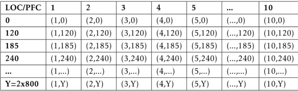
In this case, the best sample space representation of the problem is using a two-way table, as can be seen in figure3.1. This table was created by using two variables, PFC and LOC. So, it leads at 72 hypothesis that potentially can be the solution, it means, the less costly configuration, which includes the estimated losses cost.
Table 3.1: Two-way table that represents the sample space relatively the system configu-rations LOC/PFC 1 2 3 4 5 ... 10 0 (1,0) (2,0) (3,0) (4,0) (5,0) (...,0) (10,0) 120 (1,120) (2,120) (3,120) (4,120) (5,120) (...,120) (10,120) 185 (1,185) (2,185) (3,185) (4,185) (5,185) (...,185) (10,185) 240 (1,240) (2,240) (3,240) (4,240) (5,240) (...,240) (10,240) ... (1,...) (2,...) (3,...) (4,...) (5,...) (...,...) (10,...) Y=2x800 (1,Y) (2,Y) (3,Y) (4,Y) (5,Y) (...,Y) (10,Y)
It is pretended to achieve the minimum cost for the system by considering the config-uration that minimize the losses and at the same time, using the lowest possible initial investment cost. The investment considered in this dissertation is settled in the initial of
3 . 1 . M O D E L
times and includes the energy equipments that are inside the substations and the cable used as parallel feeder cable. To ensure the efficiency of operation, those equipments are sized in accordance to guarantee the trip conditions inserted, although, it is verified if there is overloads.
The equipments directly responsible to provide power for the line are the traction groups, which are composed by a traction transformer and a traction rectifier. so, they are chosen and sized take into account the operation consumption. In section3.1.1.1is detailed this process.
The figure3.10shows an example of a traction system power diagram. Those lines represents the power delivered by three substations, needed to ensure the operation, giving this way the energy the vehicle needs to perform properly, also includes the total losses
Figure 3.10: Example of consumption profile from three substations located consecutively in a track
The algorithm automatically incremented the traction groups, in substations, if needed, by incrementing the power capacity in equal values each time, in this case, 1000 kVA. So, consequently, it is quoted more traction groups to be added at the system’s cost.
In figure3.11 can be seen a substation single line diagram. As can be seen it is a basic representation of the components in a substation. The main energy equipments are considered in the quotation, in this dissertation, to estimate the overall substation cost. These components are: the traction group, composed by the traction transformer and rectifier, the medium voltage board, the low voltage system and the DC traction board.
3 . 1 . M O D E L
3.1.1.1 Sizing the power supply system
The simulation automatically sizes the substations and the cable section to use as parallel feeder cable. The scale of the substations is by comparing the nominal power of the traction transformer and rectifier with the power diagram curve. This comparison take into account in complying with the minimum electric requirements, mostly used by design systems, that is regarding the load/time duration.
To develop these process that is usually implemented by railway designers, the simu-lated configuration will be evaluated acceptable if the following conditions are verified.
• The maximum permanent current in contact wire is lower than the maximum con-sidered. If it was registered current overloads in contact line, it is increased the parallel feeder cable section, in order to decrease the resistance and solve the issue;
• The minimum contact line voltage is higher than 500V;
• The maximum permanent current delivered by substation is lower than 150% of the nominal value.
The figure 3.12 shows both the systems: the substations and the catenary system, which is composed by a contact wire and the positive parallel feeder cable.
Figure 3.12: DC traction system
The substations locations in the track are compliant with the following:
• TPS1 and TPS3 have pre-defined locations: in the beginning and in the end of the route, respectively;
• Resulted from simulation are the best location for the intermediate substation (TPS2). It is considered, by simplicity, nine possible locations (equally spaced along the track). In figure3.13can be seen a representation of these possible locations, the refereed percent values represents the distance relatively to the total length of the route.
Figure 3.13: Representation of possible TPS2 locations in percentage value of the total length of the route
The parallel feeder cable belongs to the distribution system, which is also composed by a fixed 120mm2section contact wire. In figure3.2can be seen the cables input database, to use as parallel feeder cable, during simulation.
Table 3.2: Parallel feeder cable used in the software tool
Code Id Section [mm2] Resistance [Ω/km] Maximum Capacity [A] PFC120 120 0.22 380 PFC185 185 0.148 420 PFC240 240 0.074 450 PFC400 400 0.044 821 PFC630 630 0.028 580 PFC800 800 0.022 620 PFC2x800 2x800 0.011 1238
3 . 1 . M O D E L
3.1.1.2 Investment cost in equipments
The estimation cost for traction equipment is based on the equipment’s unitary prices, that are predefined in the excel file. The values considered in this study are showed in table3.3and3.4.
Table 3.3: Substation Equipments considered and respective unitary prices
Substation Equipment Unit Cost [€/km] Traction Transformer 1000 kVA 30000
Rectifier 1000 kW 15000
Medium Voltage Board 50000
Low Voltage System 100000
Table 3.4: Considered cables and respective unitary prices
Cables Unit Cost [€/km]
PFC120 1400 PFC185 1900 PFC240 2800 PFC400 2950 PFC630 5200 PFC800 6400 PFC2x800 12300
Figure3.14is an inside overview from a substation with the considered equipments refereed in table3.3. The Low Voltage System represents the overall low voltage equip-ments, such as, the switchboards, the UPS, the control system, the voltage limit device and the auxiliary transformer. Those equipments aren’t the focus of this dissertation, the main intention in using them is to achieve a more estimated real cost for the substations.
Figure3.15is a representation of a typical electrification for a railway. The Parallel feeder cable, in this case the cable goes along the route by air, but it is common to see the cable going buried. Figure3.16shows a cross section of an insulated cable that is used as parallel feeder cable. In figure3.16can be seen a traction transformer.
Figure 3.14: Inside overview of a typical traction power substation [Adapted from Siemens]
3 . 1 . M O D E L
Figure 3.16: Cross section of a feeder underground cable
Figure 3.17: Example of a Traction Transformer, from Efacec Power Solutions Linkdin page.
3.1.2 Dynamic variables modelling
In this section can be seen the dynamic motion equations that models the system. The equation expressed in3.1is the Newton’s 2nd law and it is the fundamental equation.
Fin−Fext= m × a (3.1)
The acceleration is proportional to the resulting forces and it is dependent on the total mass of the vehicle. Finrelates the traction or braking effort required by the vehicle to
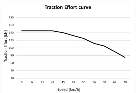
overcome the resistive forces Fext and operates. This parameter is introduced as a curve dependent on speed, as can be seen in figure3.18as example [13].
Figure 3.18: Typical traction and braking effort curves
In equation3.2can be seen all the drag forces used in the model. These forces are described in detail in sections3.1.2.1until3.1.2.2, [17].
Fext= Ff + Fa+ Fd+ Fc (3.2)
3.1.2.1 Motion Resistance
Running resistance
Running resistance is given by an empirical formula, as can be seen in equation3.3. This resistance depends on the vehicle weight, the mechanical frictions inside the vehicle, between wheels and rails and aerodynamic drags, [2] [22] [17].
Ff = A + BV + CV2 (3.3)
The coefficients A, B and C are constants and V is speed in m/s. These constant factors are obtained by fitting the coefficients of the Davis equation3.3. These coefficients are
3 . 1 . M O D E L
explained below.
The coefficient A is related to the drag between wheels and rails. Coefficient B comes from the quality of railway and the train stability. For this reason, they represent, the mechanical resistances of the vehicle with the railway. These terms have low relevance in low speed values.
At high speed, the term CV2, which is related to the aerodynamic resistance, becomes more relevant. This last term is largely affected by the existence of tunnels and the crossings with other vehicles, during the operation.
3.1.2.2 Declines Forces
During the passage trough an up climb, the gravity force applies a drag force to the train motion. In case of a down climb, this force favors the motion. This force is expressed by the equation3.4, [3], [17].
Fd= mgsen(α) (3.4)
Where, α > 0 in up climbs and α < 0 in down climbs.
3.1.3 Electrical system modelling
The modelling of the electrical system has been carried out by using the package sim-scape from Simulink. The electrical model is mainly composed by a source system, with three substations and an electrical distribution system, composed by variable resistances, that carry the energy to feed the load, that is the vehicle.
The power flow is modeled using dependent current sources and an additional logic blocks that controls them. This logic allows to ensure that there is just one vehicle running during the trip and that at each moment this current source receives the proper data. The source system has been developed by making use of a DC voltage source and a resistance in series. Figures3.19and3.20shows a detailed image of the electrical circuit blocks from simulink.
Figure 3.19: First electrical section circuit modelled in simulink
3 . 1 . M O D E L
The electrical power flow created by the vehicle has been simulated using the traction and braking force required and the speed that it goes, at each time. It was considered a yield value of 90%. So, the electrical power during traction and braking can be expressed by the equations3.5and3.6, respectively according the operation state, during traction or braking.
Pelect(t) =Fin(t) × v(t)
η (3.5)
Pelect(t) = Fin(t) × v(t) × η (3.6)
In figure3.12can be seen the representation of the traction system, including both systems: The supply system that is composed by three power substations, TPS1, TPS2 and TPS3. The distribution system is composed by the contact wire and the parallel feeder cable. Those two cables are shunted at middle way distance from substations, named feeder nodes.
The electric circuit is composed by two electrical sections, the first between TPS1 and TPS2 and the second between TPS2 and TPS3. Each one is mainly fed by two adjacent substations. Substations were designed using ideal 750Vdc voltage sources, each with 0.01 Ω/km internal resistance.
For example, when vehicle is moving between the beginning of the route and the shunt, the situation represented in3.21occurs. When the vehicle is operating after shunt, the resistances before shunt assumes constant resistance values.
Each feeder cable with different section is presented in the inputs file, as can be seen in table3.2.
Itrain(x) = Pelect(x) Vtrain(x)
(3.7)
3.1.3.1 Consumption and losses calculation
To ensure the operation, three substations are needed to provide sufficient energy. For this reason, consumption is calculated, as follows:
ET P S(t) = Z t t=0 Pelec(t) × ∆t 3600 [kW h] (3.8) where:
[∆t] - Sampling time considered, 1 second;
Pelec(t) - Substation power in each moment.
Figure3.22shows an example of substations power diagram curves.
Figure 3.22: Example of power diagram from three substations
The losses are calculated as follows:
Elosses= Ri·Ii2 =ρ · ` A ·I 2 i (3.9) where: ρ - Electrical resistivity [mΩ · m];
3 . 1 . M O D E L
` - length of the cable [m];
A - Cross Section of the cable [mm2];
Ii- Current in each branch of catenary system [A].
The estimated energy cost consumed during a life time depends on the energy used from substations. So, to evaluate each configuration, firstly is considered the power diagram curves from each substation. It was considered the operation works during 18 hours a day with an ideal headway, during weeks and weekends, for the considered life time. These approximation is acceptable because the intention is to calculate the consumption worst case scenario.
So the annual energy consumed is expressed by equation3.10.
ECON SU M= 3 X i=1 ET P Si· 60 HW ·18 · 365 [kW h] (3.10) where: P3
i=1ET P S - Sum of the energy consumption from traction power substations [kWh];
3.2
Financial evaluation
In this section is showed the financial evaluation of the model. This process aims to show the financial impact on the traction system configuration. All the energy is acquired from the same power source, even the energy that is wasted along the operation. So, these wastes are take into account in the total amount of the system cost.
The tariff considered to calculate the energy cost, is 0.1 €/kWh. This value is based on the values applied at Portugal industrial consumers, which is possible to see in table3.5. In the algorithm of this dissertation has been applied constant refresh rate of the energy price: 4%, in each year. This value has been chosen in order to be conservative.
Table 3.5: Tariff for sale to final customers in MV [Translated from ERSE, 2018b] MV long uses Tarrif
Active Energy (€/kWh) Description Prices
Peak hour 0,1382
Partial Peak hour 0,2201 Off Peak hour 0,0777
The equation used to calculate the final estimated minimum cost is showed in equation
3.11. This equation is the sum of the cost in equipments (substations and catenary) and the estimated consumption and losses costs.
cost = CostL+ CostP FC+ CostT P S+ CostCON SU M (3.11) where:
• CostL- Losses estimated cost;
• CostP FC - Parallel feeder cable investment cost;
• CostT P S - Substations equipments investment cost; • CostCON SU M - Consumption of the operation cost.
3 . 3 . G A M E T H O D
3.3
GA Method
In this section is presented an alternative method to find the optimal solution. This method applies genetic algorithm.
3.3.1 Genetic algorithm
The first step to apply the genetic algorithm is initiate the parameters for the function ga(). It is used to obtain the desire solution: the minimum cost for the traction system. Optimizing two variables: the distance between substations and the section for the paral-lel feeder cable.
Defining bounds for the variables in optimization allows the user to exclude some configurations from the simulation, for some reason. This way, the data sample is short-ened and possible cause a speed up on the simulation.
In table 3.6 is possible to see those bounds, in this case LOC1 and LOC12 is the location for substation TPS2 in the route and PFC1 and PFC2x800 is to the section for parallel feeder cable.
The last column, vector position, shows the vector that allows the algorithm, to get the respective input values of a configuration, in order to perform a simulation.
Table 3.6: Parameters bounds used in function @ga
Item Description Value [m] or [sq. mm] Respective Config Code Id Input parameters Vetor position LB Position TPS2 530 LOC1 1 LB Section feeder cable 120 PFC0 1 UB Position TPS2 4770 LOC9 9 UB Section feeder cable 1600 PFC2x800 8
The optimization has been carried out of the follow specifications:Generations, is the maximum number of generations considered for the algorithm and it is related to the size of the population, so, in this case, 5 generations shows to be enough to achieve the solution. The value of the population size has been 12.
The algorithm use three constraints, seen as follows. If one configuration doesn’t comply with the restrictions, the algorithm penalizes this solution, increasing the cost in very high values.
• VL> Vmin;
• IEQP FC< IEQP FC;
• IEQCW < IEQCW.
where:
• VL- Line voltage
• Vmin- Minimum line voltage, 500 V for 750V rated.
• IEQP FC - Equivalent Current in each feeder cable branch.
• IEQCW - Equivalent Current in each contact wire branch.
3.3.1.1 Cost Function
The cost function is, in fact, a performance finder, which tends to be a way to choose the best solutions, based in the value of this function. Equation3.12is a representation of the objective function, as can be seen, the estimated cost for parallel feeder cables, plus the cost considered for the wasted energy by catenary. Then is added the cost from the consumption and the investment in equipments for the substations.
cost = CostL+ CostP FC+ CostT P Ss+ CostCON SU M (3.12)
where,
• CostL- Losses from catenary: contact wire and parallel feeder cable; • CostP FC - Parallel feeder cable Investment;
• CostT P S - Traction Power Substations equipments Investment;
C
h
a
p
t
e
r
4
Ca s e S t u d y
In this chapter is presented the results from simulations and respective analysis. It is showed a comparative study between two case studies and it is evaluated and studied the relative best solution for the traction system. It was used the software tool described in the previous chapter to simulate the different configurations. Firstly, the considered inputs are showed and then can be seen the obtained results from simulation. After the respective analysis, it is shown the effect of the genetic algorithm to estimate the traction system cost, presenting the best cost-benefit solution.
4.1
Resume of the cases studies
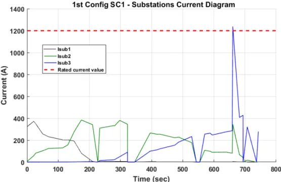
It is showed two case studies, named SC1 and SC2, each one includes a group of trac-tion system configuratrac-tions, aleatory chosen, in order to simulate and compare different scenarios regarding power supply. The main difference is the parallel feeder cable used and the intermediate substation location. The purpose of these comparative analysis is show the importance of optimizing and defining, conscientiously the traction system sup-ply configuration. So, it is showed the impact in use these configurations on the wasted energy by catenary. To conclude the analysis, it is showed an economical comparative result between the configurations.
To simulate those configurations, firstly, it is showed the considered input data and considerations, then are showed the outputs, such as, the speed and acceleration profiles, the vehicle position and vehicle consumptions along the route. As the vehicle operation is always in same conditions and assumptions, the load consumption is the same in all configurations, although changing the configuration will impact on the power supply behaviour. To study these impact electrical outputs are used and showed, such as, the
contact wire drop voltage and current values and substation consumptions.
The tool has been used to estimate the minimum cost involved in the system (the investment in feeder cable and the losses estimated cost from the catenary system). The variables considered to this study are, once more: the location for substation TPS2Loc and the section for parallel feeder cable PFC. It is pretended the algorithm finds the configuration [Loc;PFC] that leads to the minimum final cost.
4.1.1 Case Study input data
In this section is presented the inputs considered in the simulations for the case studies.
In table 4.1, is possible to see the speed limits profile in kilometers per hour in each position of the route and the respective resulted graph.
4 . 1 . R E S U M E O F T H E C A S E S S T U D I E S
Table 4.1: Input speed profile
Position [m] Speed Limits [km/h]
0 50 200 50 400 20 600 20 800 20 1000 60 1200 60 1400 30 1650 20 1700 20 1800 50 2000 50 2200 50 2350 20 2400 20 2600 20 3000 25 3500 40 3700 70 4000 70 4100 20 4300 20 4500 60 5100 20 5300 20
Table 4.2: Stations considered in simulation
Position [m] Station Name
0 Station 1 600 Station 2 1700 Station 3 2500 Station 4 4300 Station 5 5300 Station 6
In table4.3, can be seen the characteristics of the vehicle. It is recommended the user inserts the worst case data, regarding the consumption, that, in this case is considering the vehicle are fully loaded, so the weight corresponds to the vehicle tare plus its maximum capacity and the acceleration and deceleration values are the highest values that are allowed by the vehicle driver.
Table 4.3: Vehicle considered in simulation
Data Unit Value
Weight [kg] 123072 Constant Coefficient [N] 2199 Linear Coefficient [N] 50.4 Quadratic Coefficient [N] 4.53 Maximum Speed [km/h] 70 Maximum Acceleration [m/s2] 1.1 Maximum Deceleration [m/s2] 1.1 Minimum Voltage [Vdc] 500 Rated Voltage [Vdc] 750 Maximum Voltage [Vdc] 900 Auxiliary Loads [W] 106000 Maximum Traction Effort [N] 144840 Maximum Traction Current [A] 1587
The traction effort limitation curve can be seen in figure4.2. Table 4.4: Traction Effort
Speed [km/h] Traction Effort [N]
0 144840 6 144840 7 144840 25 144840 44 144840 45 140000 48 132200 50 125000 56 112000 60 105000 64 98000 70 90000
4 . 1 . R E S U M E O F T H E C A S E S S T U D I E S
Figure 4.2: Traction Effort limitation curve from the vehicle Table 4.5: Operation modes input data
Dwell time (seconds) 30
Headway (minutes) 15
Number of trains per hour 4 Number of Operations per day 64 Operation Time (h/day) 16 Number of Operations per year 26280 Operation Time (h/year) 5840
Regarding the operation, was inserted a headway of 15 minutes, which corresponds at four operations (trips) per hour. During a year the number of vehicles that ran on the route was 26280.
Since it is inserted the length of the operation route (d), in this case, 5.3 km, the algorithm calculates nine potential solutions regarding the substation TPS2 position to be located :TPS2 location. The values are presented in table4.6.
![Figure 2.6: Immediate energy exchange between trains by regenerative braking, from [29].](https://thumb-eu.123doks.com/thumbv2/123dok_br/19219938.962236/30.892.159.728.646.813/figure-immediate-energy-exchange-between-trains-regenerative-braking.webp)